Hadwiger Integration of Definable Functions

(1)

University of Pennsylvania

ScholarlyCommons

Publicly Accessible Penn Dissertations

Summer 8-12-2011

Hadwiger Integration of Definable Functions

Matthew Wright

University of Pennsylvania, mwright2@math.upenn.edu

Follow this and additional works at:http://repository.upenn.edu/edissertations

Part of theGeometry and Topology Commons

This paper is posted at ScholarlyCommons.http://repository.upenn.edu/edissertations/391

For more information, please contactlibraryrepository@pobox.upenn.edu. Recommended Citation

Wright, Matthew, "Hadwiger Integration of Definable Functions" (2011).Publicly Accessible Penn Dissertations. 391.

(2)

Hadwiger Integration of Definable Functions

Abstract

This thesis de nes and classi es valuations on de nable functionals. The intrinsic

volumes are valuations on "tame" subsets of R^n, and by easy extension, valuations on functionals on R^n with nitely many level sets, each a "tame" subset of R^n. We extend these valuations, which we call Hadwiger integrals, to de nable functionals on R^n, and present some important properties of the valuations. With the appropriate topologies on the set of de nable functionals, we obtain dual classi cation theorems for general valuations on such functionals. We also explore integral transforms, convergence results, and applications of the Hadwiger integrals.

Degree Type Dissertation

Degree Name

Doctor of Philosophy (PhD)

Graduate Group Mathematics

First Advisor Robert Ghrist

Keywords

hadwiger integration, intrinsic volume, integral geometry, topology, integration

(3)

HADWIGER INTEGRATION OF DEFINABLE FUNCTIONS

Matthew L. Wright

A Dissertation

in

Mathematics

Presented to the Faculties of the University of Pennsylvania in Partial

Fulfillment of the Requirements for the Degree of Doctor of Philosophy

2011

Robert Ghrist, Andrea Mitchell University Professor

Supervisor of Dissertation

Jonathan Block, Professor of Mathematics

Graduate Group Chairperson

Dissertation Committee

Robert Ghrist, Andrea Mitchell University Professor

(4)

Acknowledgments

I cannot possibly thank here everyone who has supported and encouraged me on the

long and difficult road that has lead to the completion of this thesis. Still, I would

be remiss not to acknowledge those who have been most influential.

I am deeply indebted to my thesis advisor, Robert Ghrist, for accepting me as his

first Penn Ph.D. student, taking me to applied topology conferences, encouraging me

when I was stuck on proofs, and teaching by example how to give excellent lectures.

Thanks to Yuliy Baryshnikov for his insight on valuations, suggesting the extension

of Hadwiger’s theorem, and serving on my thesis committee. I thank Robin Pemantle

for serving on the committees for my oral exam and my thesis. Thanks also to Michael

Robinson for the many conversations over the past two years, and for reviewing the

draft of this thesis.

I am grateful for many people at Penn who have made possible my years of study

here. Thanks to the graduate chairs Ching-Li Chi, Tony Pantev, and Jonathan Block,

for your faith that I would one day complete this degree. My graduate career would

(5)

much thanks to Janet Burns, Monica Pallanti, Paula Scarborough, and Robin Toney.

Thanks also to Jason DeVito for sharing an office with me for five years, and for

providing continual encouragement, conversation, and many memories.

Of course, I am most grateful for the support of my parents, Jack and Aleris

Wright, and my sister, Lenora Riley. Last but not least, thanks to the many math

teachers and professors who have taught me mathematics over the years. Special

thanks to Lamarr Widmer, Doug Phillippy, Patrick Lintner, and Anne Loso—you

(6)

ABSTRACT

HADWIGER INTEGRATION OF DEFINABLE FUNCTIONS

Matthew L. Wright

Robert Ghrist, Advisor

This thesis defines and classifies valuations on definable functionals. The intrinsic

volumes are valuations on “tame” subsets ofRn_{, and by easy extension, valuations on}

functionals onRn_{with finitely many level sets, each a “tame” subset of}_Rn_{. We extend}

these valuations, which we callHadwiger integrals, to definable functionals onRn_{, and}

present some important properties of the valuations. With the appropriate topologies

on the set of definable functionals, we obtain dual classification theorems for general

valuations on such functionals. We also explore integral transforms, convergence

(7)

List of Figures

2.1 Definition of intrinsic volumes . . . 8

2.2 Convergence of intrinsic volumes . . . 12

2.3 Projection of annulus . . . 14

3.1 Flat norm illustration . . . 22

3.2 Normal cycle of a simplicial complex . . . 24

3.3 Conormal cycle of an interval . . . 27

4.1 Hadwiger integral definition . . . 34

4.2 Hadwiger integral by level sets and slices . . . 35

4.3 Example function . . . 40

5.1 Different topologies . . . 52

5.2 Decreasing composition . . . 56

5.3 Excursion sets . . . 61

6.1 -tube example . . . 64

(11)

6.3 Non-convex convolution example . . . 66

6.4 Reach of a set . . . 67

6.5 Definable convolution example . . . 71

7.1 Nonconvergence example . . . 77

7.2 Circle packing . . . 80

8.1 Cell structure . . . 94

(12)

Chapter 1 Introduction

How can we assign the notion of “size” to a functional—that is, a real-valued function—

on Rn_{? Surely the Riemann-Lebesgue integral is one way to quantify the size of a}

functional. Yet are there other ways? The integral with respect to Euler

character-istic gives a very different idea of the size of a functional, in terms of its values at

critical points. Between Lebesgue measure and Euler characteristic lie many other

pseudo-measures (or more properly, valuations) known as theintrinsic volumes, that

provide notions of the size of sets in Rn_{. Integrals with respect to these intrinsic}

volumes integrals provide corresponding quantifications of the size of a functional.

In this thesis, we explore the integration of continuous functionals with respect

to the intrinsic volumes. The approach is o-minimal and integral. First, in order to

develop results for “tame” objects, while excluding pathologies such as Cantor sets

(13)

in terms of an o-minimal structure. The particular o-minimal structure is not so

important, though for concreteness the reader can think of it as being comprised of

all subanalytic sets, or all semialgebraic sets. Use of an o-minimal structure makes

the discussion context-free and applicable in a wide variety of situations. Second, the

approach isintegral in the sense that we are not primarily concerned with valuations

of sets, but instead with integrals of functionals over sets. Valuations of sets have

been well-studied in the past; much less is known about valuations of functionals.

The setting of this work is in applied topology and integral geometry. Indeed, the

motivation for this research is to answer questions that arise in sensor networks, a key

area of applied topology. Integral geometry is an underdeveloped, intriguing subject

that studies symmetry-invariant integrals associated with geometric objects [6, 21].

The study of such integrals involves important techniques from geometric measure

theory, especially the theory of currents. Furthermore, the work has important

con-nections to combinatorics: the intrinsic volumes can be studied from a combinatorial

perspective, as presented by Klain and Rota [24], and involving a triangular array of

numbers known as the flag coefficients.

Chapter 2 contains an o-minimal approach to the intrinsic volumes. Beginning

with Hadwiger’s formula, we establish various equivalent expressions of the intrinsic

volumes, all applicable in the o-minimal setting. Perhaps the most intriguing and

least-known expression has to do with currents, which we explain in Chapter 3.

(14)

important properties of integrals with respect to intrinsic volumes. We call such

an integral a Hadwiger integral. Hadwiger integrals can be expressed in various

ways, corresponding with the different expressions of the intrinsic volumes. We

en-counter a duality of “lower” and “upper” integrals, which are not equivalent, but

arise due to the differences in approximating a continuous function by lower- and

upper-semicontinuous step functions.

Next, we discuss general valuations on functionals, and classify them in Chapter

5. The duality observed earlier is again present, with “lower” and “upper” valuations

that are continuous in different topologies. This leads to our main result:

Main Theorem. Any lower valuationv onDef(Rn₎_{can be written as a linear}

com-bination of lower Hadwiger integrals. For h∈Def(Rn₎_,

v(h) =

n

X

k=0

Z

Rn

ck(h) bdµkc,

where the ck :R→R are increasing functions with ck(0) = 0.

Likewise, an upper valuation v on Def(Rn₎_{can be written as a linear combination}

of upper Hadwiger integrals.

Chapter 6 explores integral transforms, which are important in applications. In

particular, we examine convolution, where the convolution integral is with respect to

the intrinsic volumes. We also consider integral transforms analogous to the Fourier

and Bessel (or Hankel) transforms.

(15)

is important in applications. Thus, Chapter 7 provides further results related to

estimation and convergence of Hadwiger integrals.

Chapter 8 discusses known and speculative applications of this valuation theory, as

well as opportunities for future research. Applications include sensor networks, image

processing, and crystal growth and foam dynamics. In order that Hadwiger integrals

may be more easily applied, we need further research into index theory, algorithms,

and numerical analysis of the integrals. We could also study more general valuations,

(16)

Chapter 2 Intrinsic Volumes

The intrinsic volumes are the n + 1 Euclidean-invariant valuations on subsets of

Rn_{. This chapter provides the background information necessary to understand the}

intrinsic volumes in an o-minimal setting.

2.1 Valuations

A valuation on a collection of subsets _S of Rn _{is a function} _v _:_{S →} _R _{that satisfies}

the additive property:

v(A∪B) +v(A∩B) =v(A) +v(B) for A, B ∈ S.

On “tame” subsets of Rn _{there exist} _n _{+ 1 Euclidean-invariant valuations. These}

often appear in literature by the names intrinsic volumes and quermassintegrale,

(17)

Hadwiger measures, Lipschitz-Killing curvatures, and Minkowski functionals. Here

we will primarily refer to these valuations as intrinsic volumes to emphasize that

the intrinsic volumes of A _{∈ S} are intrinsic to A and do not depend on any

higher-dimensional space into whichA may be embedded.

The literature defines the intrinsic volumes in various ways. Klain and Rota [24]

take a combinatorial approach, defining the intrinsic volumes first on parallelotopes

via symmetric polynomials, then extending the theory to compact convex sets and

finite unions of such sets. Schneider and Weil [41] define the intrinsic volumes and

quermassintegrale on convex bodies as coefficients of the Steiner formula, which we

will discuss in Section 6.1. Morvan [32] takes a similar approach via the Steiner

for-mula. Santal´o [35] approaches the quermassintegrale as an average of cross-sectional

measures. Schanuel [38] and Schr¨oder [42] provide short, accessible introductory

pa-pers on the intrinsic volumes.

We will define the intrinsic volumes in a way lends itself to the integration theory

that is our goal. Thus, instead of working with sets that are compact or convex, we

will begin with an o-minimal structure that specifies “tame” subsets of Rn_{. Van den}

Dries [43] defines an o-minimal structure as follows:

Definition 2.1. An o-minimal structure is a sequence _S = (_Sn)n∈N such that:

1. for each n, _Sn is a boolean algebra of subsets of Rn—that is, a collection of

subsets of Rn_{, with} _{∅ ∈ S}

n, and the collection is closed under unions and

(18)

2. _S is closed under projections: if A _{∈ S}n, then π(A) ∈ Sn−1, where π : Rn →

Rn−1 _{is the usual projection map;}

3. _S is closed under products: if A_{∈ S}n, then A×R∈ Sn+1;

4. _Sn contains diagonal elements: {(x1, . . . , xn) ∈ Rn | xi = xj for 1 ≤ i < j ≤

n} ∈ Sn;

5. S1 consists exactly of finite unions of points and (open, perhaps unbounded)

intervals.

Examples of o-minimal structures include the semilinear sets, the semialgebraic

sets, and many other interesting structures. The definition of an o-minimal structure

S prevents infinitely complicated sets such as Cantor sets from being included in _S.

Elements ofSn we calldefinable sets. A mapf :Rn→Rm whose graph is a definable

subset ofRn+m _{is a}_{definable map}_{. To explain the name}_o-minimal_{, the “o” stands for}

order, and “minimal” refers to axiom 5 of Definition 2.1, which establishes a minimal

collection of subsets of R.

The o-minimal Euler characteristic, denoted χ, is defined so that for any open k

-simplexσ,χ(σ) = (₋1)k_{, and to satisfy the additive property. Since any definable set}

is definably homeomorphic to a disjoint union of open simplices, Euler characteristic is

defined onS. The o-minimal Euler characteristic coincides with the usual topological

Euler characteristic on compact sets, but not in general. In particular, the usual

(19)

K

P4

P1 P2

P3

P5

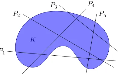
Figure 2.1: The intrinsic volumeµk of subsetK ⊂Rn is defined as the integral over

all affine (n−k)-planes P of the Euler characteristic χ(K∩P), as in Definition 2.2.

that which arises from the Borel-Moore homology, but it is not a homotopy invariant.

2.2 Definition via Hadwiger’s formula

In this paper,Gn,k denotes the Grassmanian ofk-dimensional linear subspaces ofRn,

and An,k denotes the affine Grassmanian of k-dimensional affine subspaces of Rn.

Definition 2.2. For a definable set K ∈ Sn, and k = 0,1, . . . , n, define the kth

intrinsic volume, µk, of K as

µk(K) =

Z

An,n−k

χ(K_∩P) dλ(P) (2.1)

where λ is the measure onAn,n−k described below.

Equation (2.1) is known as Hadwiger’s formula. Figure 2.1 illustrates the

defini-tion of the intrinsic volumes in terms of integrals over affine planes.

(20)

Gn,n−k. That is, P is uniquely determined byLand a vectorx∈Rk,x⊥P, such that

P = L+x. Thus, we can integrate over An,n−k by first integrating over Gn,n−k and

then over Rk_{. Equation (2.1) is equivalent to}

µk(K) =

Z

Gn,n−k

Z

Rk₍_L₎

χ(K_∩(L+x)) dx dγ(L) (2.2)

where L ∈ Gn,n−k, x ∈ Rk is orthogonal to L. Let γ be the Haar measure on the

Grassmanian, scaled so that

γ(Gn,m) =

n m

ωn

ωmωn−m

(2.3)

with ωn denoting the n-dimensional volume of the unit ball in Rn. We can express

ωn in terms of the Gamma function:

ωn=

πn/2 Γ(n/2 + 1).

We scale the measure of the Grassmanian to satisfy equation (2.3) because this

makes the intrinsic volume of a set K independent of the dimension of the space

in which K is embedded. For example, if K is a 2-dimensional set in R3 _(so _K _is

contained in a 2-dimensional plane), thenµ2(K) is the area of K. The valuations µk

areintrinsic in the sense that they depend only on the sets on which they are defined,

and not on the dimension of the ambient space.

Observe that µ0 is Euler characteristic and µn is Lebesgue measure onRn:

µ0(K) =

Z

1

χ(K∩Rn₎ _dλ₌_χ₍_K₎ _and _µ

n(K) =

Z

Rn

(21)

The kth _{intrinsic volume,} _µ

k, provides a notion of thek-dimensional size of a set. For

example,µ1 gives an idea of the “length” of a set, as Schanuel describes in his classic

paper, “What is the length of a potato?” [38].

It follows from equation (2.2) that the intrinsic volumeµkishomogeneous of degree

k. That is, µk(aK) = akµk(K), for all a ≥ 0 and definable K. Also note that any

intrinsic volume of the empty set is zero. By definition, χ(_∅) = 0, and equation (2.1)

implies that also µk(∅) = 0.

The numbers _mn _ω_n

ωmωn−m in equation (2.3) are called flag coefficients and are

analogous to the binomial coefficients [24]. As the binomial coefficient n_k

counts

the number of k-element subsets of an n-element set, the flag coefficient _mn _ω_n

ωmωn−m

gives the measure ofk-dimensional linear subspaces ofRn_{. That is, we scale the Haar}

measure on the grassmanian Gn,m so that equation (2.3) holds. This is precisely the

scaling necessary to make the intrinsic volumes intrinsic. For more about the flag

coefficients, see Appendix A.

The quermassintegrale differs from the intrinsic volumes only in terms of

normal-ization. For definableK _⊂Rn_{and integer 0} _≤_k _≤_n_{, the quermassintegrale}_W n,k(K)

is defined

Wn,k(K) =ωk

n k

−1

µn−k(K). (2.4)

Unlike the intrinsic volumes, the quermassintegrale depends on the dimension of the

(22)

2.3 Important Properties

The intrinsic volumes enjoy the important properties of additivity and Euclidean

invariance, as in the following proposition.

Proposition 2.1. For definable sets A, B _⊂ Rn_{, and} _k _{= 0}_,₁_{, . . . , n}_{, the following}

properties hold:

• Additivity: µk(A∪B) +µk(A∩B) =µk(A) +µk(B).

• Euclidean invariance: µk(A) = µk(φ(A)) for φ ∈ On, the group of orthogonal

transformations on Rn.

Proof. Additivity follows from the fact that Euler characteristic is additive:

χ(A∪B) +χ(A∩B) =χ(A) +χ(B).

Euclidean invariance follows from the fact that the integral over the affine

Grass-manian is invariant under rigid motions of Rn_.

Indeed, additivity is the key property that allows us to call µk a valuation. By

induction, the intrinsic volumes satisfy the inclusion-exclusion principle,

µk(K1∪ · · · ∪Km) = m

X

r=1

(−1)r−1 X

1≤i1<···<ir≤m

µk(Ki1 ∩ · · · ∩Kir)

for K1, . . . , Km ∈ S.

The intrinsic volumes are continuous in the sense that if J and K are convex

(23)

K1 K2 K3 K4 K5 K6

· · ·

K_∞

Figure 2.2: The intrinsic volumes of the Kn converge to those of K∞.

the Hausdorff distance between J and K is the smallest such that no point in J is

farther than from some point in K, and vice-versa. Formally, Hausdorff distance

between J and K can be written

dH(J, K) = max{sup x∈J

inf

y∈Kd(x, y),sup_y_∈_Kxinf∈Jd(x, y)}.

As an example of continuity, let _{Kj} be a sequence of n-dimensional sets that

converge in the Hausdorff metric to an (n−1)-dimensional setK∞, as illustrated in

Figure 2.2. Then,

lim

j→∞µk(Kj) =µk(K∞).

This is one justification why µn−1(K) is equal to half the surface area of K.

The intrinsic volumes are not continuous for definable sets in general with respect

to the Hausdorff metric. For example, a bounded convex set can be approximated

arbitrarily closely in the Hausdorff metric by a large discrete set. However, a compact

convex set has Euler characteristic one, while the Euler characteristic of a discrete

set equals its cardinality.

The intrinsic volumes are continuous on definable sets with respect to a topology

(24)

It is a well-known theorem of Hugo Hadwiger [23] that any continuous valuation

on convex subsets of Rn _{is a linear combination of the intrinsic volumes:}

Hadwiger’s Theorem. If v is a Euclidean-invariant, additive functional on subsets

of Rn, continuous on convex subsets with respect to the Hausdorff metric, then

v =

n

X

k=0 ckµk

for some real constantsc0, . . . , cn. Furthermore, if v is homogeneous of degreek, then

v =ckµk.

We will not reproduce the proof of Hadwiger’s Theorem here, but it may be found

in a variety of sources [12, 24, 41].

Definition 2.2 allows us to express the intrinsic volumesµk(K) in terms of “slices”

of K along affine (n₋k)-dimensional planes. Recall equation (2.1),

µk(K) =

Z

An,n−k

χ(K_∩P)dλ(P).

We can also expressµk(K) in terms of projections ofK ontok-dimensional planes.

Instead of integrating χ(K_∩P) for all affine (n₋k)-planes P, we can change our

perspective and project K onto linear k-subspaces L. In particular, let πL : K → L

be the projection map ontoL_∈Gn,k. For any x∈L, π−L1(x) is the fiber over x, that

is, the set of all points in K that are projected to x. We then have:

µk(K) =

Z

An,n−k

χ(K_∩(P))dλ(P) =

Z

Gn,k

Z

L

χ(π−_L1(x))dx dγ(L).

(25)

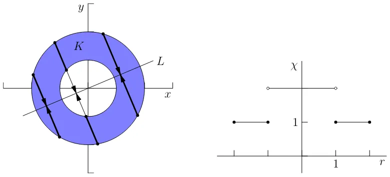
y

x K

L _χ

r 1

1

Figure 2.3: At left, the annulusK ⊂R2 _{is projected orthogonally onto an arbitrary}

linear subspace L _∈ G2,1. At right, the graph of χ(πL−1(r)), the Euler characteristic

of the fibers of the projection of K onto L.

Theorem 2.1 (Projection Formula). For any definable set K in Rn and 0≤k ≤n,

µk(K) =

Z

Gn,k

Z

L

χ(π_L−1(x)) dxdγ(L)

where π−_L1(x) is the fiber over x_∈L of the orthogonal projection map πL:K →L.

Example. Consider the annulusK _⊂R2 _{in Figure 2.3, with inner radius 1 and outer}

radius 2. We compute µ1(K) via the projection formula.

Let L _∈ G2,1 be an arbitrary line through the origin. Several fibers of the

pro-jection map πL onto L are indicated at left in Figure 2.3. The Euler characteristic

χ(π−_L1(r)) is graphed at right in Figure 2.3 as a function of r, the position along L,

measured from the origin. By rotational symmetry about the origin,χ(π−_L1(r)) is the

(26)

Integrating, we find that R

Lχ(π−

1

L (r)) dr= 6. Then,

µ1(K) =

Z

G2,1

Z

L

χ(π−_L1(r))dr dγ(L) =

Z

G2,1

6dr = 6· π

2 = 3π. (2.5)

This computation agrees with the previous assertion thatµn−1 equals half the surface

area of an n-dimensional set. Here, µ1(K) = 3π, which is half the (combined inner

and outer) perimeter of the annulus.

The situation is simpler if K is compact and convex: In this case, χ(π−_L1(x)) = 1

for all L ∈ Gn,l and x ∈ L. Thus, the projection formula, Theorem 2.1, reduces to

the standard mean projection formula [24]:

Theorem 2.2(Mean Projection Formula). For0_≤k _≤n and compact convex subset

K of Rn,

µk(K) =

Z

Gn,k

µk(K|L) dγ(L)

where the integrand is the k-dimensional volume of the projection of K onto a k

-dimensional subspace L of Rn.

Proof. For any P ∈Gn,n−k, the intersectionK∩P is also compact convex, so χ(K∩

P) = 1. Accordingly, for L _∈ Gn,k, every nonempty fiber π−L1(x) is also compact

convex, so χ(π−_L1(x)) = 1. Thus, R

Lχ(π−

1

L (x)) dx is the k-dimensional (Lebesgue)

volume of the projection of K onto L. Let K|L denote the projection of K onto L.

Then,

µk(K) =

Z

Gn,k

Z

L

χ(π_L−1(x)) dx dγ(L) =

Z

Gn,k

(27)

The mean projection formula gives another justification of why µn−1(K) is half

the surface area of K ⊂ Rn_{. First, let} _K _{be a convex polyhedron in} _Rn_{. For each}

face fi of K, µn−1(fi|L) is the area of the projection of fi onto L ∈ Gn,k. Since the

projection map ofK ontoL covers each point in its image twice, we have

X

i

µn−1(fi|L) = 2µn−1(K|L).

Integrating over the GrassmanianGn,n−1 and applying the Mean Projection Formula,

we obtain

X

i

µn−1(fi) =

Z

Gn,n−1

X

i

µn−1(fi|L) dγ(L)

=

Z

Gn,n−1

2µn−1(K|L) dγ(L) = 2µn−1(K). (2.6)

Now P

iµn−1(fi) is the surface area of K, so equation (2.6) implies that the surface

area of K is 2µn−1(K). Since any convex subset is a limit of convex polyhedra, the

result holds for all convex subsets of Rn_{. By additivity, it holds for definable subsets}

of Rn_.

We can express an intrinsic volume of a direct product in terms of the intrinsic

volumes of its factors:

Theorem 2.3 (Product Theorem). For J, K _{∈ S},

µk(K×J) = k

X

i=0

µi(K)µk−i(J). (2.7)

Klain and Rota prove the Product Theorem using Hadwiger’s Theorem [24].

(28)

[41]. Representing the intrinsic volumes in terms of conormal cycles, we exhibit a

more elegant proof of the Product Theorem, as we will discuss in Section 3.4.

One implication of the Product Theorem is that µk(K ×J) can be computed by

integrating over only those affine (n₋k)-planes that are themselves direct products of

affine planes in the factor subspaces containing K and J. Furthermore, the Product

Theorem extends to direct products of many definable sets:

Corollary 2.1. For K1, . . . , Kr ∈ S,

µk(K1× · · · ×Kr) =

X

i1+···+ir=k

µi1(K1)· · ·µir(Kr). (2.8)

Proof. Identity (2.8) follows by induction from Theorem 2.3.

2.4 Intrinsic Volumes of Common Subsets

We can now compute the intrinsic volumes of closed balls and rectangular prisms.

Example. Let Bn be the closed n-dimensional unit ball, and ωn its volume. We will

compute µk(Bn):

µk(Bn) =

Z

Gn,n−k

Z

Rk₍_L₎

χ(Bn∩(L+x))dxdγ(L)

=

Z

Gn,n−k

Z

Bk

1dxdγ(L)

=

Z

Gn,n−k

ωk dγ(L) =

n k

ωn

ωn−k

.

Example. LetK be a closedn-dimensional rectangular prism in Rn _{with side lengths}

(29)

follows:

µk(K) =µk([0, x1]× · · · ×[0, xn])

= X

i1+···+in=k

µi1([0, x1])· · ·µir([0, xn])

= X

i1+···+in=k

xi1

1 · · ·xinn wherei1, . . . , in∈ {0,1}

= X

1≤j1<···<jk≤n

xj1· · ·xjk

and this is the elementary symmetric polynomial of degree k on the n variables

x1, . . . , xn.

2.5 Open Sets

Our o-minimal approach to the intrinsic volumes prompts us to consider the intrinsic

volumes of non-compact sets, and in particular, open sets. Indeed, in applications we

will need to be able to compute the intrinsic volumes for open sets. To begin, recall

that if σ is an openk-dimensional simplex, thenχ(σ) = (−1)k_.

A regular open set is equal to the interior of its closure, and a regular closed set

is equal to the closure of its interior. That is, K is regular open if K = Int(K), and

J is regular closed if J = IntJ.

We have the following lemma:

Lemma 2.1. Let K be a definable, regular closed set in Rd. Then χ(IntK) =

(30)

We defer the proof of Lemma 2.1 until Section 4.2.

The lemma leads to a similar result for the intrinsic volumes:

Theorem 2.4. LetK be definable in Rn, such thatK = IntK andK is not contained

in any (n₋1)-dimensional affine subspace of Rn. Then,

µk(IntK) = (−1)n+kµk(K).

Proof. For any P ∈An,n−k, K∩P is a subset, equal to the closure of its interior, of

dimension n₋k. Note that Int(K_∩P) = (IntK)_∩P, so by the lemma we have:

χ(Int(K _∩P)) = (₋1)n−k_χ₍_K_∩_P₎_.

Integrating over An,n−k, we obtain:

µk(IntK) =

Z

An,n−k

χ((IntK)_∩P) dλ(P)

= (−1)n−kχ(K∩P) dλ(P) = (−1)n−kµk(K).

While the Lebesgue measure of a definable set and its closure are the same, the

intrinsic volumes are, in general, very sensitive to boundary points. When computing

the intrinsic volumes of a set, it is essential to note whether the set contains some or all

of its boundary. An understanding of this detail will be important to the integration

(31)

Chapter 3 Currents and Cycles

The intrinsic volumes also arise from integration of differential forms over normal and

conormal cycles of sets. Normal and conormal cycles are examples ofcurrents, which

are continuous linear functionals on the spaces of differential forms. This chapter

gives a brief introduction to currents, providing only information relevant to our

applications. For more details, see chapter 7 of Krantz and Parks [25], chapter 12 of

Morvan [32], or the exhaustive and technical chapter 4 of Federer [16].

3.1 Currents

First we must establish some notation. Let Ωk

c(U) denote the space of

compactly-supported differential k-forms on some U _⊆ RN_{. Its dual space, the space of}

con-tinuous linear functionals on Ωk

c(U), we denote as Ωk(U), or simply as Ωk if U is

(32)

bound-ary of a currentT _∈Ωk is the current∂T ∈Ωk−1 defined by (∂T)(ω) = T(dω) for all

ω ∈ Ωk−1

c . A cycle is a current with zero boundary. Similarly to differential forms,

∂(∂T) = 0.

Currents are naturally associated with submanifolds and geometric subsets [25,

32]. Let Mn _{be a} _C1 _oriented _n_{-dimensional submanifold of} _RN_{. Let} _dv

Mn be the

volume form on Mn_{. For any} _ω_∈_Ωk

c(RN), the restriction of ω toMn equals fωdvMn

for some function fω on Mn. Define a current [[Mn]] associated toMn by

[[Mn]](ω) =

Z

Mn

fωdvMn.

For our work with currents, we need a norm on the space of currents. First, the

mass M(T) of a current T _∈Ωk(U) is the real number defined by:

M(T) = sup{T(ω)| ω ∈Ωkc(U) and sup|ω(x)| ≤1 ∀x∈U}.

The mass of a current generalizes the volume of a submanifold: the mass of a current

supported on a tame set is equal to the volume of the set. Second, let_|T_|_[ denote the

flat norm of the current T _∈Ωk(U), which is the real number defined by:

|T|[ = inf{M(R) +M(S)| T =R+∂S, R∈Ωk(U), S∈Ωk+1(U)}. (3.1)

We can think of the flat norm as quantifying the minimal-mass decomposition of a

k-currentT into ak-currentR and the boundary of a (k+ 1)-currentS, as illustrated

in Figure 3.1. The flat norm is an excellent tool for measuring the distance between

(33)

T =R+∂S ∈Ω1 R∈Ω1 S ∈Ω2

Figure 3.1: The 1-current T is decomposed as the sum of a 1-current R and the

boundary of a 2-current S. Intuitively, the flat norm of T is the decomposition that

minimizes the length of R plus the area of S.

In this context, the word “flat” is not referring to a lack of curvature, but simply to

Hassler Whitney’s musical notation[ used to denote this norm [25, 30].

3.2 Normal and Conormal Cycles

We are interested in particular currents, known as the normal cycle and conormal

cycle, that are associated to compact definable sets. The normal cycle is a

general-ization of the unit normal bundle of a manifold. The definition of the normal cycle is

long and technical; for that we refer the reader to Bernig [7], Fu [20], or Nicolaescu

[34]. Let A be a compact definable set in RN_{. We denote the normal cycle of} _A _as

NA_{. Formally,} _NA _{is an (}_N ₋_{1)-current on the unit cotangent bundle} _RN _×_SN−1_.

(34)

1-form α on the tangent bundle T∗_RN _{is zero:}

NA

α = 0.

The key property for our purposes is that the normal cycle is additive, that is:

NA∪B+NA∩B =NA+NB. (3.2)

Intuitively, we regard NA _{as the collection of unit tangent vectors to} _A_{, though}

this intuition is inadequate ifAis not convex. More precisely, ifAis a convex set, then

the support of NA _{is the hypersurface of unit tangent vectors to} _A_{, with orientation}

given by the outward normal.

Example (Normal cycle of a simplicial complex). If σ is a (closed) k-simplex in RN_,

thenNσ _{is the current whose support is the surface of unit tangent vectors to}_σ_{, with}

outward orientation. We can then construct the normal cycle of a simplicial complex

via equation (3.2).

Figure 3.2 illustrates the normal cycle of a simplicial complex. The simplicial

complex K in R2 _{consists of the union of the two closed intervals} _ab _and _bc_{. The}

normal cycle of a closed interval in R2 _{is supported on an oriented path at unit}

distance around the interval. The intervals intersect at point b, whose normal cycle

is supported on an oriented unit circle at b. By equation (3.2),

NK =Nab+Nbc₋Nb,

(35)

a

b c

Figure 3.2: Normal cycle of a simplicial complex.

Dual to normal cycles are conormal cycles. For details on the construction of the

conormal cycle, see Nicolaescu [33]. The conormal cycle ofA, denoted CA_{, is also an}

(N −1)-current on RN _×_SN−1_{, and it is the cone over} _NA_{. The conormal cycle is}

Lagrangian, which means that its restriction to the standard symplectic 2-formω on

T∗_RN _{is zero:}

CA

ω = 0.

For example, the conormal cycle of an interval [a, b] inRis illustrated by the dark

path in Figure 3.3.

Pioneers in the study of normal and conormal cycles were Wintgen [46] and Z¨ahle

[47]. Fu gives a detailed treatment of these cycles of subanalytic sets in [19].

Nico-laescu shows in [33] the existence and uniqueness of normal and conormal cycles for

(36)

3.3 Lipschitz-Killing Curvature Forms

The intrinsic volumes arise from integrating certain differential forms over normal and

conormal cycles. These differential forms are called the Lipschitz-Killing curvature

forms, named after Rudolf Lipschitz and Wilhelm Killing. These forms are invariant

under rigid motions, as they must be since the intrinsic volumes are invariant under

such motions.

Since normal and conormal cycles are (N ₋1)-currents on RN _×_SN−1_{, we need}

differential (N₋1)-forms onRN_×_SN−1 _{invariant under rigid motions. Let}_x

1, . . . , xN

be the standard orthonormal basis for RN_{, and} _ρ

1, . . . , ρN−1 an orthonormal frame

for SN−1_{. Define the following differential (}_N ₋_{1)-form on} _RN _×_SN−1_:

V(t) = (x1+tρ1)∧ · · · ∧(xN−1+tρN−1).

Intuitively, if t = 0, this is the volume form on RN−1_{, which is invariant under rigid}

motions. Morvan explains in [32, ch. 19] that the form _V(t) is invariant under rigid

motions ofRN_{, extended to} _RN _×_SN−1_{, for all} _t_{. Fu arrives at the same result via a}

pushforward of an exponential map [21].

We can view the differential form_V(t) as a polynomial int, whose coefficients are

the invariant forms that we seek:

Definition 3.1. For 0_≤k _≤N ₋1, let _WN−1,k be the coefficient of tN−k−1 in V(t).

The form WN−1,k is called the kth Lipschitz-Killing curvature form of degree N −1.

(37)

multiples) over normal or conormal cycles of sets to obtain the intrinsic volumes. By

invariance, they do not depend on the orthonormal frame x1, . . . , xN, ρ1, . . . , ρN−1.

Indeed, Morvan states that the vector space of invariant differential (N₋1)-forms on

RN _×_SN−1 _{is spanned by the} _W

N−1,k and, if N is odd, by a power of the standard

symplectic form. However, the conormal cycle vanishes on the standard symplectic

form, so the only invariant forms relevant to our discussion are the_WN−1,k.

3.4 Back to the Intrinsic Volumes

We can express the intrinsic volumes in terms of normal or conormal cycles, and the

Lipschitz-Killing curvature forms.

Theorem 3.1. Let K ∈Def(Rn₎_{. The integrals}

Z

NKWn,k

and

Z

CK Wn,k

(3.3)

are, up to a constant multiple, the intrinsic volume µk(K).

Proof. Since the normal and conormal cycles are additive, and the Lipschitz-Killing

curvature forms are Euclidean-invariant, the integrals in (3.3) are valuations on

Def(Rn_{). By definition of the Lipschitz-Killing curvature forms, these expressions}

are homogeneous of degree k. The integrals are also continuous on convex sets with

respect to the Hausdorff metric. Therefore, by Hadwiger’s Theorem, these integrals

(38)

ρ

x a

b η

Figure 3.3: Conormal cycle of the interval [a, b].

Some low-dimensional examples will help illustrate this “current” approach to the

intrinsic volumes.

Example. Consider the interval [a, b]_⊂R. Its conormal cycleC[a,b]_{can be represented}

by the dark path in Figure 3.3. The space of invariant 1-forms on R2_×_S1 _{is spanned}

by the two forms W1,0 =dρ and W1,1 =dx. We obtain the intrinsic volumes of [a, b]

by the integrals:

µ0([a, b]) =

Z

C[a,b]

1

2π dρ= 1

µ1([a, b]) =

Z

C[a,b]

dx=b−a.

(39)

contains the following forms:

W2,0 =dρ1∧dρ2

W2,1 =dρ1∧dx2+dx1∧dρ2

W2,2 =dx1∧dx2

We obtain the intrinsic volumes ofK by integrating these forms over CK_:

µ0(K) =

Z Z

CK

1

4π dρ1∧dρ2

µ1(K) =

Z Z

CK

1

2π dρ1∧dx2+ 1

2π dx1∧dρ2

µ2(K) =

Z Z

CK

dx1∧dx2.

In the above examples, we use normalizations such as 1

2π to scale the integrals

properly, as is necessary for computations.

Representing the intrinsic volumes in terms of integrals of the Lipschitz-Killing

curvature forms, we can now prove the Product Theorem (Theorem 2.3). The key

observation is that by Definition 3.1, for integers 0< m < n,

Wn,k = k

X

i=0

Wm,i∧ Wn−m,k−i.

Therefore,

k

X

i=0

µk(K)µk−i(J) = k

X

i=0

Z

CKW m,i

Z

CJW

n−m,k−i =

Z

CK×JW

n,k =µk(K×J)

(40)

3.5 Continuity

The flat norm on conormal cycles is the key ingredient of a topology on definable

sets, with respect to which the intrinsic volumes are continuous.

Let A and B be definable subsets of Rn_{. Define the} _{flat metric} _{in terms of the}

flat norm as follows:

d(A, B) =CA−CB

[. (3.4)

Call the topology on definable subsets of Rn _{induced by the flat metric the} _flat

topology. The flat topology is a useful generalization of the Hausdorff topology on

convex sets. Indeed, if a sequence of convex sets converges in the Hausdorff topology,

then the corresponding sequence of their normal cycles converges in the flat topology

[17], but the same is not true for non-convex sets. On the other hand, convergence of

normal cycles of definable sets implies convergence in the Hausdorff topology.

Fur-thermore, we have the following theorem:

Theorem 3.2. The intrinsic volumes are continuous with respect to the flat topology.

Proof. LetK _∈Def(Rn_{) be bounded and}_>_{0. Let}_B _{be a large ball in}_Rn_containing

a neighborhood of K.

From the definition of flat norm, we have for any T _∈ Ωn and ω ∈ Ωnc, both

supported on B:

|T(ω)| ≤ |T|[·max

sup

x∈B|

ω(x)|,sup

x∈B|

dω(x)|

(41)

SupposeJ _∈Def(Rn_{) is contained in}_B_{. Let}_T ₌_CK₋_CJ _{be the difference between}

conormal cycles ofK and J, and let ω =Wn,k. Equation (3.5) becomes:

|µk(K)−µk(J)|=

Z

CK Wn,k−

Z

CJWn,k

≤

CK−CJ

[·max

sup

x∈B|Wn,k

(x)|,sup

x∈B|

dWn,k(x)|

. (3.6)

The forms _Wn,k and dWn,k are bounded onB, so we can let

δ=_·

max

sup

x∈B|Wn,k

(x)_|,sup

x∈B|

d_Wn,k(x)|

−1

,

and we have|µk(K)−µk(J)|< for allJ ∈Def(Rn) such thatd(K, J) =

CK −CJ

[ <

(42)

Chapter 4 Valuations on Functionals

We now “lift” valuations from sets to functionals over sets. This results in the

Had-wiger integrals—integrals with respect to the intrinsic volumes. For functionals with

finite range, integration is straightforward. Integration of continuous functionals is

more complicated, resulting in a duality of lower and upper integrals. We discuss

properties and equivalent expressions of these Hadwiger integrals of continuous

func-tionals.

4.1 Constructible Functions

Having established the basic properties of intrinsic volumes, we now explore their

use as a measure for integration. We begin with constructible functions, which are

integer-valued functions with definable level sets. Moreover, if f is a constructible

(43)

on each simplex. Thus, if f has compact support, then f is bounded. Integration of

constructible functions with respect to intrinsic volumes is straightforward.

Definition 4.1. LetX_∈Rn _{be compact and}_h_:_X _→_Z_{be a constructible function.}

So h =P

ici1Ai, where ci ∈ Z and 1Ai is the characteristic function on a definable

set Ai. We may assume the Ai are disjoint. Then the Hadwiger integral of h with

respect to µk is

Z

X

h dµk =

Z

X

i

ci1Ai dµk=

X

i

ciµk(Ai).

When k = 0, the integral is also called an Euler integral and denoted R

Xh dχ

[3, 44]. When k=n, the integral is the usual Lebesgue integral.

4.2 Duality

Schapira [37] defines a useful duality on constructible functions. Let the dual of a

function h_∈CF(Rn_{), be the function} _Dh _{whose value at}_x_∈_Rn _{is given by}

Dh(x) = lim

→0+

Z

Rn

h_·1B(x,) dχ,

where B(x, ) is the ball of radius centered at x.

The properties of Schapira’s duality that are important for our purposes are

sum-marized in the following theorem.

Theorem 4.1. Let h∈CF(Rn₎_{. Then:}

(44)

2. Duality is an involution: D2_h₌_h_{, and}

3. Duality preserves integrals: R_Xh dχ=R

XDh dχ.

For proofs, see Schapira [37].

With Euler integrals and duality of constructible functions, we can now prove

Lemma 2.1, restated from Section 2.5:

Lemma 4.1. Let K be a definable, regular closed subset of Rn. Then χ(IntK) =

(₋1)n_χ₍_K₎_.

Proof. For a characteristic function of a regular closed subset K of Rn, D(1IntK) =

(−1)n₁ K.

Schapira’s duality implies:

χ(IntK) =

Z

1IntK dχ=

Z

D(1IntK)dχ =

Z

(₋1)n₁

Kdχ= (−1)nχ(K).

4.3 Extending to Continuous Functions

A definable function is a bounded real-valued function on a compact set X _∈ Rn

whose graph is a definable subset of Rn+1_{. Similar to the real-valued Euler integrals}

of Baryshnikov and Ghrist in [4], we can integrate a definable function with respect

to intrinsic volumes.

(45)

y

x

h

1 m

1

m⌊mh⌋

y

x

h

s

{h≥s}

Figure 4.1: The lower Hadwiger integral is defined as a limit of lower step functions

(left), as in Definition 4.2. It can also be expressed in terms of excursion sets (right),

as in Theorem 4.2, equation (4.3).

lower and upper Hadwiger integrals of h are:

Z

X

h _bdµkc= lim m→∞

1 m

Z

bmh_c dµk and (4.1)

Z

X

h ddµke= lim m→∞

1 m

Z

dmhe dµk. (4.2)

When k= 0, we obtain the real-valued Euler integrals of Baryshnikov and Ghrist,

and when k=n, both of the integrals in Definition 4.2 are in fact Lebesgue integrals.

Existence of the limits in Definition 4.2 is a consequence of Theorem 4.2.

The integrals in Definition 4.2 are written in terms of step functions, but they

can be expressed in several different ways. We can write the integrals in terms of

excursion sets, which are sets on which the functional takes on values in a particular

interval. For example,{h≥s}={x|h(x)≥s}. Figure 4.1 illustrates step functions

and excursion sets of a definable function. We can also write the Hadwiger integrals

(46)

Figure 4.2: The Hadwiger integral of a function h : R2 → R can be expressed in

terms of level sets of h (left) or slices of h by planes perpendicular to the domain

(right), as in Theorem 4.2.

Illustrated in figure 4.2 for a bump function, these equivalent expressions are stated

in the following theorem.

Theorem 4.2 (Equivalent Expressions). For a definable function h : Rn _→ _R_{, the}

lower Hadwiger integral can be written

Z

X

h _bdµkc=

Z ∞

s=0

(µk{h≥s} −µk{h <−s}) ds excursion sets (4.3)

=

Z

An,n−k

Z

X∩P

h bdχc dλ(P) slices (4.4)

=

Z

Gn,k

Z

L

Z

π_L−1(x)

h _bdχ_c dx dγ(L) projections (4.5)

and similarly for the upper Hadwiger integral.

Proof. To express the integral in terms of excursion sets, first let

(47)

and let N =mT. Then,

Z

1 m

Z

bmh_c dµk = lim m→∞ 1 m ∞ X i=1

µk{mh≥i} −µk{mh <−i}

= lim N→∞ T N N X i=1 µk

h_≥ iT

N

−µk

h <₋iT N

=

Z T

0

µk{h≥s} −µk{h <−s} ds,

which proves equation (4.3).

For the expression involving affine slices, note that

Z ∞

0

µk{h≥s} −µk{h <−s} ds

=

Z ∞

0

Z

An,n−k

χ(_{h_≥s_{} ∩}P)₋χ(_{h <₋s_{} ∩}P) dλ(P) ds.

Since the excursion sets {h ≥ s} and {h < −s} are definable, they have finite

Euler characteristic, and the integrand is finite. Since h has compact support, the

Grassmanian integral is actually over a bounded subset of An,n−k. Moreover, h is

bounded, so the real integral is over a bounded subset ofR. Thus, the double integral

is in fact finite. Since the integral is finite and R and An,n−k are σ-finite measure

spaces, Fubini’s theorem allows us to change the order of integration. The integral

then becomes

Z

An,n−k

Z ∞

0

χ(_{h_≥s_{} ∩}P)₋χ(_{h <₋s_{} ∩}P) ds dλ(P)

=

Z

An,n−k

Z

X∩P

hbdχcdλ(P),

(48)

To express the integral in terms of projections, fix an L_∈Gn,k. Let πL :X →L

be the orthogonal projection map on to L. Then the affine subspaces perpendicular

toL are the fibers of πL; that is,

{P ∈An,n−k:P⊥L}={πL−1(x) :x∈π(X)}.

Instead of integrating over An,n−k, we can integrate over the fibers of orthogonal

projections onto all linear subspaces of Gn,k. That is,

Z

h _bdµkc=

Z

An,n−k

Z

X∩P

h _bdχ_c dλ(P) =

Z

Gn,k

Z

L

Z

π_L−1(x)

h _bdχ_c dx dγ(L)

which is equation (4.5).

The lower and upper Hadwiger integrals are not linear in general.

Example. A simple example that illustrates the nonlinearity of the Euler integral was

given by Baryshnikov and Ghrist in [4]:

Z

[0,1]

x _bdχ_c+

Z

[0,1]

(1₋x)_bdχ_c= 1 + 1 = 2 ₆= 1 =

Z

[0,1]

1_bdχ_c.

The reader can find similar examples of the nonlinearity of the other Hadwiger

inte-grals, except for the Lebesgue integral.

The lower and upper Hadwiger integrals are dual in the following sense.

Corollary 4.1 (Duality). The lower and upper Hadwiger integrals exhibit a duality:

for h∈Def(Rn₎_,

Z

h _bdµkc=−

Z

(49)

Proof. The upper Hadwiger integral can be written in a form similar to equation

(4.3):

Z

h _ddµke=

Z ∞

s=0

µk{h > s} −µk{h≤ −s} ds

Duality then follows.

4.4 Hadwiger Integrals as Currents

Just as we can express the intrinsic volumes of subsets in terms of the normal and

conormal cycles of the subsets, we can express the Hadwiger Integrals as currents.

Let h ∈ Def(Rn_{). Writing the Hadwiger integral} R

hbdµkc in terms of intrinsic

volumes of excursion sets via equation (4.3) and expressing these intrinsic volumes

via conormal cycles (3.3), we have:

Z

Rn

h _bdµkc=

Z ∞

s=0

(µk{h≥s} −µk{h <−s}) ds

=

Z ∞

s=0

Z

C{h≥s}Wn,k−

Z

C{h<−s}Wn,k

ds. (4.6)

In this way, we can represent the integrals not only as currents, but in fact as cycles.

For a differential n-form ω, define:

T(ω) =

Z ∞

s=0

C{h≥s}₍_ω₎₋_C{h<−s}₍_ω₎

ds.

Then T is a continuous linear functional on the space of differential forms, so it is

(50)

cycles have no boundary:

∂T(ω) =T(∂ω) =

Z ∞

s=0

C{h≥s}(∂ω)−C{h<−s}(∂ω)

=

Z ∞

s=0

0 ds= 0. (4.7)

In summary, we have the following proposition.

Proposition 4.1. The lower Hadwiger integrals of h _∈Def(Rn₎ _{can be expressed in}

terms of the cycle

T(ω) =

Z ∞

s=0

C{h≥s}(ω)−C{h<−s}(ω)

ds, (4.8)

evaluated on the Lipschitz-Killing curvature forms, and similarly for the upper

Had-wiger integrals.

4.5 Summary of Representations

In summary, we have the following equivalent expressions of the lower Hadwiger

integral for a function h∈Def(Rn_{) and integer 0}_≤_k _≤_n_:

Z

h bdµkc= lim m→∞

1 m

Z

bmhcdµk step functions (4.1)

Z

h bdµkc=

Z ∞

s=0

µk{h≥s} −µk{h <−s} ds excursion sets (4.3),

Z

h _bdµkc=

Z

An,n−k

Z

X∩P

h _bdχ_c dλ(P) slices (4.4),

Z

h _bdµkc=

Z

Gn,k

Z

L

Z

π−_L1(x)

h _bdχ_c dxdγ(L) projections (4.5), and

Z

h _bdµkc=

Z ∞

s=0

C{h≥s}(_Wn,k)−C{h<−s}(Wn,k)

(51)

x

y

z

Figure 4.3: Function h : [0,1]2 _→ _R_{, defined} _h₍_{x, y}_{) = min(}_{x, y}_{), illustrates the}

non-equivalence of lower and upper Hadwiger integrals.

To obtain expressions of the upper Hadwiger integral, replace the “floor” function

b·c by the “ceiling” function _d·e, replace the excursion set _{h _≥s_} by _{h > s_}, and

replace the excursion set _{h <₋s_} by_{h_{≤ −}s_}.

4.6 Properties of Hadwiger Integration

The lower and upper Hadwiger integrals with respect to µk are not equal in general.

The following example illustrates this lack of equality.

Example. Define h : [0,1]n _→ _R _by _h₍_x

1, . . . , xn) = min(x1, . . . , xn), illustrated in

Figure 4.3 forn = 2.

(52)

lengths 1₋s. By Section 2.4,

µn−1{h≥s}=µn−1([s,1]n) =n(1−s)n−1.

The strict excursion set_{h > s_}is also ann-dimensional cube with side lengths 1₋s,

closed along half of its (n−1)-dimensional faces, and open on the other half of such

faces. Thus,

µn−1{h > s}=µn−1([s,1]n)−nµn−1((s,1)n−1) =n(1−s)n−1−n(1−s)n−1 = 0.

Thus, the Hadwiger integrals of h with respect to µn−1 are different:

Z

[0,1]n

h bdµn−1c=

Z ∞

0

µn−1{h≥s} ds=

Z ∞

0

n(1−s)n−1 ds= 1, but

Z

[0,1]n

h _ddµn−1e=

Z ∞

0

µn−1{h > s} ds=

Z ∞

0

0 ds= 0.

Having established that the lower and upper Hadwiger integrals are different, we

would like to know conditions on a functional h that guarantee the equality of its

lower and upper integrals. Note that if we modify the functional h in the above

example so that h is uniformly zero outside [0,1]n_{, then} _h _{is not continuous on} _Rn_.

However, if f is a continuous functional on Rn_{, then its lower and upper integrals}

differ only by a minus sign.

Theorem 4.3. Let f _∈Def(Rn₎ _{be a continuous function on} _Rn_{. Then,}

Z

X

f bdµkc= (−1)n+k

Z

X

f ddµke. (4.9)

Proof. The key idea is that a definable function is only constant on finitely many sets

(53)

By the o-minimal cell decomposition theorem [43], X can be partitioned into finitely

many cells, such that f is either constant or affine on each cell. Only iff is constant

(say, f =s) on a cell C _⊂X with positive Lebesgue measure can it be the case that

Int_{f _≥s_{} 6}=_{f > s_} or Int_{f _{≤ −}s_{} 6}=_{f <₋s_}.

That is, for all but finitely many s ∈[0,∞), Int{f ≥ s} ={f > s} and Int{f ≤

−s_}=_{f <₋s_}. Theorem 2.4 then says that

µk{f ≥s}= (−1)n+kµk{f > s} and µk{f <−s}= (−1)n+kµk{f ≤ −s}

for all but finitelys _∈[0,_∞). Thus,

Z

X

f bdµkc=

Z ∞

0

µk{f ≥s} −µk{f <−s} ds

= (₋1)n+k

Z ∞

0

µk{f > s} −µk{f ≤ −s} ds= (−1)n+k

Z

X

f _ddµke,

We have an analog of the inclusion-exclusion property for real-valued Hadwiger

integrals:

Theorem 4.4. Let f ∨g andf ∧g denote the (pointwise) maximum and minimum,

respectively, of functions f and g in Def(Rn₎_{. Then:}

Z

Rn

f∨g bdµkc+

Z

Rn

f ∧g bdµkc=

Z

Rn

f bdµkc+

Z

Rn

g bdµkc (4.10)

and similarly for the upper integral.

Proof. Since f and g are definable, so are the sets _{f _≥ g_} and _{f < g_}. We can

(54)

and recombining the integrals:

Z

Rn

f_∨g _bdµkc+

Z

Rn

f _∧g _bdµkc

=

Z

{f≥g}

f bdµkc+

Z

{f <g}

g bdµkc+

Z

{f≥g}

g bdµkc+

Z

{f <g}

f bdµkc

=

Z

Rn

f _bdµkc+

Z

Rn

g _bdµkc,

An alternate proof of Theorem 4.4 involves writing the integrals in the form of

equation (4.3) and applying the inclusion-exclusion property to excursion sets {f ≥

s}, {f <−s}, {g ≥s}, and {g <−s}.

Theorem 4.5. For h _∈ Def(Rn₎_{, we can write the Hadwiger integrals as limits of}

Lebesgue integrals as follows:

Z

Rn

h bdµkc= lim →0+

1

Z ∞

−∞

s µk{s≤h < s+} ds, and (4.11)

Z

Rn

h _ddµke= lim →0+

1

Z ∞

−∞

s µk{s < h≤s+} ds. (4.12)

Proof. We will prove the lower integral. The proof for the upper integral is analogous.

First,

Z

Rn

1 m

Z

Rnb

mh_c dµk = lim m→∞

1 m

X

i

i µk

i

m ≤h < i m + 1 m .

(55)

o-minimal “conic theorem” [43, Thm. 9.2.3] we can rearrange the limit to obtain: lim m→∞ 1 m X i

i µk

i

m ≤h < i m + 1 m = lim

→0+mlim→∞ 1 m

X

i

m µk

i

m ≤h < i m + 1 m .

Letting m→ ∞ and recognizing the Riemann sum,

Z

Rn

h bdµkc= lim →0+_mlim_→∞

1 m

X

i

m µk

i

m ≤h < i m + 1 m = lim

→0+

1

Z ∞

−∞

s µk{s≤h < s+} ds,

which proves equation (4.11).

4.7 Product Theorem

The Product Theorem (Theorem 2.3) extends to a theorem for integrals of

con-structible functions, but equality does not hold for definable functions in general.

Theorem 4.6. For f _∈CF(Rm₎_, _g _∈_CF₍_Rn₎_{, and integer} ₀_≤_k_≤_m₊_n_,

Z

Rm+n

f g dµk= k

X

`=0

Z

Rm

f dµ`

Z

Rn

g dµk−` (4.13)

Proof. Since f and g are constructible, we can write

f =

p

X

i=1

ai1Ai and g =

q

X

j=1 bj1Bj

for some p, q _∈ Z, and ai, bj ∈ R and definable sets Ai, Bj, for all i and j in the

(56)

By linearity of the Hadwiger integral of constructible functions,

Z

Rm+n

f g dµk= p X i=1 q X j=1 aibj

Z

Rm+n

1Ai1Bj dµk.

By the Product Theorem for sets, we have

p X i=1 q X j=1 aibj

Z

Rm+n

1Ai1Bj dµk = p X i=1 q X j=1 aibj

k

X

`=0

Z

Rm

1Ai dµ`

Z

Rm

1Bj dµk−`.

We use linearity again to bring the sums back inside the integrals, and we have

p X i=1 q X j=1 aibj

k

X

`=0

Z

Rm

1Ai dµ`

Z

Rm

1Bj dµk−` = k

X

`=0

Z

Rm

f dµ`

Z

Rn

g dµk−`,

which proves the theorem.

We would like to say that equation (4.13) holds for definable functionals in general,

but this is not so. In general, the product of two definable functions has excursion

sets that are not rectangles. The Product Theorem fails on such sets, which breaks

the equality of equation (4.13).

For a simple example, let f(x) = x and g(y) = y, each defined on the interval

[0,1]. Then the excursion sets of f g =xy are convex but not squares, and a simple

numerical estimation shows that

Z

[0,1]×[0,1]

f g _bdµ1c<0.8.

On the other hand,

1

X

`=0

Z

[0,1]

f bdµ`c

Z

[0,1]

(57)

Of course, equality does hold for the Euler and Lebesgue cases. For f _∈Def(Rm₎

and g ∈Def(Rn_),

Z

Rm+n

f g _bdχ_c=

Z

Rm

f _bdχ_c

Z

Rn

g _bdχ_c and

Z

Rm+n

f g dx dy =

Z

Rm

f dx

Z

Rn

g dy.

The Euler result is due to index theory, and the Lebesgue result is the Fubini Theorem

(58)

Chapter 5 Hadwiger’s Theorem for

Functionals

This chapter is the core of the thesis. With the theory of Hadwiger integration, we

are now able to generalize Hadwiger’s Theorem, “lifting” the theorem from sets to

functionals over sets. Recall Hadwiger’s Theorem from Section 2.3:

Hadwiger’s Theorem. Any Euclidean-invariant, continuous, additive valuation v

on convex subsets of Rn is a linear combination of the intrinsic volumes:

v(A) =

n

X

k=0

ckµk(A)

for some constants ck∈R. If v is homogeneous of degree k, then v =ckµk.

Note that the valuations classified in Hadwiger’s Theorem are only continuous on

(59)

continuous for definable sets in general with respect to the Hausdorff metric. Thus,

we first define appropriate topologies on Def(Rn_{), and then we offer a classification}

theorem for valuations on functionals.

5.1 General Valuations on Functionals

Definition 5.1. A valuation on Def(Rn_{) is an} _additive _map _v _:_Def₍_Rn₎_→ _R_{. The}

additive condition means thatv(f_∨g)+v(f_∧g) = v(f)+v(g) for anyf, g_∈Def(Rn_),

with _∨ and _∧ denoting the (pointwise) maximum and minimum, respectively, of f

and g. So that the valuation is independent of the support of a function, we require

that v(0) = 0, where 0 is the zero function.

Valuation v is Euclidean invariant if v(f) = v(f _◦φ) for any f _∈ Def(Rn_{) and}

any Euclidean motion φ on Rn_{. We will define topologies on} _Def₍_Rn_{) so that the}

valuation can be continuous as a map between topological spaces, with the standard

topology on R.

The additivity condition can be alternately stated as follows:

Proposition 5.1. Let v be an additive valuation onDef(Rn₎_{, so}

v(f ∨g) +v(f ∧g) =v(f) +v(g), (5.1)

and v(0) = 0. This is the case if and only if

v(f) =v(f _·1A) +v(f ·1Ac) (5.2)

Hadwiger Integration of Definable Functions

University of Pennsylvania

ScholarlyCommons

Hadwiger Integration of Definable Functions

Matthew Wright

Hadwiger Integration of Definable Functions

HADWIGER INTEGRATION OF DEFINABLE FUNCTIONS

Matthew L. Wright

A Dissertation

in

Mathematics

Presented to the Faculties of the University of Pennsylvania in Partial

Fulfillment of the Requirements for the Degree of Doctor of Philosophy

2011

Robert Ghrist, Andrea Mitchell University Professor

Supervisor of Dissertation

Jonathan Block, Professor of Mathematics

Graduate Group Chairperson

Dissertation Committee

Robert Ghrist, Andrea Mitchell University Professor

Acknowledgments

Contents

List of Figures

Chapter 1

Introduction

Chapter 2

Intrinsic Volumes

2.1

Valuations

2.2

Definition via Hadwiger’s formula

2.3

Important Properties

2.4

Intrinsic Volumes of Common Subsets

2.5

Open Sets

Chapter 3

Currents and Cycles

3.1

Currents

3.2

Normal and Conormal Cycles

3.3

Lipschitz-Killing Curvature Forms

3.4

Back to the Intrinsic Volumes

3.5

Continuity

Chapter 4

Valuations on Functionals

4.1

Constructible Functions

4.2

Duality

4.3

Extending to Continuous Functions

4.4

Hadwiger Integrals as Currents

4.5

Summary of Representations

x

y

z

4.6

Properties of Hadwiger Integration

4.7

Product Theorem

Chapter 5

Hadwiger’s Theorem for

Functionals

5.1

General Valuations on Functionals