Solving Variable Coefficient Korteweg-de Vries Equation Using Pseudospectral Method

*Corresponding author

Solving Variable Coefficient Korteweg-de Vries

Equation Using Pseudospectral Method

Nik Nur Amiza Nik Ismail1∗ and Azwani Alias1

1_{School of Informatics and Applied Mathematics,}

Universiti Malaysia Terengganu, 21030 Kuala Nerus, Terengganu, Malaysia

Korteweg-de Vries (KdV) equation usually describes internal solitary waves in shallow water and in the coastal ocean. However, KdV equation only assuming a uniform background state and it is not sufficient to describe the waves propagation as the topography can vary horizontally. In this paper, we are mainly focused on the behaviour of solitary wave as they propagate over variable topography. By incorporating a variable medium in the model, the propagation of solitary water wave in the framework of a variable-coefficient Korteweg-de Vries (vKdV) is studied and numerical solutions of the problem is obtained. Besides to study the effects of this factor on the formation of the waves, this general approach enables us to improve known results on periodic wave trains and the adiabatic evolution of solitary waves in the presence of variable topography. Simulations studied included the solution of vKdV equation for the migration as well as the time evaluation of a single solitary wave in various depth. In this research, we carried out the methodology based on a vKdV equation, using Pseudospectral (PS) method with different types of variable depth selections. The propose d PS method shows good agreement with the previous studies as the wave remained constant when traveled over constant depth and formed a negative and positive polarity of trailing shelf behind the solitary wave when the depth slowly varies. Besides, the wave is fission into few solitons as the depth rapidly decreases while no soliton fission observed when the depth increases rapidly .

Keywords: solitary waves; pseudospectral method; variable topography; variable-coefficient korteweg-de vries equation

I. INTRODUCTION

The Korteweg-de Vries (KdV) equation which is well established as a model for weakly nonlinear long waves is first derived by Korteweg and de Vries

(

1895) governing long one dimensional propagating in a shallow water channel of constant depth and had found solitary wave solutions (Miles, 1982a; Miles, 1982b; Miles, 1980). However, the effect of varying topography has to be taken into account when deriving the mathematical model as waves propagate over variable depths in many physical problems. Hence, the theory behind the solitary waves with the effects of variable topography on the free-surface and also internal solitary waves evolution are well-developed. The detailed analysis and the appropriate model of the behaviour of solitary wave over variable topography was carried out by Grimshaw (1970; 1971) and Johnson (1973a; 1973b) in the context of the

variable-coefficient Korteweg-de Vries (vKdV) equation. The systematic formulation derivation have been done by Grimshaw (2007; 2005) and Grimshaw and et al. (2004) and the outcome is given as

𝐴𝑡+ 𝑐(𝑥)𝐴𝑥+𝑐(𝑥)𝑄𝑥(𝑥)

2𝑄(𝑥) 𝐴 + 𝜇𝐴𝐴𝑥+ 𝜆𝐴𝑥𝑥𝑥= 0 (1)

27 respectively, which are determined by the characteristics of the specific physical system.

The vKdV equation has been studied by El et al. (2012) for a weakly nonlinear unidirectional shallow-water wave propagation over uneven bottom configuration where the water depth changes rapidly and slowly, following derivation of the vKdV equation by Grimshaw (2007) using method of lines (MOL). They carried out the research using an undular bore as an initial condition by considering six different configurations for the varying depth regions. Hilmi (2010) obtained a progressive wave type of solution for vKdV equation by using reductive perturbation method. Latest, the vKdV equation has been solved by Yuan et al. (2018) using both analysis and numerical simulations, and simulations using the MIT general circulation model (MITgcm) which is a numerical computer code in solving the equation of motions governing the ocean or Earth's atmosphere using the finite volume method.

In this research, we will continue the study of KdV equation when variable topography is taken into account using Pseudospectral Method (PS) and solitary wave solution as an initial condition.

II. MATHEMATICAL

FORMULATION

Variable-coefficient Korteweg-de Vries (VKdV) equation is an extension of KdV equation. The KdV equation is attained by a weakly nonlinear long wave expansion from the fully nonlinear equations (Grimshaw, 2001; Grimshaw et al., 2007) by considering only a two-dimensional configuration, but initially assume that the topography is uniform or the depth of the fluid, h is constant. The outcome of the KdV equation is

𝐴𝑡+ 𝑐(𝑥)𝐴𝑥+ 𝜇𝐴𝐴𝑥+ 𝜆𝐴𝑥𝑥𝑥= 0 (2)

Eq. (1) is equivalent to (2) for the case when all coefficients are constant and 𝑄𝑥

= 0. However, in the case of water waves

in the coastal oceans, there is a need to consider the variation of the background topography in the wave propagation direction where the depth, ℎ is no longer a constant (see the reviews by Grimshaw et al. (2007; 2010) and Grimshaw (2006). Thus, when the depth ℎ, a background current 𝑢0 and density

𝜌

0vary slowly in the horizontal direction with

𝑥,

equation (2) may be replaced by vKdV equation (1) which first derive in general case by Grimshaw (1970; 1981). Johnson

(1973b) and Kakutani (1971) were among the first who derived vKdV equation to represent the propagation of weakly nonlinear waves over an uneven bottom and there are many versions of the derivation of the equation, depending on the physical problem under consideration. The vKdV equation was derived by Johnson (1973b) for water waves, where 𝑄 = 𝑐,and by Grimshaw (1981) for internal waves and followed by Grimshaw et al. (2007); Holloway et al. (2001) for details formulation. By considering the case of surface waves, we obtain

𝑐 = √𝑔ℎ, 𝜇 =3𝑐 2ℎ, 𝜆 =

𝑐ℎ2

6, 𝑄 = 𝑐. (3)

Subtitute equation (3) into (1), the wave propagation over uneven bottom is written as

𝐴𝑡+ 𝑐𝐴𝑥+𝑐𝑥

2𝐴 + 3𝑐 2ℎ𝐴𝐴𝑥+

𝑐ℎ2

6 𝐴𝑥𝑥𝑥= 0 (4)

It has the same form as (2) with an extra term. Following the vKdV equation obtained from El et al. (2012) the vKdV equation (4) is replaced by

𝐵𝜏+ 𝜈(𝜏)𝐵𝐵𝑋+ 𝛿(𝜏)𝐵𝑋𝑋𝑋= 0 (5)

trough some transformation

𝜏 = ∫𝑑𝑥

𝑐, 𝑋 = 𝜏 − 𝑡 (6)

where

𝐵 = ℎ14𝐴, 𝜈(𝜏) = 3

2ℎ54

, 𝛿(𝜏) =ℎ

6 (7)

28

𝐵(𝑋, 𝜏) = 𝑎 𝑠𝑒𝑐 ℎ

2

_{(𝑘(𝑥 − 𝑐𝑡)),}

₌ _=4 2

3

a

c k

(8)

The speed

𝑐 is proportional to the wave amplitude

𝑎,

or to the square of the wavenumber

𝑘

2

,

which means that the solitary waves propagate with a speed that increases with the amplitude of the waves. This means that, the smaller amplitude waves are wider and travel slower than the larger ones.

III. THE PSEUDOSPECTRAL

METHOD

The numerical approach used in this paper is based on the Pseudospectral (PS) method, which allows us to solve vKdV equations in a periodic domain by means of the Discrete Fourier Transform (DFT). PS method can considerably speed up the calculation when using Fast Fourier Transform (FFT) which is known to be a very effective algorithm for computing the DFT. PS method transforms the spatial derivatives of the PDEs by Fourier transform and subtitutes the temporal derivative by finite-difference approximation which yields to 3-level scheme that need to be solved numerically. This method has been selected in solving many nonlinear evolution equations and systems of the KdV type such as KdV equation by Chan and Kerhoven (1985), Burgers equation by Ong et al.

(2007), KdV-Burgers equation by Rashid (2006) and also Forced Perturbed KdV equation by Tay et al. (2017).

The vKdV equation (5) is integrated in space

𝜏

by the leapfrog finite-difference scheme in the spectral time, 𝑋. The infinite interval is substituted with

−𝐿 < 𝑋 < 𝐿

w

ith

𝐿

sufficiently large such that the periodicity assumptions

𝑈(−𝐿, 𝜏) = 𝑈(𝐿, 𝜏) hold for the localised solutions hold.

Initially, we transform the solution interval



−L L,



to the periodicity interval

[0,2𝜋]

by introducing

𝜉 = 𝑠𝑋 + 𝜋,

where 𝑠 =𝜋

𝐿, so 𝐵(𝑋, 𝜏) will be transformed into 𝑈(𝜉, 𝜏) as

𝑈𝜏+ 𝜈(𝜏)𝑠𝑈𝑈𝜉+ 𝛿(𝜏)𝑠3𝑈𝜉𝜉𝜉= 0 (9)

It is now convenient to use 𝑊(𝜉, 𝜏) =1

2

𝑠𝑈

2 _{notation for} the nonlinear terms. The nonlinear term in equation (9) reduces to

𝑈𝜏+ 𝜈(𝜏)𝑊𝜉+ 𝛿(𝜏)𝑠3𝑈𝜉𝜉𝜉= 0 (10)

In order to get the numerical solution of (5), the interval

[0,2𝜋]

is discretised by

𝑁 + 1

equidistant points. Let

𝜉

0

= 0, 𝜉

1

, 𝜉

2

, . . . , 𝜉

𝑁

= 2𝜋,

so that

𝛥𝜉 =

2𝜋

𝑁

.

Here,

𝑁

is chosen to be power of two. By letting

𝑚 =

𝑁₂

,

the DFT of

𝑈(𝜉

𝑗

, 𝜏)

for

𝑗 = 0,1,2, . . . , 𝑁 − 1,

written as

𝑈

̂(𝑝, 𝜏)

give

𝑈

̂(𝑝, 𝜏) = 𝐹(𝑈̂) =

1

√𝑁

∑ 𝑈(𝜉

𝑗

, 𝜏)

𝑁−1

𝑗=0

𝑒

−(2𝜋𝑗𝑝𝑁 )𝑖

where

𝑝 = −𝑚, −𝑚 + 1, −𝑚 + 2, . . . , 𝑚 − 1

and

𝑖 =

√−1,

the usual imaginary number and

𝑝

is an integer which represented a discretised and scaled version of a wavenumber. We prefer to use in pseudospectral methods the interpolation technique because of the DFT, which allows to transform quickly from the set of function values in grid points to the set of its interpolation coefficients. The inverse Fourier transform of

𝑈

̂(𝑝, 𝜏)

denoted by

𝑈(𝜉

𝑗

, 𝜏)can be written as

𝑈

̂(𝜉

𝑗

, 𝜏) = 𝐹

−1

(𝑈

̂) =

1

√𝑁

∑ 𝑈

̂(𝑝, 𝜏)

𝑚−1

𝑝=−𝑚

𝑒

(2𝜋𝑗𝑝𝑁 )𝑖

where

𝐹(𝑈

̂) and

𝐹

−1

(𝑈

̂)

are discrete Fourier transform and inverse Fourier transform respectively. The derivatives of 𝑈with respect to 𝑋 can be calculated by

𝜕𝑛𝑈

𝜕𝑋𝑛

= 𝐹

−1

{(𝑖𝑝)

𝑛

𝐹{𝑈}},

n=1,2,...

(11)

Then, DFT of (10) with respect to 𝜉 gives

𝑈̂𝜏+ 𝑖𝜈(𝜏)𝑝𝑊̂ − 𝑖𝛿(𝜏)(𝑠𝑝)3𝑈̂ = 0 (12)

where the hat stands for the Fourier transform. By using the time discretizations as follow:

𝑈̂𝜏≈

𝑈̂(𝑝, 𝜏 + 𝛥𝜏) − 𝑈̂(𝑝, 𝜏 − 𝛥𝜏)

2𝛥𝜏 =

𝑈̂𝑘+1_{− 𝑈̂}𝑘−1 2𝛥𝜏

𝑈̂ ≈𝑈̂(𝑝,𝜏+𝛥𝜏)+𝑈̂(𝑝,𝜏−𝛥𝜏)

2 =

𝑈̂𝑘+1_+𝑈̂𝑘−1

29 Subtitute equation (13) into equation (12), yield to

[𝑈̂𝑘+1−𝑈̂𝑘−1

2𝛥𝜏 ] + 𝑖𝜈(𝜏)𝑝𝑊̂ − 𝑖𝛿(𝜏)(𝑠𝑝)

3_[𝑈̂𝑘+1−𝑈̂𝑘−1

2 ] = 0 (14) Simplify

[𝑈̂𝑘+1_{− 𝑈̂}𝑘−1_{] + 2𝑖𝜈(𝜏)𝑝𝛥𝜏𝑊̂ − 𝑖𝛿(𝜏)(𝑠𝑝)}3_{𝛥𝜏[𝑈̂}𝑘+1_{− 𝑈̂}𝑘−1_] = 0

𝑈̂𝑘+1_{[1 − 𝑖𝛿(𝜏)(𝑠𝑝)}3_{𝛥𝜏] − 𝑈̂}𝑘−1_{[1 + 𝑖𝛿(𝜏)(𝑠𝑝)}3_𝛥𝜏]

+ 2𝑖𝜈(𝜏)𝑝𝛥𝜏𝑊̂ = 0

(15)

Finally, from equation (15), we obtain the forward scheme for the vKdV equations in the form

𝑈̂𝑘+1₌𝑈̂𝑘−1[1+𝑖𝛥𝜏𝛿(𝜏)(𝑠𝑝)3]−2𝑖𝛥𝜏𝜈(𝜏)𝑝𝑊̂ 1−𝑖𝛥𝜏𝛿(𝜏)(𝑠𝑝)3 (16)

Equation (16) is a three-level scheme, in which to get the third level, 𝑈

̂

𝑘+1

_,

_{one needs to know the first level, initial} condition that shall subsequently refer it as

𝑈

̂

𝑘−1 _and subsequent second level,

𝑈

̂

𝑘

_.

_{The process is redo till the} desired 𝑈

̂

𝑘+1 _{is obtained. In obtaining the second level, 𝑈}

_̂

𝑘

_,

the interval between

𝑈

̂

𝑘−1_and

_𝑈

_̂

𝑘_{is divided by ten sub} intervals. Hence, 𝛥𝜏 in (16) is substituted by 𝛥𝜏

10

in order to get

the equation for 𝑈

̂

𝑘

_as

𝑈̂𝑘₌𝑈̂𝑘−1[1+𝑖

𝛥𝜏

10𝛿(𝜏)(𝑠𝑝)3]−2𝑖 𝛥𝜏 10𝜈(𝜏)𝑝𝑊̂

1−𝑖𝛥𝜏

10𝛿(𝜏)(𝑠𝑝)3

(17)

Since the interval between

𝑈

̂

𝑘−1and

𝑈

̂

𝑘 is divided by ten sub intervals, equation (17) is evaluated for ten times to get

𝑈

̂

𝑘

.

The scheme was successfully tested by checking the vKdV equation with constant depth (Chan and Kerhoven 1985) and then followed by solving the equation using KdV solitary wave solution as initial condition with different types of depth.

IV. RESULT AND DISCUSSION

This study focuses in describing the case that the effect of background topography on a vKdV equation (5). We consider the formation and the propagation of solitary wave travelled for three different cases of depth. For the first case, we consider the depth is at a constant, where the vKdV is reduced to KdV. Next, we study the case for the solitary wave when the depth increase

and decrease rapidly and slowly. We used the depth conditions from El et al. (2012) but this time using solitary wave solution as initial condition.

1. Case 1: Constant Variable

Firstly, we only consider the case when the solitary wave propagate over a flat bottom where there is no variable topography or when the depth is constant, h=1,, the vKdV equation is reduced into KdV equation. The initial condition from (8) with initial amplitude a₀=1 is taken as

𝑈(𝜉, 0) = 𝑠𝑒𝑐 ℎ

2

_{(𝛤𝜉), 𝛤 = (}

3

4

)

1 2

(18)

A solitary wave is a wave which propagates without any temporal evolution in shape or size. The wave propagation over a constant depth is shown below.

Figure 1. Propagation of a solitary wave over a constant depth topography

30 Table 1. Numerically determined velocities,

𝑐

𝝉

𝝃

𝒄 =

𝝃

𝝉

𝜟𝒄

10 5.053710938 0.505371094 0.005371094 20 10.03417969 0.501708984 0.001708984 30 15.01464844 0.500488281 0.000488281 40 20.14160156 0.503540039 0.003540039 50 25.12207031 0.502441406 0.002441406 60 30.10253906 0.501708984 0.001708984

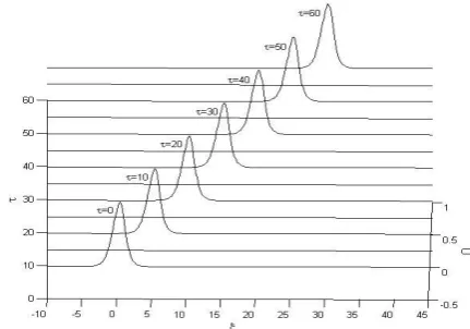
2. Case 2: Rapidly Varying Slope

When the variable topography is taken into account, the wave propagation in various topography are shown. The detailed amplitude variations are seen determined by the rapidly changing bottom profile. Figure 2 and 3 shows the wave propagation when the depth ℎ(𝜏)decreases rapidly. The depth profile is taken as

ℎ(𝜏) = {

_ℎ

ℎ

0

= 1.0

: 𝜏 < 50

1

= 0.64 : 𝜏 > 50

(19)

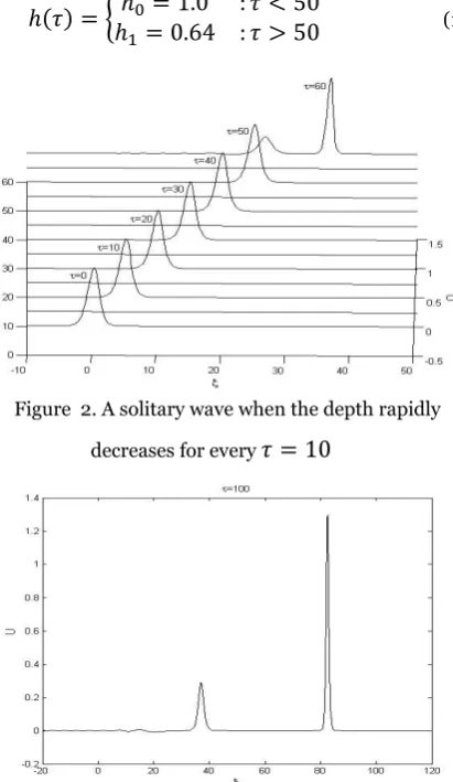
Figure 2. A solitary wave when the depth rapidly decreases for every 𝜏 = 10

Figure 3. A soliton followed by an oscillatory tail fissions into two solitons at =100when the depth rapidly decreases

From Figure 2 and 3, we can see that the solitary wave followed by an oscillatory tail fission into two solitons. Figure 2 shows the wave begin to fission and the amplitude of the waves begin to increase from 1 to 1.3 after 𝜏 = 50 following the depth condition while Figure 3 shows the wave propagate when

𝜏 = 100.

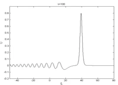
Here, a solitary wave disintegrate into several different sizes of solitary waves when it travels rapidly from a constant depth to another shallower constant depth, followed by small radiation tail depending on the depth variation. The process is called soliton fission and has been proven numerically and experimentally by Madsen and Mei (1969) while the analytical explanation was done by Tappert and Zabusky (1971) and Johnson (1973b).

On the other hand, Figure 4 and 5 shows the formation of a solitary wave when it is propagated over a rapidly increasing depth region for every

𝜏 = 10

and no fission of solitary wave is observed here. Instead, the solitary wave rapidly disintegrated and formed a radiation tail. The rapidly increasing depth profile is given as

ℎ(𝜏) = {

ℎ

0

= 1.0 : 𝜏 < 50

ℎ

1

= 1.3 : 𝜏 > 50

(20)

31 Figure 5. The numerical solution at =100. No soliton fission observed when a solitary wave propagates into rapidly

deeper area when the depth rapidly decreases

From the Figure 4, the amplitude of the solitary wave is begin to decrease from 1 to 0.8after

𝜏 = 50

following the depth condition. Meanwhile the wave propagation when 𝜏 = 100 is shown in Figure 5. As we can see the amplitude of the wave is decrease when the depth is increase and vice versa. Both Figure 3 and 5 are in a good agreement with previous research that at least one or more solitary waves are generated when propagates into a shallower water ℎ1< ℎ0. On the other hand, if the solitary wave propagates into a deeper region, ℎ1>ℎ0, then no other solitons are formed and the solitary wave decays into radiation (Johnson, 1973b; Grimshaw, 2007).

3. Case 3: Slowly Varying Slope

Next, we will take the opposite situation, in which the coefficients

𝜈(𝜏)

and

𝛿(𝜏)

in (5) vary slowly in which the solitary wave is propagating over a slowly changing topography. The solitary wave generally deforms adiabatically and there is a non-adiabatic response in the form of an extended small-amplitude secondary structure or a shelf, which can have a positive or negative polarity that travel behind the solitary wave (Grimshaw, 2007). From the depth profile,

ℎ(𝜏)

ℎ(𝜏) =

{

1 : 𝜏 < 100

(1 −𝛼(𝜏−100)₂ )2 : 100 < 𝜏 < 544.44, 𝛼 = 0.0009

0.64 : 𝜏 > 544.44

(21)

Figure 6. The amplitude of solitary wave increase adiabatically when propagating over a slowly shallower

region for every =100

Figure 7. A trailing shelf of positive polarity is formed behind the solitary wave as it propagates over a gradually

shallower region

Figure 6 shows the numerical simulation of the propagation of solitary wave over shallower region for every

𝜏 = 100

while Figure 7 shows the formation of a small-amplitude trailing shelf behind the solitary wave as it propagates over the shallower area when

𝜏 = 600.

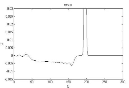
On the other hand, Figure 8 and 9 shows the numerical simulation of the formation of solitary wave into a deeper region for every

𝜏 = 100 and for 𝜏 = 500.

respectively. Here, the depth profile, h

( )

 is taken as

ℎ(𝜏) =

{

1 : 𝜏 < 100

(1 +𝛼(𝜏−100)

2 )

2

: 100 < 𝜏 < 411.5, 𝛼 = 0.0009

1.3 : 𝜏 > 411.5

32 Figure 8. The amplitude of a solitary wave propagating over

a gradually decreasing slope for every 𝜏 = 100 decreases adiabatically

Figure 9. A trailing shelf of negative polarity is formed behind the solitary wave as it propagates over a gradually

decreasing slope

The propagation of a small-amplitude trailing shelf behind the solitary wave as it propagates over the deeper region can

be observed in Figure 9 which is similarly happen when it propagate over the shallower region in Figure 7. Again, there is an excellent agreement with Grimshaw (2007).

V. CONCLUSION

The solitary wave propagation over a various background topography is tested. The configuration for the both rapidly and slowly changes of depth is studied. From the results, the solitary wave followed by an oscillatory tail has fission into few solitons as it travelled through rapidly decreasing depth. On the contrary, no soliton fission is observed when the wave propagates trough rapidly increasing depth. However, if the depth varies gradually, the solitary wave will disintegrate adiabatically and formed a trailing shelf. Similarly, for a slowly increasing slope, the trailing shelf will also disintegrate into secondary solitons, which is parallel to the process of soliton fission.

From the numerical results, we can see that the proposed numerical method using the PS method has been successfully used to solve both single KdV equation and also vKdV equation. It can be concluded that PS method is one of a good method to solve KdV type of equations as the result is in a good agreement with the previous studies.

VI. ACKNOWLEDGEMENT

The author would like to thank Universiti Malaysia Terengganu for providing funding support.

VII.REFERENCES

Chan, TF & Kerhoven, T 1985, ‘Fourier methods with

extended stability itervals for the Korteweg-de-Vries

equation’, SIAM Journal of Numerical Analysis, vol.

22, pp. 441-454.

El, GA, Grimshaw, RH & Wei, KT 2012, ‘Transformation

of a shoaling undular bore’, Journal of Fluid

Mechanics, vol. 709, pp. 371-395.

Grimshaw, R 1970, ‘The solitary wave in water of variable

depth’, Journal of Fluid Mechanics, vol. 42, no. 3, pp.

639-656.

Grimshaw, R 1971, ‘The solitary wave in water of

variable depth. Part 2’, Journal of Fluid Mechanics,

vol. 46, no. 3, pp. 611-622.

Grimshaw, R 1981, ‘Evolution equations for long, nonlinear internal waves in stratified shear flows’,

Studies in Applied Methamatics, vol. 65, pp. 159-188.

Grimshaw, R 2001, ‘Internal solitary waves’,

33 Grimshaw, R 2005, Nonlinear waves in fluids: Recent

advances and modern applications, Springer Wien,

New York.

Grimshaw, R 2006, ‘Internal solitary waves in a variable

medium’, GAMM-Mitt., vol. 30, no.1, pp. 96-109.

Grimshaw, R 2007, ‘Solitary waves propagating over

variable topography’, Tsunami Non. Waves, vol. 2, pp.

49-62.

Grimshaw, R, Pelinovsky, E & Talipova, T 2007,

‘Modelling internal solitary waves in the coastal ocean’,

Surveys in Geophysics, vol. 28, pp. 273-298.

Grimshaw, R, Pelinovsky, E, Talipova, T & Kurkin, A 2004,

‘

Simulation of the transformation of internal

solitary waves on oceanic shelves’, Journal of Physical

Oceanography, vol. 34, pp. 2774-2791.

Grimshaw, R, Pelinovsky, E, Talipova, T & Kurkina, O

2010, ‘Internal solitary waves: propagation,

deformation and disintegration’, Nonlinear Processes

in Geophysics, vol. 17, pp. 633-649.

Hilmi, D 2010,

‘

Weakly nonlinear waves in water of variable depth: Variable-coefficient Korteweg–deVries

equation’, Computers and Mathematics with

Applications, vol. 60, pp. 1747-1755.

Holloway, P, Pelinovsky, E & Talipova, T 2001, ‘Internal

tide transformation and oceanic internal solitary

waves’, Environmental Stratified Flows, vol. 3, pp.

29-60.

Johnson, RS 1973a, ‘On an asymptotic solution of the

Korteweg-de Vries equation with slowly varying

coefficients’, Journal of Fluid Mechanics, vol. 60, no. 4,

pp. 813-824.

Johnson, RS 1973b, ‘On the development of a solitary

wave moving over an uneven bottom’, Mathematical

Proceedings of the Cambridge Philosophical Society,

vol. 73, no. 1, pp. 183-203.

Kakutani, T 1971, ‘Effect of an uneven bottom on gravity

waves’, Journal of Physical Society of Japan, vol 30, no.

1, pp. 272-276.

Korteweg, DJ & de-Vries, G 1895, ‘On the change of form

of long waves advancing in a rectangular canal, and on

a new type of long stationary waves’, Philosophical

Magazine, vol. 39, no. 240, pp. 422-443.

Madsen, OS & Mei, CC 1969, ‘The transformation of a

solitary wave over an uneven bottom’, Journal of

Fluid Mechanics, vol. 39, no. 4, pp. 781-791.

Miles, JW 1980, ‘Solitary waves’, Annual Review of

Fluid Mechanics, vol. 12, pp. 11-43.

Miles, JW 1981a, ‘On internal solitary waves’, Tellus,

vol. 33, pp. 397-401.

Miles, JW 1981b, ‘The korteweg-de vries equation : a

historical essay’, Journal of Fluid Mechanics, vol.

106, pp. 131-147.

Ong, CT, Chew, YM & Tay, KG 2007, ‘Numerical

solution of the Burgers equation’, Advances in

Theoretical and Numerical Methods, Book Chapter

10.

Rashid, A 2006, ‘Convergences analysis of three-level

Fourier Pseudospectral Method for

Korteweg-de-Vries Burgers equation’, An International Journal

Computers and Mathematics with Applications, vol.

52, pp. 769-778.

Russell, JS 1845, ‘Report on waves’, Report of the 14th

Meeting of British Association for the

Advancement Science, pp. 311-390.

Tappert, FD & Zabusky, NJ 1971, ‘Gradient-induced

fission of solitons’, Physical Review Letters, vol. 27,

no. 26, pp. 1774-1776.

Tay, KG, Choy, YY, Tiong, WK, Ong, CT & Mohd, NY

2017, ‘Numerical solutions of the forced perturbed

Korteweg-de vries equation with variable

coefficients’, International Journal of Pure and

Applied Mathematics, vol. 112, no. 3, pp. 557-569.

Yuan, C, Grimshaw, R & Johnson, E 2018, ‘The

evolution of second mode internal solitary waves

over variable topography’, Journal of Fluid