Simulation Analysis of Dual Excitations Method for Improving the Sensitivity Distribution of an Electrical Capacitance Tomography System

(1)

*Corresponding author: [email protected]

10

Simulation Analysis of Dual Excitations Method for

Improving the Sensitivity Distribution of an Electrical

Capacitance Tomography System

Muhammad Safwan Senen

1

, Elmy Johana Mohamad

1

*, Hanis Liyana Mohmad

Ameran

1

_{, Ruzairi Abdul Rahim}

1

_{, Omar Faizan Marwah}

2

_{, Siti Zarina Mohd}

Muji

1

1_{Faculty of Electrical and Electronic Engineering}

Universiti Tun Hussein Onn Malaysia, 86400 Batu Pahat, MALAYSIA 2_{Faculty of Mechanical and Manufacturing Engineering}

Universiti Tun Hussein Onn Malaysia, 86400 Batu Pahat, MALAYSIA

Received 8 February 2017; accepted 8 March 2017, available online 9 March 2017

1. Introduction

Tomography is a method to image the cross-section of an enclosed region by measuring the internal characteristics of the specified domain [1]. Tomography systems usually consist of non-intrusive sensors placed around the periphery of an object in the container [2]. The development of tomographic instrumentation, started in the 1950’s, and has led to the widespread availability of body scanners which is part of modern medicine nowadays. Process tomography evolved essentially during the mid-1980 [2]. The development of this technology was first discovered in 1950’s which known as Muon tomography that uses cosmic rays muon for imaging magma chamber that’s can determine prediction of volcanic eruptions. In 1953, planography which had almost the same concept of tomography discovered and being explained in the medical journal. Development of tomography had reach on the computer assisted tomographic technique in the mid to late 70s

.

There are two ways of installing the electrodes: in the inside or on the outside of the pipe. The location of the electrode whether internal or external is chosen by considering the material of the pipe wall. If the pipe wall is a conductor, the sensor should be installed inside as the

electrical field inside the sensor will always increase in proportion to the material permittivity when the sensor is filled uniformly with higher permittivity material [3]. For non-conducting pipe walls, the sensor can be installed both inside and outside of the pipe. Internal electrodes will give linear characteristic to the reading as when placed inside the pipe, the electrodes could endure extremely high pressure, temperature and turbulences. In choosing the internal electrode type, the characteristic of the flow material in the pipe needs to be considered.

External electrodes design on the tomography system is comparatively simpler to install and easier to fabricate [4]. Since the electrodes is outside the pipe, the material flow inside the vessel would not affect the electrodes. However, external electrodes often provides nonlinear reading as the pipe material and thickness have impact on the measurement.

In this work, an Electrical Capacitance Tomography (ECT) system with 16 external electrodes is used to image liquid/gas flow. In an ECT system, the capacitance value between electrodes is measured to determine the permittivity distribution of the materials inside the pipe. As each material have different permittivity value, ECT can reliably differentiate various materials. ECT has been

Abstract: A well-known challenge in using an Electrical Capacitance Tomography (ECT) system to obtain

cross-section image of pipelines is the system’s non-uniform sensitivity distribution where the system is less sensitive at the pipe’s centre compared to the pipe’s wall proximity. A method to overcome this issue is by using two The aim of this work is to analyse the sensitivity map distribution by using two excitation potentials technique (1) to observe the changes of the inter-electrode capacitance and the permittivity of the dielectric material, (2) to investigate the distribution of electrical potential at the centre of the pipe, also (3) to investigate the feasibility of two excitation potentials technique to improve the sensitivity map in ECT system. The COMSOL Multiphysics software is used to simulate an ECT system to obtained results by generated phantoms, measured values such capacitance value and electrical potential, also for the sensitivity map distribution in the pipe model. By using this technique, an improvement is made on the sensitivity map distribution in the central area.

(2)

11

successfully applied in various industries as it is reliable, robust, fast and inexpensive [5-6].

However, in addition to the nonlinear measurement provided by the external electrodes, another shortcoming of an ECT system is that its low image resolution caused by the soft field effect where its sensor’s sensitivity depends greatly to the location of the object. The ECT inter-electrode projections are curved towards the wall proximity, making the sensor less sensitive in the central area of the pipe. As the electrode arrangement is in a circular array, the decrease of electrode surface area per unit axial length reduces the inter-electrode capacitance measurement [7].

In this paper, we present a simulative analysis of applying the dual excitations method in a 16-electrode ECT system and compare the results of using the conventional single excitation method. The dual excitations method is used in order to increase the system’s sensitivity around the central area of the pipe by applying different excitation potential level in accordance to the position of the source and receiving electrodes.

2. Methodology

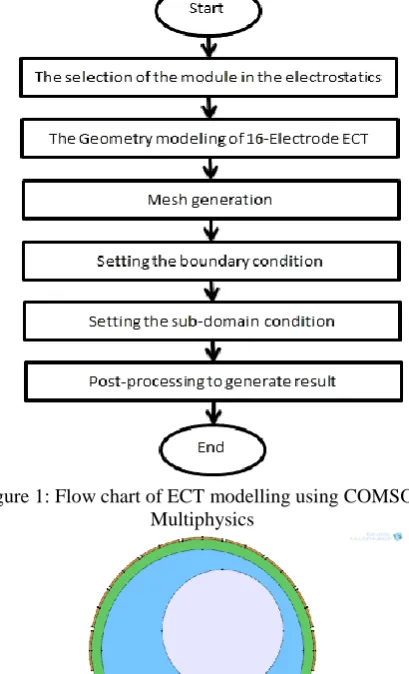
Figure 1 shows the flow chart of the modelling process of the ECT system using Finite Element Analysis (FEA) software named COMSOL Multiphysiscs. The module consists of several physics properties and applications such as electrostatics, magnetostatics, and electromagnetic quasi-statics; complete with access to any derived field quantities and couplings to other physics [8]. Since ECT consists of capacitors as the electrodes, electrostatic module is chosen for the module.

The performance of capacitors, inductors, motors, and microsensors can be evaluated using the AC/DC Module. Principally, all the devices can be characterized as electromagnetics; yet the influences of other types of physics cannot be neglected. For example, thermal effect can change a material’s electrical properties.

The ECT system model that will be used consist of 16-electrodes array mounted at the periphery of an acrylic pipe with a diameter of 100 mm pipe and wall thickness of 5 mm, while the electrode stretch angle, θ is 22.5°. For this project, the focus is on the numerical modelling of the ECT system to simulate the electrical field and electrical potential.

A Mesh is a partition of the geometry model into small units of simple shapes. The finite element mesh is very important in a numerical simulation analysis. A finer finite element mesh commonly gives better calculation results. The COMSOL Mulitphysics mesh generation will subdivide of the domains of a geometric model into triangles (2D) or tetrahedral (3D). The mesh is created automatically to a set scale, and it can be refined automatically or adaptively in any specified regions.

The boundary setting is a procedure to interpret the physical analysis. The setting of boundaries can differentiate the boundaries between different materials as well as between material and the environment. Each material have its own permittivity which will affect in the results. The pipe permittivity must be set higher

permittivity than the material tested in the pipe because to prevent the potential different excited in the electrode does not pass through the pipe since the electrode are arrange outside the pipe.

As the transmitter electrodes is being excited with certain value of potential difference, the remaining electrodes are set to zero potential or grounded. This is to set the remaining electrodes to become receiver electrodes.

Next, the sub-domain of materials inside the pipe is determined by including the dielectric constant permittivity for instance air and water.

Figure 2 shows an example of the pipe system model where the pipe is filled with different materials. The blue colour represent water which have permittivity of 80.8 and the white colour represent air which have permittivity of 1. The sub-domain dielectric value is assumes to be constant throughout the material.

Post processing is an application to plot any model quantity and characteristics based on the boundary and sub-domain setting earlier. Specifically for this project, the 2D image reconstruction is expected with the distribution of electrical field and potential for the pipe cross section.

Figure 1: Flow chart of ECT modelling using COMSOL Multiphysics

(3)

12

2.1 Single Excitation Method

Firstly, we simulate the model using the single excitation potential method. The value of potential difference used as excitation source is 4 V. The value of potential difference can be used any but choosing 4V because to get the smaller value to check the differences between the single excitation potential and the dual excitations methods. From the simulation, obtain the electric field lines which is deflected as it passing through a different material also the sensitivity map distribution.

Figure 3: Electric field simulation for single excitation potential

2.2 Dual excitations Method

Then, we proceed to apply dual excitations method on the same modelling. The electrical potential value for the dual excitations method is 4V and 3V. This two value is determined after done many simulation with different value [9 – 11]. Obtained results as in the single excitation and compared the differences in the result obtained.

Figure 4: Electric field simulation for dual excitations method

3. Simulation Results

3.1 Electric Field Simulation

3.1.1 Electric potential distribution

Based on the simulation, the electric field distribution is represented as line while the electrical potential is indicated by colored contour or colored surface. The level of the electrical potential is differentiate of the color represented which is for the highest value will be red while the lowest value will be blue.

The differences between single and dual excitations method on the electrical potential in ECT is the coverage of the electrical potential value in the center of the pipe is shown in Table 1.

Table 1 Electric field simulation comparison between single excitation and dual excitations method

Single excitation method Dual excitations Method

3.1.2 Potential Difference (V) distribution in

each electrode

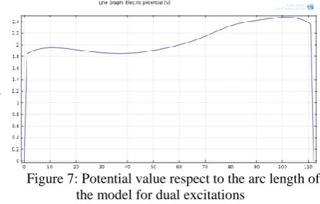
With COMSOL Multiphysics, we can obtain value of potential difference between each electrode pair by using the boundary probe placed on the electrode of the model. The boundary probe is used to calculate the average value of potential in a surface line of the electrode.

Figure 6 and 7 show the reading of potential difference in respect to the arc length of the model used for single excitation and dual excitations method respectively.

Figure 6: Potential value respect to the arc length of the model for single excitation

(4)

13

3.1.3 Capacitance value for each electrode

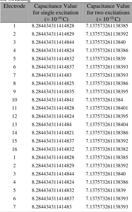
To obtain the value of the capacitance, we use the domain probe since the value of the capacitance in the electrode is measured by the whole electrode.

Table 2 Capacitance reading on each electrode for different excitation method (between single and multiple) for switching

Electrode Capacitance Value for single excitation

(× 10-10 _C)

Capacitance Value for two excitations

(× 10-10 _C)

1 8.284434311414828 7.137573261138385 2 8.284434311414829 7.137573261138392 3 8.284434311414844 7.13757326113840 4 8.284434311414824 7.137573261138386 5 8.284434311414832 7.13757326113839 6 8.284434311414837 7.137573261138393 7 8.28443431141483 7.137573261138393 8 8.284434311414825 7.137573261138386 9 8.284434311414835 7.137573261138395 10 8.284434311414841 7.1375732611384 11 8.284434311414828 7.137573261138401 12 8.284434311414824 7.137573261138395 13 8.28443431141484 7.137573261138404 14 8.284434311414821 7.137573261138386 15 8.284434311414837 7.137573261138392 16 8.284434311414832 7.137573261138382 1 8.284434311414828 7.137573261138385 2 8.284434311414829 7.137573261138392 3 8.284434311414844 7.13757326113840 4 8.284434311414824 7.137573261138386 5 8.284434311414832 7.13757326113839 6 8.284434311414837 7.137573261138393 7 8.28443431141483 7.137573261138393

3.2 Sensitivity Maps

3.2.1 Electrical Potential Sensitivity Map

The sensitivity map shows the electrical potential in each pixel of the ECT geometry when the pipeline contains homogenous medium which is air in this case. The potential sensitivity distribution in the pipe are shown in Figure 8 and Figure 9 for single excitation method and dual excitations method respectively. As it shows, the distribution is more uniform for the dual excitations than the single excitation since in the single excitation the potential value decreases greatly as it gets farther from the excitation electrode.

Figure 8: Electrical Potential (V) sensitvity map for single excitation for switching 1

Figure 9: Electrical Potential (V) sensitvity map for two-differential excitation for switching 1

3.2.2 Electric

Displacement

Field

Normalization Sensitivity Map

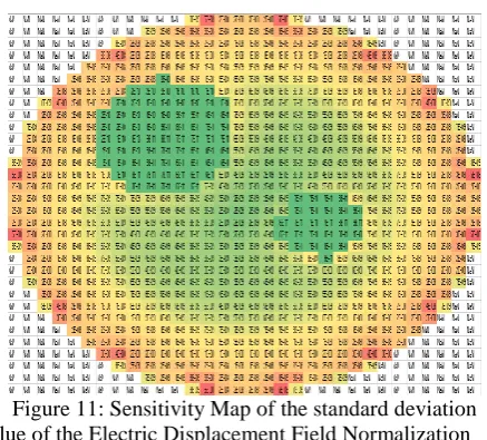
The results will be different between electric displacement field normalization sensitivity map (C/m^2) and potential difference (V) sensitivity map of the same model. This is because the value of capacitance (C) is affected by the value of permittivity ( ) of the medium or substance in the pipe.

As the result, the higher permittivity proportionally with the electric field, it show higher value of the distribution electric displace displacement field normalization (C/m^2) for each pixels in the sensitivity map. Therefore, substance or medium inside the pipe could be recognize and the forming of the phantom that represent the foreign medium or substance can be seen.

To obtain the result, the sensitivity map of each switching must be gathered first (switching 1 to switching 16).

(5)

14

(1) After undergoes the calculation of each pixels, the results is compared between the single excitation and the dual excitations technique. Figure 10 shows the results after the calculation had been made for both excitation modes.

From both reading we can compare that the sensitivity map for the dual excitations technique have better reading since the number of pixels represent the phantom on the right side is lower in the single excitation than the dual excitations .

A higher resolution of the sensitivity map will shows the phantoms for the single excitation is not too accurate rather than the dual excitations.

Figure 10: Sensitivity Map of the standard deviation value of the Electric Displacement Field Normalization

for Single Excitation Technique

Figure 11: Sensitivity Map of the standard deviation value of the Electric Displacement Field Normalization

for dual excitations Technique

3.3 Error Calculation

To check the error of the simulated measurements, some equations had been developed. The calculations involved focused on the area of water inside the pipe. The equation will be:

(2)

Based on the normalization image, the number of pixels of the pipe are 812 pixels. The area of pixel is then calculated by using below equation:

(3) Then, calculate the area of water according to the normalization image formed and also the water simulation model. Below shows the calculation for single excitation:

Below shows the calculation for dual excitations:

For single excitation the error calculation by using the equation is:

4.09%

While for dual excitations the error calculation by using the equation is:

4.08%

As we can see that the error reading for dual excitations had lower 0.01% than for single excitation. If the resolution for the sensitivity map is increase maybe a higher differences in error reading could be observe.

The ideal simulation is where the error calculation is equal to 0%, which indicates that the simulation results is exactly the same with the model.

4. Conclusion

(6)

15

process time for the switching also enhance the image reconstruction such been done in previous studies [12] which shows that segmented excitation can perform better for inspections in closed region.

The reconstruction of sensitivity map by using COMSOL Multiphysics also can be link with other software such as Microsoft Excel and MATLAB which helps to get advance analyzing on the characteristic of ECT. The sensitivity map is uses to analyze the ECT characteristic whether it is acceptable from the researched that already been done, and error in the simulation compare to the actual could be calculated [8]. In the error calculation, there is an improvement which is 0.01%.

Acknowledgments

The authors are grateful to the financial support from Research University Grant of Ministry of Education Malaysia: Research Acculturation Collaborative Effort 1519 and UTM Matching Grant M03.

References

[1] D. Watzenig and C. Fox, “A review of statiscal modelling and inference for electrical capacitance tomography” in Measurement Science and Technology, Volume 20, Number 5.

[2] L. Jing, S. Lu, L. Zhihong, S. Meng “An image reconstruction algorithm based on the extended Tikhonov regularization method for electrical capacitance tomography” in Measurement, Volume 42, Issue 3, April 2009, Pages 368 – 376.

[3] E. J. Mohamad, O. F. Marwah, R. A. Rahim, L. P. Ling, “An analysis of sensitivity distribution using two differential excitation potentials in ECT” in 2011 Fifth International Conference on Sensing Technology Proceeding.

[4] S. M. Din, “Investigation of segmented excitation of electrical capacitance tomography (ECT)” in unpublished Thesis, Universiti Teknologi Malaysia, July 2014

[5] S. S. Donthi, "Capacitance based Tomography for Industrial Applications”, EE Dept. IIT Bombay, 2004.

[6] R. A. Williams and M. S. Beck, Process Tomography: Principles, Techniques, and Applications: Butterworth-Heinemann, 1995.

[7] Z. Fan, R. X. Gao, and J. Wang, "Virtual Instrument for Online Electrical Capacitance Tomography," in Practical Applications and Solutions Using LabVIEW, Intech, 2011, pp. 3-16.

[8] N. Bahrani, "2 1/2 D Finite Element Method for Electrical Impedance Tomography Considering the Complete Electrode Model," M.Eng, Electrical and Computer Engineering, Carleton University, Canada, 2012

[9] A. M. Olmos, M. A. Carvajal, D. P. Morales, A. García, and A. J. Palma, "Development of an Electrical Capacitance Tomography system using four rotating electrodes," Sensors and Actuators A: Physical, vol. 148, pp. 366-375, 2008.

[10]K. J. J. Alme and S. Mylvaganam, "Comparison of Different Measurement Protocols in Electrical Capacitance Tomography Using Simulations," IEEE Transactions on Instrumentation and Measurement, vol. 56, pp. 2119-2130 2007.

[11]L. Peng, J. Ye, G. Lu, and W. Q. Yang, "Evaluation of Effect of Number of Electrodes in ECT Sensors on Image Quality," Sensors Journal, IEEE, vol. 12, pp. 1554-1565 2012.

[12]P. T. Ltd., “Electrical capacitance tomography system type TFLR5000 operating manual,