Point Information Gain and Multidimensional Data Analysis

Point Information Gain and Multidimensional

Data Analysis

Renata Rychtáriková1,*, Jan Korbel2, Petr Macháˇcek1, Petr Císaˇr1, Jan Urban1and Dalibor Štys1 1 _{Institute of Complex Systems, South Bohemian Research Center of Aquaculture and Biodiversity of}

Hydrocenoses, FFPW, University of South Bohemia in ˇCeské Budˇejovice, Zámek 136, Nové Hrady 37333, Czech Republic; [email protected] (P.M.); [email protected] (P.C.); [email protected] (J.U.); [email protected] (D.S.)

2 _{Faculty of Nuclear Sciences and Physical Engineering, Czech Technical University in Prague, Bˇrehová 7,}

Prague 15519, Czech Republic; [email protected]

* Correspondence: [email protected]; Tel.: +420-387-773-833

Abstract: We generalize the point information gain (PIG) and derived quantities, i.e., point information gain entropy (PIE) and point information gain entropy density (PIED), for the case of the Rényi entropy and simulate the behavior of PIG for typical distributions. We also use these methods for the analysis of multidimensional datasets. We demonstrate the main properties of PIE/PIED spectra for the real data on the example of several images, and discuss further possible utilizations in other fields of data processing.

Keywords: pointinformationgain;Rényientropy; dataprocessing

1. Introduction

Measurement of relative information between two probability distributions is one of the most important goals of information theory. Among many other concepts, there are two, which are widely used. By far the most widespread concept is called the relative Shannon entropy or the Kullback–Leibler divergence. In this work, we rather use an alternative approach based on a simple concept of entropy difference. By generalization of both concepts from Shannon’s approach to Rényi’s approach, we obtain the whole class of information variables that enables to aim to different parts of probability distributions and interpret it as an investigation of different parts of multifractal systems. Despite the mathematical precision of the concept of the Shannon/Rényi divergence, we use another concept, the (Rényi) entropy difference, for introduction of a value which locally determines an information contribution of a given element in a discrete set. Even though there is no substantial restriction on the usage of a standard divergence for calculation of the information difference upon elimination of one element from a set, for practical reasons, we used the simple concept of entropy difference between sets with and without a given element. The resulted value has been called a point information gainΓ(αi)[1,2]. The goal of this article is to examine and demonstrate some properties of this variable and derived another quantities, namely a point information gain entropyHαand a point information gain entropy densityΞα. We also introduce the relation of all these variables to global and local information in multidimensional data analysis.

2. Mathematical Description and Properties of Point Information Gain

2.1. Point Information Gain and Its Relation to Other Information Entropies

An important problem in the information theory is to estimate the amount of information gained/lost by refining/approximating the probability distributionPby the distributionQ. The most popular measure used in the theory is the Kullback–Leibler (KL) divergence, defined as

DKL(P||Q) =

∑

pjln

pj

qj

whereSP(Q)is so-called cross-entropy [3] andS(P)is the Shannon entropy of distributionP. IfPis similar toQ, this measure can be approximated by entropy difference

∆S(P,Q) =S(Q)−S(P). (2)

Indeed, this measure does not obey as many theoretic-measure axioms as the KL-divergence. For instance, forP6=Qwe can still obtain∆S(P,Q) =0. Nevertheless, ifP≈QandP6=Q, this value can be still a suitable quantity revealing some important information aspects of a system. The situation, when the distributions are approximative histograms of some underlying distributionsPfornand (n+1) measurements, respectively, is particularly interesting. In this case, the entropy difference

∆S(Pn,Pn+1) =S(Pn+1)−S(Pn) (3)

can be interpreted as an information gained by the (n+1)-th measurement. Naturally, Pn → P. When dealing with real complex systems, it is sometimes advantageous to introduce new information variables and entropies that capture the complexity of the system better, e.g., Hellinger’s distance, Jeffrey’s distance or J-divergence. There are also some specific information measures that have special interpretations and are widely used in various applications [4,5]. Two most important quantities are the Tsallis–Havrda–Charvát (THC) entropy [6], which is the entropy of non-extensive systems, and the Rényi entropy, the entropy of multifractal systems [7,8]. The latter is tightly connected to the theory of multifractal systems and generalized dimensions [9]. It is defined as

Hα(P) = 1

1−αln

∑

α

j, α≥0, (4)

where α is the Rényi coefficient and pj is the probability of occurrence of a phenomenon j in the discrete distribution. Limit α → 1 recovers the Shannon entropy. Similar to the Shannon entropy, the Rényi entropy has also an operational meaning. Actually, it can be interpreted as the average information cost, when the cost of an elementary information is an exponential function of its length [10]. Thus, changing the parameter α changes the cost of the information and therefore accentuates some parts of the probability distributions while suppressing the other. Thus, by taking into account the whole class of Rényi entropies, we get a new generalized class of information quantities.

The point information gainΓ(αi)of thei-th point was developed as a practical tool for assessment of the information contribution of an element to a given discrete distribution [11]. Similar to the Shannon entropy difference, it is defined as a difference of two Rényi entropies—with and without the examined element of a discrete phenomenon. Let us consider a discrete distribution ofkdistinct possible outcomes (e.g., different colors of pixels). Let us have a discrete distribution

P={pj}kj=1=

nn₁ n, . . . ,

ni

n, . . . , nk

n o

, (5)

where n denotes the total number of elements in the discrete distribution and ni the number of elements ofi-th phenomenon,i ∈ {1, 2, ...,k−1,k}, respectively. Let us denoten(_ji) = nj for j 6= i andn(_ii)=ni−1. Then the distribution with the omittedi-th phenomenon can be written as

P(i)=np(_ji)ok

j=1=

( n(₁i) n−1, . . . ,

n(_ii) n−1, . . . ,

n(_ki) n−1

)

Hence, we may write the point information gain Γ(αi) as (in the text we use the natural logarithm to simplify calculations. However, all computations have been performed with the usage of binary logarithm which, for the Rényi entropy and its derivatives, yields values in bits.)

Γ(i) α =Hα

P(i)−Hα(P) = 1 1−αln

k

∑

j=1

p(_ji)α

! − 1

1−αln

k

∑

j=1

(pj)α

!

= 1

1−αln 

 

∑k j=1

p(_ji)α ∑k

j=1pαj





, (7)

wherekis the total number of the phenomena in the discrete distribution. In contrast to the commonly used Rényi divergence [12–18], we use Γ(αi) for its relative simplicity and practical interpretation. Unlike the KL divergence, the Rényi divergence cannot be interpreted as a difference of cross-entropy and entropy of the underling distribution and computation becomes intractable. As discussed above, for similar distributions, it still preserves its information values.

After the substitution for the probabilities, one gets that

Γ(i)

α =

1 1−αln

∑k j=1

n(_ji)α (n−1)α

∑k j=1

nα j

nα

=Cα(n) + 1 1−αln

∑k j=1

n(_ji)α ∑k

j=1nαj

, (8)

whereCα(n) =ln n−n1

₁₋α_α

depends only onn. Forn→∞andΓ(αi)→0, the whole entropy remains finite (contrary to unconditional entropy, which has to be renormalized for continuous case, for details see Reference [7]). Therefore we examine only the second term. When the argument of the logarithm is close to 1, i.e.,

k

∑

j=1

n(_ji)α≈

k

∑

j=1

nα

j, (9)

which leads to the condition that

n(_ii) ni

!α =

ni−1

ni

α

≈1, (10)

for given α, one can then approximate the logarithm by the Taylor expansion of the first order. After denoting

Dα(i)=

∑k j=1

n(_ji)α ∑k

j=1nαj

, (11)

the second term ofΓ(αi)can be approximated as

1 1−αlnD

(i)

α =

1 1−α

Dα(i)−1

+O

D(αi)−1

2

, (12)

We shall continue by utilizing the Rényi entropy due to its relation to the generalized dimension of multifractal systems [20,21]. Let us concentrate again to the termD(_αi). We can rewrite it as

D(_αi)= ∑

k j=1

n(_ji)α ∑k

j=1nαj

= ∑

k

j=1,j6=inαj + (ni−1)α

∑k j=1nαj

=1−α n

α−1 i

∑k j=1nαj

+ 1

∑k j=1nαj

ω

nα−2 i

. (13)

where we use the smallωasymptotic notation. Specifically, providedα=2, we obtain

Γ(i)

2 ≈ C2(n) + 1 1−2



 ∑k

j=1,j6=in2j + (ni−1)2

∑k j=1n2j

−1 

≈ C2(n) + 2ni

−1 ∑k

j=1n2j

, (14)

which explains why the dependencyni onΓ(2i)is approximately linear (Figure2d). In general, point information gain is a monotone function ofni, respectivelypi, for all possible discrete distributions. Thus, it may be used as a quantity of information gain between two discrete distributions, which in the occurrence of one particular feature differ.

Let us discuss an interpretation of the point information gain. We can rewrite Equation (8) as

Γ(i) α =ln

n n−1

₁₋α_α +ln



1+

(ni−1)α−nαi

∑k j=1nαj



 1 1−α

=−ln

1− 1 n

α1−1α

+ln 

 1+n

α i

1− 1

ni

α

−1

∑k j=1nαj



  1 1−α

. (15)

We are interested in the situation whenΓ(αi)=0. After straightforward manipulations, we can get rid of ln and₁₋1_αpower, so

1−1

n α

=1+nα i

1−_n1

i

α

−1

∑k j=1nαj

. (16)

Ifn 1 andni 1, we can approximate both sides with the rule(1+x)α ≈ 1+αx forxclose to zero which gives

1− α n =1−

αnα_i−1 ∑k

j=1nαj

. (17)

Thus we end with

ni=

α−1 s

∑k j=1nαj

n . (18)

This shows that Γ(αi) = 0 holds for events with average frequency. Γ (i)

α < 0 corresponds to rare events, while Γ(αi) > 0 corresponds to frequent events. Thus, in addition to the definition of the quantity of the contribution of each event to the examined distribution, we also obtain the discrimination between points which contribute to the total information of the given distribution under the statistical assumption represented by a particularα. This opens the question on existence of the “optimal” distribution for the givenα.

Then, the possible variants of such optimality arise subsequently: The first one can be defined as a distribution for which exactly a half of the valuesniproducesΓ(αi)> 0 and the other half yields

Γ(i)

α < 0. The second one requires values Γ (i)

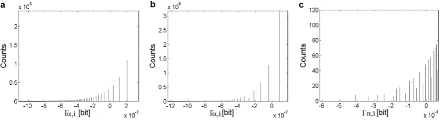
With respect to the previous discussion and practical utilization of this notion, we emphasize that for real systems with large n are values Γ(αi) relatively small numbers for current numerical precision of common computers. Their further computer averaging and numerical representation lead to significant errors such as underflow and overflow (e.g., Figure1c). At lower values α, the valuesΓ(αi)are broadly separated for rare points, while, at higher valuesα, the resolution is higher for more frequent data points. Therefore, spectrumΓ(αi)vsαis more advisable to compute rather than a singleΓ(αi)value at a chosenα.

2.2. Point Information Gain for Typical Distributions

In Figure1, we demonstrateΓ(αi)-transformations of three thoroughly studied distributions—the Lévy, Cauchy, and Gauss distribution (specified in Section5.1). Mainly Figure1c shows averaging of digital levels which results in multiple appearance of unique points. This phenomenon is reduced with the increasing number of the points in the distribution, nevertheless, it does not disappear in any real case. Thus, the monotone dependencies ofni, respectivelypi, on theΓ(αi)are valid only at the approximation to an infinite resolution in levels of values.

Figure 1.Γ_α,i-transformations of the discretized Lévy (a), Cauchy (b), and Gauss (c) distribution atα = 0.99. The deviation from the monotone dependency in the Gauss distribution is due to the digital rounding.

Figure2shows distribution changes of the valuesΓ(αi)with the increasingα-parameter. For each parameterα, the elementsΓ(αi)are enveloped by monotone increasing curves. For instance, as devised in Equation (14), the near linearity of the dependency of the number of elements on the valuesΓ(αi)at

Figure 2. Γ(αi)-transformations of the discretized Lévy distribution atα={0.5, 0.99, 1.5, 2.0, 2.5, 4.0}

(fromatof).

2.3. Point Information Gain Entropy and Point Information Gain Entropy Density

During the previous sections we showed thatΓ(αi) is different for any ni and the dependency of these two variables is a monotone increasing function for all α > 0. Here, we propose new variables—a point information gain entropy (Hα) and point information gain entropy density (Ξα) defined by formulas

Hα= k

∑

j=1

njΓ(αj) (19)

and

Ξα= k

∑

j=1

Γ(j)

α . (20)

They can be understood as a multiple of the average point information gain and—under linear averaging—an average gain of the phenomenonj, respectively.

The next question is whether theΞαhas some expected properties. In this aspect, we mention the fact observed upon examination of Equation (12), which enable us to rewrite it as

Ξα= k

∑

j=1

Γ(j)

α =

k 1−αln

_nα

(n−1)α

+ 1

1−α

k

∑

i=1 ln



 ∑k

j=1,j6=inαj + (ni−1)α

∑k j=1nαj



=

=Cα(n)·k+ 1 1−αln

k

∏

j=1

D(_αj) !

, (21)

where the product in the argument of the logarithm in the second term is a product of functions upper limited by 1 and thus again a function upper limited by 1. From the previous analysis done for theD(_αi), we may conclude that the point information gain entropy density (Ξα) inherits properties of Rényi entropy, i.e., zooming properties, etc.

Similar to Equation (21), the point information gain entropy (Hα) can be rewritten as

Hα = k

∑

j=1

njΓ(αj)=

∑k j=1nj 1−α ln

_nα

(n−1)α

+

k

∑

i=1

niln





(_∑k_j=1,j6=inα

j + (ni−1)α)

∑k j=1nαj



=

=Cα(n)· k

∑

j=1

nj+ln k

∏

j=1

D(_αj)nj

!

. (22)

Again, the argument of the logarithm in the second term is upper limited by 1. The Hα has also properties inherited from Rényi entropy, although their mutual relation is more complicated.

3. Estimation of Point Information Gain in Multidimensional Datasets

3.1. Point Information Gain in the Context of Whole Image

Input:n-bin histogramh;α, whereα≥0∧α6=1 Output:Γα;Hα;Ξα

1 p=h/sum(h); % explain the frequency histogramhas a probability histogramp 2 Γα=zeros(h); % create a zero matrixΓαof the size of the histogramh

3 fori=1tondo

4 h₂=h; % create a vectorh₂identical to the histogramh 5 if h₂(i)6=0then

6 h2(i) =h2(i)−1;

% if the bin i of the histogramh2is occupied, remove an element at the position i 7 end

8 p₂=h2/sum(h₂); % calculate a probability histogramp₂without the examined element 9 Γ(_αi)= ₁₋1

αlog2(sum(p2. ∧

α)/sum(p.∧α));

% calculateΓ(αi)as a difference of two Rényi entropies – with and without the examined element,

respectively Equation(7)) 10 end

11 H_α=sum(h.∗Γα);

% calculate Hαas a sum of the element-by-element multiplication ofhandΓα(Equation(19))

12 Ξ_α=sum(Γα); % calculateΞ_αas a sum of all unique values inΓα(Equation(20));

Algorithm 1:Point information gain vector (Γα), point information gain entropy (Hα), and point information gain entropy density (Ξα) calculations for global (Whole image) information and typical histograms.

For each parameter α, the calculation of Γ(_αi) helps to find values of the intensities with the identical occurrences and determine their distribution in (a structural part of) the image. Thus, in general, the recalculations toΓ(αi)can be considered as Look-up Tables—intensities with the highest probabilities of occurrences in an image correspond to the highest (positive) values Γ(αi) and the brightest intensities in aΓ(αi)-transformed image and vice versa. Sometimes, mainly in case of local information, due to the transformation of the original valuesΓ(αi)into an 8-bit resolution, some levels

Γ(i)

α are merged into one intensity level of the transformed image.

Everything is best visualized in Figures 3–4 which show the Γ(αi)-transformations of the texmos2.s512 image. The intention was probably to create an image with a uniform distribution of intensities. Provided the uniform intensity distribution, the output of the globalΓ(αi)-calculation would be only one value Γ(αi), i.e., Figure 3b would be unicolor. However, 8 original intensities (Figure3a) resulted in five valuesΓ(_0.99i) (i.e., local parts) (Figure4b,d). The detailed image analysis showed that the number of occurrences is only identical for intensities 32-224 and 96-128-192, i.e., there are five unique values of frequencies of intensity occurrences (Figure 4a). For a change, in the 4.1.07 image, the global Γ(_0.99i) -recalculation emphasizes the unevenness of the background and shadows around a group of the jelly beans (Figure 5b). In conformity with the statement in the next-to-last paragraph in Section2.1, this principle also enables to highlight rare points in much more intensity richer images, mainly at lowα-values. The calculations using higher valuesαmerge resulted Γ(i)

Figure 3. Γ_0.99(i) -transformations of the texmos2.s512 image [26]. Original image (a) and information images calculated from the whole image (b), a cross around each pixel (c), and squares of the side of 5, 15, and 29 px, respectively, with the centered examined pixel (d–f).

Figure 4. Histograms ofΓ(_0.99i) -transformations of the texmos2.s512 image [26]. Original image (a),

original valuesΓ(_0.99i) calculated from the whole image (b), original valuesΓ(_0.99i) calculated from a cross

whose shanks intersect in the examined pixel (c),Γ(_0.99i) -transformed images calculated from the whole

Figure 5. Γ(_0.99i) -transformations of the 4.1.07 image [26]. Original image (a) and information images calculated from the whole image (b), a cross around each pixel (c), and circles of the diameter of 5, 17, and 30 px, respectively, with the centered examined pixel (d–f).

3.2. Local Point Information Gain

Since multidimensional datasets, as e.g., images, consist of special structures given by the pixel lattice, it can be also beneficial to calculate not only global information gain, but also local information gain in some defined surroundings (Algorithm 2). The local information is defined after removing an element from the bin i where the element lies in the center of the surroundings which creates the intensity histogram. The choice of the local surroundings around pixels is specific for each image. However, we do not have any systematic method for comparison of suitability of different surroundings around the pixels. The suitability of the chosen surroundings depends obviously on the process by which the observed pattern or other distribution was generated. According to our knowledge, the choice of the appropriate surroundings on the basis of known image generation was studied only for cellular automata [28–30]. This makes the study of the local information very interesting, because it outlines another method for recognition of the processes of self-organization/pattern formation [31]. In this article, we confine ourselves on the usage of the local information for better understanding both the limitation of the method of the Γ(αi)-calculation and the local information itself. The cross, square, and circular surroundings around each pixel are demonstrated on three different standard images—texmos2.s512 (monochrome, computer-generated, unifractal), 4.1.07 (RGB, photograph, unifractal) [26], and wd950112 (monochrome version, computer-generated, multifractal) [27].

The cross from the intensity values, whose shanks meet in the examined point of the original image [1], was chosen as the first local surroundings. In contrast to the global recalculation, such a transformation of the texmos2.s512 image produces a substantially much intensity richerΓ(αi)-image. One can see that a relatively simple global information consists of a more complex local information (Figure4a,c,e).

rather recommended to use. As seen in Figure5d–f, the increase of the diameter up to the size of the jelly beans reduces the background gradually. The next increase enables to group the jelly beans into higher-order assemblies. A similar grouping is observable for the smallest squares in the transformed texmos2.s512 using the 29-px square surroundings (Figure3f). In contrast, lower values of square surroundings (Figure3d) highlight only the border intensities.

Input: 2-D discrete dataIm×n;α, whereα≥0∧α6=1; parameters of surroundingsa,b Output:Γ(αi);Hα;Ξα

1 Γα=zeros(I); % create a zero matrixΓαof the size of theI_m×nmatrix

2 hashMap=containers.Map; % declare an empty hash-map (the key-value array) 3 fori= (a+1)to(m−a−1)do

4 forj= (b+1)to(n−b−1)do 5 h=getHist(I(i,j));

% create a histogramhfrom the elements around the pixel (i,j) ofIm×n

6 p=h/sum(h); % explain the histogramhas a probability histogramp

7 h(I(i,j)) =h(I(i,j))−1; % remove the examined point (i,j) from the histogramh 8 p2=h/sum(h); % explain the histogramhas a probability histogramp2 9 Γ(_αi,j)= ₁₋1

αlog2(sum(p2. ∧

α)/sum(p.∧α));

% calculateΓ(αi,j)as a difference of two Rényi entropies – with and without the examined

element(i,j)(Equation(7))

10 v=I(i,j); % read a value of the element (intensity) at the positionI(i,j) 11 checkSum=calcCheckSum(h,v);

% calculate checkSum using a hash-function effective enough (MD4, MD5, SHA1,...) 12 ifnothashMap.isKey(checkSum)then

13 hashMap(checkSum) =Γα(i,j);

% if the hash-map does not contain the key, insert a new element with the key checkSum, where the inserted value is theΓαfor the elementI(i,j)

14 end

15 end

16 end

17 H_α=sum(sum(Γα)); % calculate H_αas a sum of all elements in the matrixΓα(Equation(19)) 18 Ξ_α=sum(values(hashMap)); % calculateΞ_αas a sum of all elements in the matrix

hashMap(Equation(20))

Algorithm 2: Point information gain matrix (Γα), point information gain entropy (Hα), and point information gain entropy density (Ξα) calculations for local kinds of information. Parametersaandb are semiaxes of the ellipse surroundings and a half-width of the rectangle surroundings, respectively, a= 0 andb= 0 for the cross surroundings.

3.3. Point Information Gain Entropy and Point Information Gain Entropy Density

of frequencies of elements, which were obtained from distributions around two pixels at different positions and only in the positions of frequencies in the histogram differ, are considered to be unique microstates and produce unique values Γ(αi) (see Algorithm 2). Thus, in agreement with the predictions arising from Equations (19)–(20), theΞα-calculation does not suppress contributions of elements with low probabilities of occurrences (rare points) and is more robust and stable to changes in the local surroundings. This phenomenon manifests itself in the lower differences in dependencies Ξα(α) for four square surroundings in comparison to the dependencies Hα(α) in Figure6. Nevertheless, it is worth noting that, during the calculation with the usage of the local geometrical surroundings, the surroundings touch the edges of the image at the most and an interior part of the image is only processed. This fact—technical limitation—negatively influences values HαandΞα for square surroundings in Figure6and also leads to the lower sizes ofΓ

(i)

α -transformed images (e.g., Figure3d–f and5d–f).

Figure 6. Spectra Hα and Ξα for global information and different local surroundings of a

unifractal (texmos2.s512 [26], column (a)) and multifracal (wd950112 [27], column (b)) image at

Plotting the Hα and Ξα vs α in Figure 6 is not random. As mentioned for Γ (i)

α calculations (Section 2.1), multidimensional discrete (image) data is suitable to characterize not only by one discrete value, eitherHαorΞα, at a particularα, but also by theirα-dependent spectra. The reason is not only to avoid digital rounding, but there is also a possibility to characterize the type and the origin of geometrical structures in the image (cf. Section3.1). Another application has been found in the statistical evaluation (clustering) of the time-lapse multidimensional datasets [32,33]. This calculation method was originally developed for study of multifractal self-organizing biological images [34,35], however, it enables to describe any types of images. Since parts of an image are forms of complex structures, the best way how to interpret the image is to use a combination of its global and local kinds of information. We demonstrate this fact on an example of a unifractal (almost non-fractal) Euclidian image and a computer-generated multifractal image (Figure6). Whereas the Euclidian image gives monotone spectraHα/Ξα(α) (for the global and cross-local kinds of information, even almost linear dependencies at the particular discrete interval of valuesα), the recalculation of the multifractal image shows extremes at values ofαclose to 1. Analogous dependences were also plotted for the image sets of the course of the self-organizing Belousov–Zhabotinsky reaction [32].

4. Conclusions

In this article, we propose novel information quantities—a point information gain (Γ(αi)), a point information gain entropy (Hα), and a point information gain entropy density (Ξα). We found a monotone dependency of the number of the elements of a given property in the set on Γ(αi). The variables Hα and Ξα can be used as quantities in multidimensional datasets for the definition of the information context. Examination of local information in the distribution shows a potential for in-depth insight into formation of observed structures and patterns. This option can be practically utilized in acquisition of differently resolved variables in the dataset. The method enables to avoid cases, where the number of occurrences of a certain event is the same, but in distribution in time, space or along any other variable differ. In principle, the variablesHα andΞα are unique for each distribution but suffer from problems with digital precision of the computation. Therefore, we propose theirα-dependent spectra as a proper characteristics of any discrete distribution, e.g., for clustering of multidimensional datasets.

5. Materials and Methods

5.1. Processing of Images and Typical Histograms

The values of Γ(αi), Hα, and Ξα for all typical histograms and images were computed using Equations (7), (19), and (20). Algorithms are described in Section5.2. The software and scripts, as well as results of all calculations, are available via ftp (Appendix).

For the Cauchy, Lévy, and Gauss distributions, histograms of dependences of the number of elements on theΓ(αi)were calculated forα={0.1, 0.3, 0.5, 0.7, 0.99, 1.3, 1.5, 1.7, 2.0, 2.5, 3.0, 3.5, 4.0} using a Matlabr script (Mathworks, USA). The following probability density functions f(x) were studied:

a) Lévy distribution:

f(x) =round

10cexp(− 1 2x)

√ 2πx3

, x∈ h1, 256i, x∈_N, c∈ {3, 5, 7}, (23)

b) Cauchy distribution:

f(x) =round

10c 1

π(1+x2)

c) Gauss distribution:

f(x) =round

10cexp(− x2 2σ2)

σ √

2π

, x∈ h0, 255i, x∈_Z, c∈ {4, 300} ∧σ=1, c∈ {3, 4} ∧σ=10. (25) In Figures 1–2, the Cauchy and Lévy distributions with c = 7 and the Gauss distribution with parametersc= 4 andσ= 10 are depicted.

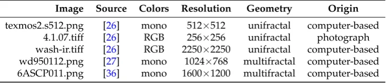
Multidimensional image analysis based on calculation of Γ(αi), Hα, and Ξα was tested on 5 standard 8-bpc images (Table 1). Before the computations, original images wd950112.gif and 6ASCP011.gif obtained from [27] were transformed into monochrome *.png formats in Matlabr software. All images were processed using an Image Info Extractor Professional software (Institute of Complex System, FFPW, USB, Czech Republic) forα={0.1, 0.2, ..., 0.9, 0.99, 1.1, 1.2, ..., 4.0}. The global information was extracted using (the italics refer to parameters which are set in the Image Info Extractor Professional software.) Whole Imagecalculation. The vertical-horizontal cross, square (a side of 5, 11, 15, and 29 px, respectively), and circle (a radius of 2, 5, and 8 px, respectively) local information was set as special cases of aCross,Rectangle, andEllipsecalculation at the rotation angle Phiof 0◦. Into the Image Info Extractor Professional software, a side of the square and radius of the circle surroundings is inputed aswidth/2 andheight/2 of 2, 5, and 14 px andaandbof 2, 5, and 8 px, respectively.

Table 1.Specifications of images.

Image Source Colors Resolution Geometry Origin

texmos2.s512.png [26] mono 512×512 unifractal computer-based 4.1.07.tiff [26] RGB 256×256 unifractal photograph wash-ir.tiff [26] RGB 2250×2250 unifractal computer-based wd950112.png [27] mono 1024×768 multifractal computer-based 6ASCP011.png [36] mono 1600×1200 multifractal computer-based

5.2. Calculation Algorithms

The algorithms implemented into the Image Info Extractor Professional are described in Algorithms1–2. In case of RGB images, the algorithms were applied to each color channel. The valuesΓ(αi)were visualized by a full rescaling into 8-bit resolution. Let us note that, forα= 1, the equations in lines 9 of both algorithms switch to the calculation of the Shannon entropy.

Acknowledgments: This work was supported by the Ministry of Education, Youth and Sports of the Czech Republic—projects CENAKVA (No. CZ.1.05/2.1.00/01.0024), CENAKVA II (No. LO1205 under the NPU I program), and The CENAKVA Centre Development (No. CZ.1.05/2.1.00/19.0380). JK acknowledges the support from the Czech Science Foundation, Grant No. GA14-07983S.

Author Contributions:Renata Rychtáriková is the main author of the text and tested the algorithms; Jan Korbel is responsible for the theoretical part of the article; Petr Macháˇcek and Petr Císaˇr are developers of the Image Info Extractor Professional software; Jan Urban is the first who derived the point information gain from the Shannon entropy; Dalibor Štys is the group leader who derived the point information gain for the Rényi entropy and prepared the first version of the manuscript. All authors have read and approved the final manuscript.

Conflicts of Interest:The authors declare no conflict of interest.

Appendix

All processed data are availableat [37] (for more details, see Section5):

2. Folder “H_Xi” stores the PIE_PIED.xlsx and PIE_PIED2.xlsx files with dependencies ofHα and

Ξα onαas exported from the PIE.mat files (in folder “Figures”). Titles of the graphs, which are in agreement with the computed variables and extracted kinds of information, are written in the sheets.

3. Folder “Histograms” stores the histograms of the occurrences of Γ(αi) values for the Cauchy (2 types), Lévy (3 types), and Gauss (4 types) distributions. The parameters of the original distributions are saved in the equation.txt files. All histograms were recalculated using 13 valuesα.

4. Folder “Software” contains a 32- and 64-bit version of an Image Info Extractor Professional v. b9 software (ImageExtractor_b9_xxbit.zip; supported by OS Win7) and a pig_histograms.m Matlabr script for recalculation of the typical probability density functions. A script pie_ec.m serves for the extraction ofHαandΞαfrom the folders (outputs from the Image Info Extractor Professional) overα. In the software and script, the variablesΓ(_αi),Hα, andΞαare calledPIG,PIE, andPIED, respectively. Manuals for the software and scripts are also attached.

References

1. Štys, D.; Urban, J.; Vanˇek, J.; Císaˇr, P. Analysis of biological time-lapse microscopic experiment from the point of view of the information theory. Micron2010,42, 3360–365.

2. Urban, J.; Vanˇek, J.; Štys, D. Preprocessing of microscopy images via Shannon’s entropy. Proceedings of Pattern Recognition and Information Processing, Minsk, Belarus, 2009, pp. 183–187.

3. Boer, P.T.D.; Kroese, D.; Mannor, S.; Rubinstein, R. A tutorial on the cross-entropy method. Ann. Oper. Res.

2002,134.

4. Baez, J.C.; Fritz, T.; Leinster, T. A characterization of entropy in terms of information loss. Entropy2011, 13, 1945–1957.

5. Marcolli, M.; Tedeschi, N. Entropy algebras and Birkhoff factorization. J. Geometry Phys.2015,97, 243–265. 6. Tsallis, C. Possible generalization of Boltzmann-Gibbs statistics. J. Stat. Phys.1988,52, 479–487.

7. Jizba, P.; Arimitsu, T. The world according to Rényi: Thermodynamics of multifractal systems. Ann. Phys.

2004,312, 17–59.

8. Jizba, P.; Korbel, J. Multifractal diffusion entropy analysis: Optimal bin width of probability histograms. Phys. A2014,413, 438–458.

9. Hentschel, H.; Procaccia, I. The infinite number of generalized dimensions of fractals and strange attractors. Phys. D1985,88, 435–444.

10. Campbel, L.L. A coding theorem and Rényi’s entropy. Inform. Control1965,8, 423–429.

11. Štys, D.; Jizba, P.; Papáˇcek, S.; Náhlik, T.; Císaˇr, P. On measurement of internal variables of complex self-organized systems and their relation to multifractal spectra. IWSOS 2012; F.A. Kuipers, P.H., Ed. Springer-Verlag, Berlin and Heidelberg, 2012, pp. 36–47.

12. Rényi, A. On measures of entropy and information. Proc. Fourth Berkeley Symp. on Math. Statist. and Prob.

1961,1, 547–561.

13. Kullback, S.; Leibler, R. On information and sufficiency.Ann. Math. Stat.1951,22, 79–86.

14. Csiszár, I. I-divergence geometry of probability distributions and minimization problems. Ann. Prob.1975, 3, 146–158.

15. Harremoes, P. Interpretations of Rényi entropies and divergences.Phys. Stat. Mech. Appl.2006,365, 5–62. 16. van Erven, T.; Harremoes, P. Rényi divergence and Kullback-Leibler divergence. IEEE Trans. Inf. Theory

2014,60, 3797–3820.

17. van Erven, T.; Harremoës, P. Rényi divergence and majorization. Information Theory Proceedings (ISIT), 2010 IEEE International Symposium on Information Theory. IEEE, 2010, pp. 1335–1339.

18. Jizba, P.; Kleinert, H.; Shefaat, M. Rényi’s information transfer between financial time series. Phys. A2012, 391, 2971–2989.

19. Havrda, J.; Charvát, F. Quantification method of classification processes. Concept of structuralα-entropy. Kybernetika1967,3, 30–35.

21. Grassberger, P.; Procaccia, I. Characterization of strange attractors. Phys. Rev. Lett.1983,50, 346–349. 22. Costa, M.H. A new entropy power inequality. IEEE Trans. Inform. Theory1985,31, 751–760.

23. Jizba, P.; Dunningham, J.A.; Joo, J. Role of information theoretic uncertainty relations in quantum theory. Ann. Phys.2015,355, 87–115.

24. Shannon, C.E. A mathematical theory of communication. Bell Syst. Tech. J.1948,27, 379–423. 25. Jizba, P.; Arimitsu, T. On observability of Rényi’s entropy. Phys. Rev. E2004,69, 026128. 26. http://sipi.usc.edu/database/database.php?volume=textures&image=61#top. 27. https://www.pinterest.com/pin/254031235202385248/.

28. Shalizi, C.R.; Crutchfield, J.P. Computational mechanics: Pattern and prediction, structure and simplicity. J. Stat. Phys.2011,104, 817–879.

29. Shalizi, C.R.; Shalizi, K.L. Quantifying self-organization in cyclic cellular automata. SPIE’s First International Symposium on Fluctuations and Noise. International Society for Optics and Photonics, 2003. 30. Shalizi, C.R.; Shalizi, K.L.; Haslinger, R. Quantifying self-organization with optimal predictors. Phys. Rev.

Lett.2004,93, 118701.

31. Crutchfield, J.P. Between order and chaos. Nat. Phys.2012,8, 17–24.

32. Zhyrova, A.; Štys, D.; Císaˇr, P. Macroscopic description of complex self-organizing system: Belousov-Zhabotinsky reaction. ISCS 2013; et al., A.S., Ed. Springer-Verlag, Berlin Heidelberg, Germany, 2014, Vol. 8,Emergence, Complexity and Computation, pp. 109–115.

33. Rychtarikova, R. Clustering of multi-image sets using Rényi information entropy. IWBBIO 2016; Ortuno.; Rojas., Eds. Springer, Switzerland, 2016, Vol. 9656,Lecture Notes in Computer Science, pp. 517–526.

34. Štys, D.; Urban, J.; Vanˇek, J.; Císaˇr, P. Analysis of biological time-lapse microscopic experiment from the point of view of system theory. Micron2011,7, 360–365.

35. Štys, D.; Vanˇek, J.; Náhlík, T.; Urban, J.; Císaˇr, P. The cell monolayer trajectory from the system state point of view. Mol. BioSyst.2011,42, 2824–2833.

36. http://cims.nyu.edu/ kiryl/Photos/Fractals1/ascp011et.html. 37. ftp://160.217.215.251/pig (user: anonymous; password: anonymous).

c