Competitive Analysis of Task Scheduling Algorithms on a Fault-Prone Machine
and the Impact of Resource Augmentation
Antonio Fern´andez Antaa, Chryssis Georgioub, Dariusz R. Kowalskic, Elli Zavoua,d,1 aInstitute IMDEA Networks
bUniversity of Cyprus cUniversity of Liverpool dUniversidad Carlos III de Madrid
Abstract
Reliable task execution in machines that are prone to unpredictable crashes and restarts is challenging and of high importance. However, not much work exists on the worst case analysis of such systems. In this paper, we analyze the fault-tolerant properties of four popular scheduling algorithms: Longest In System (LIS), Shortest In System (SIS), Largest Processing Time (LPT) and Shortest Processing Time (SPT), under worst case scenarios on a fault-prone machine. We use three metrics for the evaluation and comparison of their competitive performance, namely, completed time, pending time and latency. We also investigate the effect of resource augmentation in their performance, by increasing the speed of the machine. To do so, we compare the behavior of the algorithms for different speed intervals and show that between LIS, SIS and SPT there is no clear winner with respect to all the three considered metrics, while LPT is not better than SPT.
Keywords: Scheduling, Online Algorithms, Different Task Processing Times, Failures, Competitive Analysis, Resource Augmentation
1. Introduction
Motivation. The demand for processing computationally-intensive jobs has been increasing dramatically during the last decades, and so has the research to face the many challenges it presents. In addition, with the presence of machine failures (and restarts) things get even worse, especially when a malicious entity is causing them. In this work, we applyspeed augmentation[9, 1] in order to overcome such failures, that is, we increase the computational power of the system’s machine. This is an alternative to increasing the number of processing entities, as done in multiprocessor systems. Hence, we consider a speedups≥1, under which the machine performs a jobstimes faster than the baseline execution time.
More precisely, we consider a setting with a singlemachineprone to crashes and restarts that are being controlled by an adversary, and a schedulerthat assigns injected jobs (or tasks) to be executed by the machine. These tasks arrive continuously and have different computational demands and hence processing time. Specifically we assume that each task has processing time π ∈ [πmin, πmax], where πmin andπmax are the smallest and largest values,
respectively. Since the scheduling decisions must be made continuously and without knowledge of the future, neither the task injections nor the machine crashes and restarts, we look at the problem as anonlinescheduling problem [10, 4, 3, 12, 14]. The importance of using speedup lies on this online nature of the problem; the future failures, and the
instant of arrival of future new tasks and their processing time are unpredictable. Thus, the need to overcome this lack of information. We evaluate the performance of the different scheduling policies (online algorithms) under worst-casescenarios, which guarantee efficient scheduling even in the worst of cases. For that, we perform competitive analysis [13]. The four scheduling policies we consider areLongest In System(LIS),Shortest In System(SIS),Largest Processing Time(LPT) andShortest Processing Time(SPT). Achieving reliable and stable computations in such an environment withholds several challenges. One of our main goals is therefore to confront these challenges considering the use of the smallest possible speedup. However, our primary intention is to discover the dependence of the efficiency measures for each scheduling policy with respect to the speedup used.
Contributions. In this paper we explore the behavior of some of the most widely used algorithms in scheduling, analyzing their fault-tolerant properties under worst-case combination of task injection and crash/restart patterns, as described above. As already mentioned, the four algorithms we consider are:
(1) LIS: the task that has been waiting the longest is scheduled; i.e., it follows the FIFO(First In First Out)policy, (2) SIS: the task that has been injected the latest is scheduled; i.e., it follows the LIFO(Last In First Out)policy, (3) LPT: the task with the longest processing time is scheduled, and
(4) SPT: the task with the shortest processing time is scheduled.
We focus on threeevaluation metrics, which we regard to embody the most important quality of service parame-ters: thecompleted time,which is the aggregate processing time of all the tasks that have completed their execution successfully, thepending time,which is the aggregate processing time of all the tasks that are in the queue waiting to be completed, and thelatency,which is the largest time a task spends in the system, from the time of its arrival until it is fully executed. They represent the machine’s throughput, queue size and delay respectively, all of which we consider essential. They show how efficient the scheduling algorithms are in a fault-prone setting from different angles: machine utilization (completed time), buffering (pending time) and fairness (latency). The performance of an algorithm ALG is evaluated under these three metrics by means of competitive analysis, in which the value of the metric achieved by ALG when the machine uses speedups ≥ 1 is compared with the best value achieved by any algorithmXrunning without speedup (s= 1) under the same pattern of task arrivals and machine failures, at all time instants of an execution.
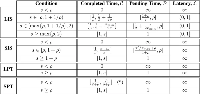
Table 1 summarizes the results we have obtained for the four algorithms. Although not clearly stated in the table, the first results we show in our work apply toany work conserving scheduling algorithm– ones that do not idle as long as there are pending tasks and they do not break the execution of a task unless the machine crashes. These results are: (a) Whens ≥ρ= πmax
πmin, the completed time competitive ratio is lower bounded by1/ρand the pending time
competitive ratio is upper bounded byρ. (b) Whens≥1 +ρ, the completed time competitive ratio is lower bounded by1and the pending time competitive ratio is upper bounded by1(i.e., they are 1-competitive). Then, for specific cases of speedup less than1 +ρwe obtain better lower and upper bounds for the different algorithms.
However, it is clear that none of the algorithms is better than the rest. With the exception of SPT, no algorithm is competitive in any of the three metrics considered whens < ρ. In particular, algorithm SPT is competitive in terms of completed time, except in the case when tasks may have any arbitrary processing time in the range[πmin, πmax]and
the machine has no speedup (s= 1). In terms of latency, only algorithm LIS is competitive, whens≥ρ, which might not be very surprising since algorithm LIS gives priority to the tasks that have been waiting the longest in the system. Another interesting observation is that algorithms LPT and SPT become 1-competitive as soon ass≥ρ, both in terms of completed and pending time, whereas LIS and SIS require greater speedup to achieve this.
Condition Completed Time,C Pending Time,P Latency,L
LIS
s < ρ 0 ∞ ∞
s∈[ρ,1 + 1/ρ) [ρ1,12+21ρ] [1+2ρ, ρ] (0,1]
s∈[max{ρ,1 + 1/ρ},2) [1ρ,12+πmin
2π ] [
1 2+
π
2πmin, ρ] (0,1]
s≥max{ρ,2} [1, s] 1 (0,1]
SIS
s < ρ 0 ∞ ∞
s∈[ρ,1 +ρ) [1ρ,πmin
π0 ] [
π0/πmin+ρ
1+ρ , ρ] ∞
s≥1 +ρ [1, s] 1 ∞
LPT s < ρ 0 ∞ ∞
s≥ρ [1, s] 1 ∞
SPT s < ρ [
1 2+ρ,
ˆ ρ ˆ
ρ+ρ] (*) ∞ ∞
s≥ρ [1, s] 1 ∞
Table 1: Metrics comparison of the four scheduling algorithms. Recall thatsrepresents the speedup of the system’s machine, πmax andπminthe largest and smallest task processing times respectively. Note thatρ = ππmax
min, ρˆ = dρe −1andπ, π
0 ∈
(πmin, πmax)are task processing times such thatπ < πsmin−1 andπ0<πmin+sπmax. Note also that by definition,0-completed-time
competitiveness ratio equals to non-competitiveness, as opposed to the other two metrics where non-competitiveness corresponds to an∞competitiveness ratio. Finally note that the lower bound of result (*) is for injection patterns with tasks of only two processing timesπminandπmax.
that give priority based on the requiredprocessing timeof the tasks (LPT and SPT). Observe that different algorithms scale differently with respect to the speedup, in the sense that with the increase of the machine speed the competitive performance of each algorithm changes in a different way.
Related Work. We relate our work with the online version of thebin packingproblem [15], where the objects to be packed are the tasks and the bins are the time periods between two consecutive failures of the machine (i.e.,alive intervals). Wide research has taken place over the years around this problem, some of which we consider related to ours. For example, Johnson et al. [8] analyzed the worst case performance of two simple algorithms (Best Fit and Next Fit) for the bin packing problem, giving upper bounds on the number of bins needed (corresponding to the completed time in our work). Epstein et al. [6] (see also [15]) considered online bin packing with resource augmentation in the size of the bins (corresponding to the length of alive intervals in our work). Observe that the essential difference of the online bin packing problem with the one that we are looking at in this work, is that in our system the bins and their sizes (corresponding to the machine’s alive intervals) are unknown.
On a different tone, Boyar and Ellen [5] have looked into a problem similar to both online bin packing problem and ours, considering job scheduling in the grid. The main difference with our setting is that they consider several machines (or processors), but mainly the fact that the arriving items are processors with limited memory capacities and there is a fixed amount of jobs in the system that must be completed. They also use fixed job sizes and achieve lower and upper bounds that only depend on the fraction of such jobs in the system.
Another related problem is packet scheduling in a link. Andrews and Zhang [2] consider online packet scheduling over a wireless channel whose rate varies dynamically, and perform worst case analysis regarding both the channel conditions and the packet arrivals. A similar work is [3], where packets of two different sizes were scheduled through an unreliable link. In that work, the goodness metric is the long-term competitive ratio, which is called relative throughputand online algorithms as well as bounds for any online scheduling protocol are given.
unex-pected machine breakdowns. However, in most related works preemptive scheduling is considered and optimality is shown only for nearly online algorithms (need to know the time of the next job or machine availability).
In a previous work [4], we looked at a system of multiple machines and at least two different task costs (i.e., processing times in our work). We applied distributed scheduling and performed worst-case competitive analysis, considering the pending cost competitiveness (corresponding pending time competitiveness in the present work) as our main evaluation metric. We showed the NP-hardness of the offline version of the problem and suggested the use ofspeedupin order to achieve competitiveness. We definedρ= πmax
πmin and proved that if both conditions (a)s < ρ
and (b) s < 1 +γ/ρhold for the system’s machines (γ is some constant that depends on πmin andπmax), then
nodeterministic algorithm is competitive with respect to the queue size (pending cost). Additionally, we proposed online algorithms to show that relaxing any of the two conditions is sufficient to achieve competitiveness. In fact, [4] motivated this paper, since it made evident the need of a thorough study of simple algorithms even under the simplest basic model of one machine and scheduler.
2. Model and Definitions
Computing Setting.We consider a system of one machine prone to crashes and restarts with aSchedulerresponsible for the task assignment to the machine following some algorithm. The clients submit jobs (ortasks) of different sizes (processing time) to the scheduler, which in its turn assigns them to be executed by the machine.
Tasks.Tasks are injected to the scheduler by the clients of the system, an operation which is controlled by an arrival pattern A(a sequence of task injections). Each taskτ has an arrival timea(τ)and aprocessing timeπ(τ), being the time it requires to be completed by a machine running withs = 1. We use the termπ-task to refer to a task of processing timeπ ∈[πmin, πmax]throughout the paper. We also assume tasks to beatomicwith respect to their
completion; in other words preemption is not allowed (tasks must be fully executed without interruptions).
Machine failures. The crashes and restarts of the machine are controlled by an error patternE, which we assume to coordinate with the arrival pattern in order to give the worst-case scenarios. We consider that the task being executed at the time of the machine’s failure is not completed, and it is therefore still pending in the scheduler until it is eventually re-scheduled (it is not discarded). The machine isactivein the time interval[t, t∗], if it is executing some task at timet and has not crashed by timet∗. Hence, an error patternEcan be seen as a sequence of active intervals of the machine. Resource augmentation / Speedup.We also consider a form of resource augmentation by speeding up the machine and the goal is to keep it as low as possible. As mentioned earlier, we denote the speedup withs≥1.
Notation.Let us denote here some notation that will be extensively used throughout the paper. Because it is essential to clarify the tasks being accounted at each timepoint in an execution, we introduce setsIt(A), Nts(X, A, E)and
Qs
t(X, A, E), whereX is an algorithm,A andE the arrival and error patterns respectively, t the time instant we
are looking at andsthe speedup of the machine. It(A)represents the set of injected tasks within the interval[0, t],
Ns
t(X, A, E) the set of completed tasks within [0, t] and Qst(X, A, E)the set of pending tasks at time instant t.
Qs
t(X, A, E)contains the tasks that were injected by timetinclusively, but not the ones completed before and up to
timet. Observe thatIt(A) = Nts(X, A, E)∪Qst(X, A, E)and note that setIdepends only on the arrival pattern
A, while setsN andQalso depend on the error patternE, the algorithm run by the scheduler,X, and the speedup of the machine,s. Note that the supersciptsis omitted in further sections of the paper for simplicity. However, the appropriate speedup in each case is clearly stated.
Cts(ALG, A, E) = X
τ∈Ns
t(ALG,A,E)
π(τ),
thePending Time, which is the sum of processing times of the pending tasks Pts(ALG, A, E) = X
τ∈Qs
t(ALG,A,E)
π(τ),
and theLatency, which is the maximum amount of time a task has spent in the system
Lst(ALG, A, E) = max
(
f(τ)−a(τ), ∀τ ∈Nts(ALG, A, E)
t−a(τ), ∀τ ∈Qs
t(ALG, A, E) )
,
wheref(τ) is the time of completion of taskτ. Computing the schedule (and hence finding the algorithm) that minimizes or maximizes correspondingly the measuresCs
t(X, A, E), Pts(X, A, E),andLst(X, A, E)offline (having
the knowledge of the patternsAandE), is an NP-hard problem [4].
Due to the dynamicity of the task arrivals and machine failures, we view the scheduling of tasks as an online problem and pursuecompetitive analysis using the three metrics. Note that for each metric, we consider any time tof an execution, combinations of arrival and error patterns AandE, and any algorithm X designed to solve the scheduling problem:
An algorithm ALG running with speedup s, is consideredα-completed-time-competitive ifCs
t(ALG, A, E) ≥
α·C1
t(X, A, E) + ∆C, for some parameter∆C that does notdepend on t, X, Aor E; α is the completed-time
competitive ratio of ALG, which we denote byC(ALG). Similarly, it is consideredα-pending-time-competitiveifPs
t(ALG, A, E)≤α·Pt1(X, A, E) + ∆P, for parameter
∆P which does not depend ont, X, AorE. In this case,αis the pending-time competitive ratio of ALG, which we
denote byP(ALG).
It is also consideredα-latency-competitiveifLs
t(ALG, A, E)≤α·L1t(X, A, E) + ∆L, where∆Lis a parameter
independent oft, X, AandE. In this case,αis the latency competitive ratio of ALG, which we denote byL(ALG). Finally, note thatα, is independent oft,X,AandE, for the three metrics accordingly.2
Both completed and pending time measures are important. Observe that they are not complementary of one another. An algorithm may be completed-time-competitive but not pending-time-competitive, even though the sum of processing times of the successfully completed tasks complements the sum of processing times of the pending ones. For example, think of an online algorithm that manages to complete successfully half of the total injected task processing times up to any point in any execution. This gives a completed time competitiveness ratioC(ALG) = 1/2. However, it is not necessarily pending-time-competitive since in an execution with infinite task arrivals its total pending time increases unboundedly and there might exist an algorithmXthat manages to keep its total pending time constant under the same arrival and error patterns. This is further demonstrated by our results summarized in Table 1.
3. Properties of Work Conserving Algorithms
In this section we present some general properties for all online work-conserving algorithms running with speedups. They also apply to the four policies we focus on in the rest of the paper.
Observation 1. Any work-conserving algorithm ALG running with speedups, has a completed-time competitive ratio
C(ALG)≤1when we allowQt(ALG) =∅infinitely many times, orC(ALG)≤swhen the queue never becomes empty
after a point in time.
2Parameters∆
C,∆P,∆Las well asαmay depend on system parameters likeπmin,πmaxors, which are not considered as inputs of the
Proof: Let us first consider the case at which the adversary allows the queue of pending tasks of ALG to become empty infinitely many times in an execution. In particular, let us consider the arrival and error patternsAandE, such that there are time instantstk, k= 0,1,2. . . wheretk =tk−1+πandt0= 0. At eachtkthere is a machine failure
(crash and restart) and exactly oneπ-task (π∈[πmin, πmax]) injected. We name time intervalTi= [ti, ti+1]. Observe
that an algorithmX (running withs = 1) completesπ-task injected attiin intervalTi, while any work-conserving
algorithm ALG running with speedupswill complete the same task at timeti+π/s < ti+1 resulting in an empty
queue. Hence,C(ALG) = 1as claimed.
Let us now consider the case at which the adversary never lets the queue of ALG to become empty after some point in time. More precisely we consider the arrival and error patternsA0 andE0 to be such that ALG always has at least one pending task of any processing timeπ∈ [πmin, πmax]available to schedule. Therefore, in a period of
timeπan algorithmX ∈ X (running withs = 1) is able to complete aπ-task while ALG may complete up toπs processing time. This will result in a completed time competitive ratioC(ALG)≤sas claimed.
Observation 2. Any work-conserving algorithm ALG running with speedups, has a pending-time competitive ratio
P(ALG)≥1when its queue of pending tasks never becomes empty after a point in time.
Proof: Let us consider arrival and error patternsAandEsuch that algorithm ALG always has at least one pending task of any processing timeπ∈[πmin, πmax]available to schedule. We consider phases of arbitrarily chosen lengths
π, defined as intervalsTi = [tk, tk+1]wheretk+1 =tk+π,t0 = 0andk = 0,1,2. . . being instants of machine
failures. As a result, in a phase of lengthπan algorithmX ∈ X will be able to complete aπ-task, while ALG will complete up toπsprocessing time. Assuming that there are no phases of length less thanπmin, the complementing
pending time at a timetkwill therefore bePtk(X)≥Itk(A)−tk andPtk(ALG)≥Itk(A)−tks. The pending time
competitive ratio becomesP(ALG) ≥ II((AA))−−tst, which yields toP(ALG) ≥ 1, since we can makeI(A)infinitely big.
Lemma 1. No algorithmX (running without speedup) completes more tasks than a work conserving algorithm ALG running with speedup s ≥ ρ. Formally, ∀t, A ∈ A and E ∈ E, |Nt(ALG, A, E)| ≥ |Nt(X, A, E)|, and hence |Qt(ALG, A, E)| ≤ |Qt(X, A, E)|.
Proof: We will prove that ∀t, A ∈ A and E ∈ E, |Qt(ALG, A, E)| ≤ |Qt(X, A, E)|, which implies that |Nt(ALG, A, E)| ≥ |Nt(X, A, E)|. Observe that the claim trivially holds for t = 0. We now use induction on
t to prove the general case. Consider any time t > 0 and the closest time t0 < t such that t0 is either a fail-ure/restart time point or a point where ALG’s pending queue is empty. Let us assume by induction hypothesis that
|Qt0(ALG)| ≤ |Qt0(X)|.
LetiT be the number of tasks injected in the intervalT = (t0, t]. Since ALG is work conserving, it is continuously
executing tasks in the intervalT. Also, ALG needs at mostπmax/s≤πmintime to execute any task using speedup
s≥ρ, regardless of the task being executed. Then it holds that
|Qt(ALG)| ≤ |Qt0(ALG)|+iT −
t−t0
πmax/s
≤ |Qt0(ALG)|+iT −
t−t0
πmin
.
On the other hand,X can complete at most one task everyπmintime. Hence, |Qt(X)| ≥ |Qt0(X)|+iT−
t−t0
πmin
.
|Qt(X)| − |Qt(ALG)| ≥ |Qt0(X)|+iT−
t−t0
πmin
− |Qt0(ALG)| −iT +
t−t0
πmin
≥0.
Since this holds for all timest, the claim follows.
Theorem 1. Any work-conserving algorithm ALG running with speedups≥ρhas completed-time competitive ratio
C(ALG)≥1/ρand pending-time competitive ratioP(ALG)≤ ρ.
Proof: It follows directly from Lemma 1, since for any algorithmX the processing time of every task completed by ALG is at least πmin
πmax times the processing time of every task completed byX. From Lemma 1, ALG always has at
least as many completed tasks asX, and hence its completed-time competitive ratioC(ALG)is at least πmin
πmax = 1/ρ.
Complementary, since the processing time of any pending task in the queue of ALG is at most πmax
πmin times bigger than
the processing time of any pending task inX, its pending-time competitive ratioP(ALG)is at most πmax
πmin =ρ.
Theorem 2. Any work-conserving algorithm ALG running with speedups≥1 +ρ, has completed-time competitive ratioC(ALG)≥1and pending-time competitive ratioP(ALG)≤ 1.
Proof: Consider an execution of any work-conserving algorithm ALG running with speedups ≥ 1 +ρunder any arrival and error patternsAandE, as well as an algorithmX. Then, looking at any timetof an execution, we define time instantt0 < tto be the latest time beforetat which one of the following events happens: (1) anactive period starts (after a machine crash/restart), (2) algorithmX has successfully completed a task, or (3) the queue of pending tasks of ALG is empty,Qt0(ALG) =∅.
It is trivial that P0(ALG, A, E) ≤ P0(X, A, E)holds at the beginning of the executions. Now assuming that Pt0(ALG, A, E) ≤ Pt0(X, A, E)holds at timet0, we prove by induction that Pt(ALG, A, E) ≤ Pt(X, A, E)still
holds at timet. This also means that the tasks successfully completed by ALG by timethave at least the same total processing time as the ones completed byX.
Considering the intervalT = (t0, t], there are two cases:
Case 1: X is not able to complete any task in the interval T. Then, it holds thatPt(X, A, E) = Pt0(X, A, E) +
iT, where iT denotes the processing time of the tasks injected during the interval T. Similarly, it holds that
Pt(ALG, A, E)≤Pt0(ALG, A, E) +iT even if ALG is not able to complete successfully any task inT.
Case 2:X completes successfully a task in the intervalT. Note that by definition of timet0, during intervalT there can only be one task completed byX, and it must be completed at timet. (If that were not the case,t0would not be well defined.) There are two subcases.
(a) First,t0is from case (3) of its definition. Hence,Qt0(ALG) =∅andPt(ALG, A, E)≤iT. At timet0algorithmX
was executing the task that was completed at timet. Hence, the task was injected beforet0, andXhas not completed any of the tasks injected inT. Then,Pt(X, A, E)≥iT ≥Pt(ALG, A, E).
(b) Second, t0 is from cases (1) or (2) of its definition. Then, the intervalT has lengthπ ≥ πmin, which is the
processing time of the task completed by X. In that interval ALG is continuously executing tasks. Hence, in the interval (t0, t] if completes tasks whose aggregate processing time is at least πs−πmax. Then, the pending
time at time instantt of both algorithms satisfyPt(X, A, E) = Pt0(X, A, E) +iT −πwhile Pt(ALG, A, E) <
Pt0(ALG, A, E) +iT−(πs−πmax). Observe thats≥1 +ρimplies thatπ≤πs−πmax. Hence, from the induction
hypothesis,Pt(ALG, A, E)≤Pt(X, A, E).
4. Completed and Pending Time Competitiveness
In this section we present a detailed analysis of the four algorithms with respect to the completed and pending time metrics, first for speedups < ρand then for speedups≥ρ.
4.1. Speedups < ρ
Let us start with some negative results, whose proofs involve specifying the combinations of arrival and error patterns that force the claimedbadperformances of the algorithms. We also give some positive results for SPT, the only algorithm that can achieve a non-zero completed-time competitiveness under some cases.
Lemma 2. When algorithms LIS and LPT run with speedups < ρ, they both have a completed-time competitive ratio
C(LIS) =C(LPT) = 0and a pending-time competitive ratioP(LIS) =P(LPT) =∞.
Proof: Let us use the same combination of algorithmX, arrival and error patternsAandE for the proof of non-competitiveness for the two algorithms. We consider an infinite arrival pattern which injects oneπmax-task at the
beginning of the execution,t = 0, and after that it keeps injecting one πmin-task everyπmin time. Consider also
an infinite error pattern that sets the machine failure points (crash immediately followed by a restart) at time instants ti =i·πmin, wherei= 1,2, . . . .
It can be easily seen, that an algorithmXrunning with no speedup (s= 1), will be able to complete theπmin-tasks
injected, while neither LIS nor LPT will manage to complete any task, since they will both insist on scheduling the πmax-task injected at the beginning. In an interval of lengthπmin, algorithmX is able to complete aπmin-task but
neither LIS nor LPT can complete theπmax-task since it needs time πmaxs > πmin. This means that the number of
pending tasks in the queues of both LIS and LPT will be continuously increasing with time, whileX is able to keep them bounded, with no more than oneπmaxand oneπmintasks, and so will their pending processing time. As for the
total processing time of completed tasks,C(LIS, A, E) =C(LPT, A, E) = 0at all times of the execution, while the one ofX grows to infinite astgoes to infinity.
Hence, for speedups < ρ, algorithms LIS and LPT have completed-time competitive ratiosC(LIS) =C(LPT) = 0
and pending-time competitive ratiosP(LIS) =P(LPT) =∞as claimed, which completes the proof.
Lemma 3. When algorithm SIS runs with speedups < ρ, it has a completed-time competitive ratioC(SIS) = 0and a pending-time competitive ratioP(SIS) =∞.
Proof:Let us divide the proof in two parts giving different combinations of arrival and error patterns for the completed time and the pending time respectively.
We first consider a combination of arrival and error patternsA andE that behave as follows. We define time instantstkwherek= 1,2, . . . andti=ti−1+πminwith timet0= 0being the beginning of the execution. At every
such time instants there is a crash and restart at the machine and then an immediate injection of aπmin-task followed
by aπmax-task. This createsactiveintervals[ti, ti+1)of lengthπmin.
It is easy to observe that the patterns described cause algorithm SIS to assign the lastπmax-task injected, every
time it has to make a scheduling decision, since it is the last task injected. Since thealiveintervals are of lengthπmin
and SIS needs πmax
s > πmin time to complete theπmax-tasks, it is not able to complete any of the tasks it starts
executing, givingCt(SIS) = 0at all timest(and in particular attktime instants). On the same time, an algorithmX
is able to schedule and complete all theπmin-tasks injected, one in every alive interval, giving a completed time of
Now let us consider another combination of arrival and error patterns,A0andE0respectively as well as algorithm X0. We define time instantstk0 wherek0 = 1,2, . . . andtk0 = tk0−1+ (πmin +πmax)with timet0 = 0being
the beginning of the execution. At every such time instants there is aπmin-task injected followed by aπmax-task.
The crashes of the machine are set every timetk0 andtk0+πmin, creatingactiveintervals of lengthπmin orπmax
alternatively.
This behavior causes algorithm SIS to schedule the lastπmax-task injected, after everytk0time instant, since it is
the last task injected. The first alive interval after atk0 time instant is of lengthπminand thus theπmax-task scheduled
by SIS cannot be completed. On the same time, an algorithmXis able to complete the lastπmin-task injected. On the
next alive period though, SIS will be able to complete successfully theπmax-task since it is of lengthπmax, whileX
will do the same. As a result, looking at time instantstk0, before the injection takes place,Pt
k0(SIS) =k 0π
minwhile
Ptk0(X) = 0, since algorithm SIS will never complete anyπmin-task injected butXwill be able to complete all tasks
injected up to that time.
Therefore, for speedups < ρalgorithm SIS has completed-time competitive ratioC(SIS) = 0and pending-time competitive ratioP(SIS) =∞as claimed.
Combining now Lemmas 2 and 3 we have the following theorem.
Theorem 3. NONE of the three algorithms LIS, LPT and SIS is competitive when speedups < ρ, with respect to completed or pending time, even in the case of only two task processing times (i.e.,πminandπmax).
Theorem 4. If tasks can be of only two processing times (πminandπmax), algorithm SPT can achieve a
completed-time competitive ratioC(SPT)≥ 1
2+ρ, for any speedups≥1. In particular,Ct(SPT)≥ 1
2+ρCt(X)−πmax, for any
timet.
Proof:Let us assume fixed arrival and error patternsAandErespectively, as well as an algorithmX, and let us look at any timetin the execution of SPT. Letτ be a task completed byX by timet(i.e.,τ ∈Nt(X)), wheretτ is the
timeτ was scheduled andf(τ)≤ tthe time it completed its execution. We associateτ with the following tasks in Nt(SPT):
• The same taskτ.
• The taskwbeing executed by SPT at timetτ, if it was not later interrupted by a crash.
Not every task inNt(X)is associated to some task inNt(SPT), but we show now that most tasks are. In fact, we show
that the aggregate processing times of the tasks inNt(X)that are not associated with any task inNt(SPT)is at most
πmax. More specifically, there is only one task execution of aπmax-task, namelyw, by SPT such that theπmin-tasks
scheduled and completed byX concurrently with the execution ofwfall in this class. Considering the generic taskτ∈Nt(X)from above, we consider the following cases:
• Ifτ∈Nt(SPT)then taskτis associated at least with itself in the execution of SPT, regardless ofτ’s processing
time.
• Ifτ /∈Nt(SPT),τis in the queue of SPT at timetτ. By its greedy nature, SPT is executing some taskwat time
tτ.
– Ifπ(τ)≥π(w), then taskwwill complete by timef(τ)and hence it is associated withτ.
– Ifπ(τ) < π(w)(i.e.,π(τ) = πmin andπ(w) = πmax), thenτ was injected afterwwas scheduled by
Lett∗the time either event occurs. Sinceτ /∈Nt(SPT),τis not completed by SPT in the interval[t∗, t].
Then, SPT never schedules aπmax-task in the interval[t∗, t], and the case that a task fromNt(X)is not
associated to any task inNt(SPT)cannot occur again in that interval.
Hence, all the tasksτ ∈Nt(X)that are not associated to tasks inNt(SPT)areπmin-tasks and have been scheduled
and completed during the execution of the sameπmax-task by SPT. Hence, their aggregate processing time is at most
πmax.
Now let us evaluate the processing times of the tasks inNt(X)associated to a task inw ∈ Nt(SPT). Let us
consider any taskwsuccessfully completed by SPT at a timef(w)≤t. Taskwcan be associated at most with itself and all the tasks thatX scheduled within the intervalTw = [f(w)−π(w), f(w)]. The latter set can include tasks
whose aggregate processing time is at mostπ(w) +πmax, since the first such tasks starts its execution no earlier
thanf(w)−π(w)and in the extreme case aπmax-task could have been scheduled af the end ofTwand completed at
tw+πmax. Hence, if taskwis aπmin-task, it will be associated with tasks completed byXthat have a total processing
time of at most2πmin+πmax, and ifwis aπmax-task, it will be associated with tasks completed byX that have a
total processing time of at most3πmax. Observe that 2πminπmin+πmax < 3ππmaxmax. As a result, we can conclude that
Ct(SPT)≥
πmin
2πmin+πmax
Ct(X)−πmax=
1
2 +ρCt(X)−πmax.
Conjecture 1. The above lower bound on completed time, still holds in the case of any constant number of task processing times in the range[πmin, πmax].
Theorem 5. For speedup s < ρ, algorithm SPT cannot have a completed-time competitive ratio more than xfor x < ρˆ+ρˆρ. In other words,C(SPT)≤ ρˆ+ρˆρ. Additionally, it is NOT competitive with respect to the pending time, i.e.,
P(SPT) =∞.
Proof: Assuming speedup s < ρwe consider the following combination of arrival and error patterns A andE respectively: We define time pointstk, where k = 0,1,2. . ., such thatt0 is the beginning of the execution and tk =tk−1+πmax+ ˆρπmin(recall thatρˆ=dρe −1 < ρ). At everytk time instant there areρˆtasks of processing
timeπmininjected along with oneπmax-task. What is more, the crash and restarts of the system’s machine are set at
timestk+πmaxand then after everyπmintime untiltk+1is reached.
By the arrival and error patterns described, every epoch; time interval [tk, tk+1], results in the same behavior.
Algorithm SPT is able to complete only theρˆtasks of processing timeπmin, whileX is able to complete all tasks
that have been injected at the beginning of the epoch. From the nature of SPT, it schedules first the smallest tasks, and therefore theπmaxones never have the time to be executed; aπmax-task is scheduled at the last phase of each epoch
which is of sizeπmin(recalls < ρ⇒s <ρˆ). Hence, at timetk,Ctk(SPT, A, E) =kρπˆ minandCtk(X, A, E) =
kρπˆ min+kπmax.
Looking at the pending time at such points, we can easily see that SPT’s is constantly increasing, whileXis able to have pending time zero;Ptk(SPT, A, E) =kπmaxbutPtk(X, A, E) = 0.
As a result, we have a maximum completed-time competitive ratio C(SPT) ≤ kρπˆ min
kρπˆ min+kπmax =
ˆ ρ ˆ
ρ+ρ and a
pending timeP(SPT) =∞.
Theorem 6. If tasks can have any processing time in the range [πmin, πmax], and there is no speedup (s = 1),
Proof: Assumings = 1, we consider the following scenario as a result of adversarial arrival and error patternsA andE respectively. Let us fix some ∈ (0,1)and use the notation∆(k) = (πmax−πmin)k. Then, letwk be a
task with processing timeπ(wk) =πmin+ ∆(k), for allk= 0,1,2,3, . . .. Observe that∀k, π(wk)∈(πmin, πmax]
andπ(wk+1) < π(wk). Let us also define time pointstk, such thatt0 = 0(the beginning of the execution) and tk+1 =tk+πmin+1+2∆(k). Let us also define time pointst0k =tk−1+ 1−2∆(k). The arrival patternAis such
that taskw0=πmaxis injected in the system at time instantt0. Then, fork= 1,2, . . .taskwkis injected at timet0k.
The error patternEis such that at every time instanttkthere is a crash and restart.
We compare SPT with an algorithmXof our choice. In the execution of SPT, taskw0is scheduled as soon as it
arrives, at timet0. On the other hand,Xwaits until timet01for the arrival ofw1and schedules it immediately. When
the processors crashes at timet1the taskw0 executed by SPT is interrupted, sincet1−t0 = πmin+ 1+2∆(0)<
π(w0) =πmin+ ∆(0). However,Xis able to complete taskw1becauset01+π(w1) = 1−2∆(1) +πmin+ ∆(1) =
πmin+1+2∆(0) =t1. After the restart att1SPT schedules taskw1, whileXwaits untilt02to schedulew2.
The general process is as follows. At time instanttk, SPT schedules taskwk whileX waits until taskwk+1 is
injected at timet0k+1 and schedules it. When the processors crashes at timetk+1 the taskwk of SPT is interrupted,
sincetk+1−tk =πmin+1+2∆(k)< π(wk) =πmin+ ∆(k). However,Xis able to complete taskwk+1because t0k+1+π(wk+1) = 1−2∆(k+ 1) +πmin+ ∆(k+ 1) =πmin+1+2∆(k) =tk+1.
Letting this adversarial behavior run to infinity we see that at any point in timet,Ct(SPT) = 0, whileXwill keep
completing the injected tasks. This, results to a completed-time competitive ratioC(SPT) = 0.
4.2. Speedups≥ρ
First, recall that in Theorem 1 we have shown that any work conserving algorithm running with speedups≥ρhas pending-time competitive ratio at mostρand completed-time competitive ratio at least1/ρ. So do the four algorithms LIS, LPT, SIS and SPT. A natural question that rises is whether we can improve these ratios. Let us start from some negative results again, focusing at first on the two policies that schedule tasks according to their arrival time, algorithms LIS and SIS.
Lemma 4. When algorithm LIS runs with speedups∈[ρ,1+1/ρ), it has a completed-time competitive ratioC(LIS)≤ 1
2+ 1
2ρand a pending-time competitive ratioP(LIS)≥ 1+ρ
2 .
Proof: Let speedups∈[ρ,1 + 1/ρ). We define a combination of arrival and error patternsAandE, and algorithm X. PatternsAandEbehave as follows: Initially, there is aπmin-task injected, followed by aπmax-task. After every
period ofπmaxtime the same injection sequence is repeated, when also the machine is crashed and restarted.
This behavior results to the following execution. There are only active phases of size πmax, during which
an algorithmX can successfully execute the πmax task injected, while LIS is forced to schedule the tasks in the
order they arrive. Observe that, sinces < 1 + 1/ρ = (πmin +πmax)/πmax, LIS is able to complete only one
task in each phase. Observe also, that afterkphases, wherekis an multiple of 2, there will be exactlyk tasks of sizeπmin pending in the queue ofX, while LIS will have pending half of the tasks injected, half of which are of
processing timeπminand the other halfπmax. Hence, the pending-time competitive ratio of the algorithm becomes P(LIS) = πmin+πmax
2πmin =
1+ρ
2 and the completed-time competitive ratioC(LIS) =
πmin+πmax
2πmax =
1 2 +
1 2ρ, which
completes the proof.
Lemma 5. When algorithm LIS runs with speedups∈[1+1/ρ,2), it has a completed-time competitive ratioC(LIS)≤ 1
2+ πmin
2π and a pending-time competitive ratioP(LIS)≥ 1 2+
π
2πmin for any processing timeπ∈(πmin, πmax)such
thatπ < πmin
Proof: Let speedups∈[1 + 1/ρ,2). We define a combination of arrival and error patternsAandE, and algorithm X to behave as follows: We define time instants tk, where k = 0,1,2, . . . andt0 = 0 being the beginning of the
execution andtk =tk−1+π, whereπ∈(πmin, πmax)and is such that πmins+π > π⇒π < πsmin−1. At eachtktime
instant there is a machine crash and restart followed by an injection of aπmin-task and then a task of processing time
π.
This behavior results to the following execution. All phases are of sizeπ, during which algorithmX completes successfully the π-task injected at the beginning of the phase, while LIS is able to complete either aπmin-task
or aπ-task. Algorithm LIS follows the order of task arrivals to schedule the tasks. However, by the definition of processing timeπ, in a period of length πLIS cannot complete both aπmin and aπ-task. Observe that at every
time instanttk wherekis a multiple of 2, LIS will be able to completek/2tasks of processing timeπmin andk/2
tasks of processing timeπwhileX will completektasks of processing timeπ. Respectively, at such time instants Ptk(LIS) =
k(πmin+π)
2 whilePtk(X) =kπmin. This leads to a completed-time competitive ratioC(LIS) =
1 2+
πmin
2π
while time goes to infinity, and a pending-time competitive ratioP(LIS) = 12+2ππ
min as claimed.
Lemma 6. When algorithm LIS runs with speedups∈[2,1+ρ), it has a completed-time competitive ratioC(LIS)≥1
and a pending-time competitive ratioP(LIS)≤1.
Proof: Let speedups ∈ [2,1 +ρ)and let us analyze first the completed time metric. Lett∗ be the first time in an execution, at which by means of contradiction,Ct∗(LIS) < Ct∗(X)− 3πmax
2 holds. Also, let timet
0 < t∗ be the
latest time instance such that for everyt∈[t0, t∗],Ct(LIS)< Ct(X)holds. Note that this implies that the queue of
pending tasks of LIS is never empty within the interval[t0, t∗]. What is more, both instantst0andt∗are times at which algorithmXcompletes a task. By definition oft0, it also holds thatCt0(LIS)≥Ct0(X)−πmax.
We then break the interval[t0, t∗]into consecutive periods[t0, t1]and(ti−1, ti]fori= 2,3. . . , k, calledperiods
i. Time instancetk =t∗, and the rest ofti’s are the processor crashing points within the interval. Let us denote by
Ci(X)andCi(LIS)the processing time completed in periodibyX and LIS respectively. We discard the periods
in whichCi(LIS) = 0sinceCi(X) = 0will hold as well. After discarding these periods we renumber the rest in
sequence from1tok0.
In order to prove the theorem, we need to show that the total completed time byX within the interval[t0, t∗]is larger than the total completed time by LIS within the same interval by at least an additive term of3πmax
2 −πmax.
If in a period j ≤ k0, algorithm LIS completes more task processing time than X, it must be the case that
Pj−1
i=1Ci(X)−P j−1
i=1Ci(LIS)> Cj(LIS)−Cj(X), otherwise timet0is not well defined. Else if in a periodj < k0
algorithmXcompletes more than LIS, i.e.,
Cj(X)> Cj(LIS), (1)
then the following holds,
Cj(LIS) +π(τj+1)
s > Cj(X)⇒s·Cj(X)−π(τj+1)< Cj(LIS), (2) whereτj+1is the last task intended for execution by LIS in periodjbut is not completed, it ends at the head of the
queue of LIS at the end of period j. Hence it will be the first one to be completed in the next period. Therefore
∀j∈[2, k0],
Cj(LIS)≥π(τj). (3)
From equations 1 and 2, we have thatCj(X)> Cj(LIS)> s·Cj(X)−π(τj+1). Sinces≥2, it implies
What is more, from equations 1 and 3 we have thatCj(X) > π(τj)and hence the following order of relationships
holds
π(τj)≤Cj(LIS)< Cj(X)< π(τj+1)≤Cj+1(LIS).
Combining this with equation 2:
s·Cj(X)−Cj(LIS)< π(τj+1)
s
k0 X
i=1
Ci(X)− k0 X
i=1
Ci(LIS)< k0 X
i=1
π(τi+1) = k0+1
X
i=2 π(τi)
s
k0 X
i=1
Ci(X)− k0 X
i=1
Ci(LIS)< k0 X
i=2
Ci(LIS) +π(τk0+1)
s
k0 X
i=1
Ci(X)<2 k0 X
i=1
Ci(LIS)−C1(LIS) +π(τk0+1)
k0 X
i=1
Ci(X)<
2
s
k0 X
i=1
Ci(LIS) +
π(τk0+1)−C1(LIS)
s
k0 X
i=1
Ci(X)< k0 X
i=1
Ci(LIS) +
πmax
s .
Combining this with the fact thatCt0(LIS)≥Ct0(X)−πmax, we have that
Ct∗(X) = Ct0(X) + k0 X
i=1 Ci(X)
< Ct0(LIS) +πmax+ k0 X
i=1
Ci(LIS) +
πmax
s
= Ct∗(LIS) +πmax+
πmax
s ≤Ct∗(LIS) +
3πmax
2 ,
which contradicts the initial claim and the definition of timet0. Note that again, the last inequality follows from the fact that speedups≥2. Hence, even if algorithmXmanages to complete more task processing time in some periods, LIS will eventually surpass its performance.
Since the pending time is complementary to the completed time we can claim the following:
Ct(LIS)≥Ct(X)−
3πmax
2
It−Ct(LIS)≤It−Ct(X) +
3πmax
2
Pt(LIS)≤Pt(X) +
3πmax
2 .
which completes the proof for both completed-time and pending-time competitive ratios being optimal for algorithm LIS when speedups∈[2,1 +ρ).
Theorem 7. Algorithm LIS has a completed-time competitive ratio
C(LIS)≤ (1
2+ 1
2ρ s∈[ρ,1 + 1/ρ) 1
2+ πmin
2π s∈[1 + 1/ρ,2)
, andC(LIS)≥1whens≥max{ρ,2}.
It also has a pending-time competitive ratio
P(LIS)≥ (1+ρ
2 s∈[ρ,1 + 1/ρ) 1
2+ π
2πmin s∈[1 + 1/ρ,2)
, andP(LIS)≤1whens≥max{ρ,2}.
Processing timeπ∈(πmin, πmax)is such thatπ < πsmin−1 .
Also, combining Lemma 6 and Theorem 2, yields a completed-time competitive ratioC(LIS)≤1and a pending-time competitive ratioP(LIS)≥1, when speedups≥max{ρ,2}. Recall thatρ≥1which means that1 +ρ≥2.
Theorem 8. When algorithm SIS runs with speedups∈[ρ,1 +ρ), it has a completed-time competitive ratioC(SIS)≤ πmin
π and a pending-time competitive ratioP(SIS)≥
π+πmax
πmin+πmax, whereπ <
πmin+πmax
s andπ∈(πmin, πmax).
Proof: Let speedups∈[ρ,1 +ρ). We define a combination of arrival and error patternsAandE, algorithmXand consider tasks of processing timeπmax,πminandπ, whereπ∈(πmin, πmax), such thatπ < πmin+sπmax. Note that,
such a valueπalways exists sinces <1 +ρ.
PatternsAandE behave as follows: We define time instantstk, wherekis an increasing positive integer (k =
0,1,2, . . .), witht= 0being the beginning of the execution andtk=tk−1+π. At timetkthere is exactly oneπ-task
injected, followed by oneπmax-task, followed by oneπmin-task. Crashes and restarts are also set at timestk, causing
activeintervals ofπduration.
This behavior results to executions where an algorithmX is able to complete the lastπ-task injected, while SIS is forced to schedule the latestπmin-task followed by the latestπmax-task, being able to complete only theπmin-task.
Therefore, at the end of each alive interval, Ctk(SIS) = kπmin, Ctk(X) = kπ, Ptk(SIS) = k(π+πmax)and
Ptk(X) =k(πmin+πmax). Hence, the completed-time competitive ratio of algorithm SIS becomesC(SIS) =
πmin
π
and its pending-time competitive ratioP(SIS) = π+πmax
πmin+πmax.
The nature of algorithms LPT and SPT however (scheduling according to the processing time of tasks rather than their arrival time), gives better results for both the completed and pending time measures.
Lemma 7. When algorithm LPT runs under speedups≥ρ, it has a completed-time competitive ratioC(LPT)≥1. Proof:As proven in Lemma 1, the number of completed tasks of any work conserving algorithm under any combina-tion of arrival and error patternsAandE, and speedups≥ρ, is never smaller than the number of completed tasks of X. The same holds for algorithm LPT,|Nt(LPT)| ≥ |Nt(X)|.
Since the policy of LPT is to schedule first the tasks with the biggest processing time, the ones completed will be of the maximum size available at all times, which trivially results to a total completed processing time at least as much as the one ofX,Ct(LPT)≥Ct(X)at any timet. This gives a completed-time competitive ratio of at least1as claimed.
Theorem 9. When algorithm LPT runs with speedups≥ ρ, it has a completed-time competitive ratioC(LPT)≥ 1
and a pending-time competitive ratioP(LPT)≤1.
Proof: The completed-time competitiveness of algorithm LPT follows from Lemma 7 above. Here we show its pending-time complexity; the proof is much more challenging.
We consider a timetand define the ordered set of pending tasks at the scheduler asQt(LPT) =hv1, v2, . . . , vzi
tasks in both sets in descending lexicographic order according to their processing time and IDs, sov1≥v2≥ · · · ≥vz
andu1≥u2 ≥ · · · ≥uz0. By Lemma 1, we know that|Qt(LPT)| ≤ |Qt(X)|at any timet, which means thatz≤z0
and also|Nt(LPT)| ≥ |Nt(X)|.
We consider any execution and focus on the time instances where algorithm LPT has to make a scheduling decision, denoting them astkwherek= 0,1,2, . . . .We then define the following property:
(*) At timet, for any1< i≤zandj=|Nt(LPT)| − |Nt(X)|, the processing time of theithtask in the
setQt(LPT)is not bigger than the processing time of(i+j−1)sttask in the setQt(X); in other words
vi≤ui+j−1.
We now make three claims regarding property (*). First, Claim 1 argues that the property holds at all time instants tk. In Claim 2 we consider the property at times of injections and show that it is still true. Finally, Claim 3 argues that
the property holds at all times between time instantstk. Combining the results of the three claims yields that property
(*) holds at all times in any execution. Hence, the total pending processing time of algorithm LPT is never bigger than that ofXplusπmax−πminwhich might be the difference in their sets of pending tasks. This results to a pending-time
competitive ratioP(LPT) = 1, as claimed. So the proof of the theorem concludes by stating and proving the three claims.
Claim 1: For all timestkwherek= 0,1,2, . . . property (*) holds.
We now prove Claim 1. Taking the beginning of any execution,t0, it is clear that the property (*) holds, as none
of the two algorithms has computed any task yet and the pending sets are exactly the same,∀i, vi =ui. To be more
precise, since|N0(LPT)|=|N0(X)|= 0,j = 0and for anyiwhere1< i≤z, vi≤ui−1also holds.
Now consider by contradiction timetk, the smallest time in an execution, where (*) does not hold. It is clear that it
must be a point at which the machine completes a task in the execution of LPT. We know that right before such points
|Nt−
k
(LPT)| ≥ |Nt−
k
(X)|. So there are two cases:
(1) If the two algorithms had the same amount of completed tasks beforetk (and hencej− = 0), then for1 < i− ≤
z, vi−≤ui−+j−−1=ui−−1, wherei−andj−are the corresponding parameters right before timetk. At timetk, the
first task inQtk(LPT), v1, has been completed and hence removed from the set, causing the rest of the tasks to move
up in the ordered set by one position. Then indexi=i−−1and thusv
i =vi−−1 ≤ui−−1still holds. Also, since |Ntk(LPT)|=|Ntk(X)|+ 1, indexj=j
−+ 1 = 1andu
i+j−1=ui−−1+j−+1−1=ui−−1. Therefore,vi≤ui+j−1
and the property (*) still holds. (2) If|Nt−
k(LPT)|>|Nt
−
k(X)|, thenvi
− ≤ui−+j−−1right beforetk. At timetkall the tasks in the set of LPT will
move up the list by one position;i=i−−1and thusvi=vi−−1. Also, the difference between the completed tasks of
LPT andXincreases by 1;j=j−+ 1and thusui−+j−−1=ui+j−=ui+j−1(the tasks remain at the same position
for the set ofX). Sincevi− ≤ui−+j−−1=ui+j−1⇒vi=vi−−1≤ui+j−1holds and so does the property (*).
In both cases we have come to contradiction, so at timetk the property (*) still holds. This completes the proof of
Claim 1.
Claim 2: When a taskτis injected, property (*) still holds.
We now prove Claim 2. Assume a time twhen a taskτ arrives in the system, so it is added to bothQt(LPT)
andQt(X). For the purpose of analysis we will look at timestkwherek= 0,1,2, . . ., since during a time interval
(tk−1, tk)LPT completes exactly one task and even ifX has also executed a task and scheduled the next one (even
one that has just been injected), it won’t be able to compute it successfully within the interval. Thus, since it was not in any of the sets at timetk−1but is in both of them at timetk, we consider the timetk to show that an injection of a
Hence, consider by contradiction a timetk, such that it is the smallest time in an execution where there is an
injection of taskτ and the property (*) does not hold. We know that |Nt−
k
(LPT)| ≥ |Nt−
k
(X)|, so before timetk,
vi− ≤ui−+j−−1. After the injection,j=j−(remains the same), asτis added in both sets of pending tasks. Assume
that inQtk(LPT)taskτ is placed betweenvi− andvi−+1. This means thatvi− ≥ τ ≥ vi−+1. By property (*) it
is trivial thatvi− ≤ui−+j−−1, thusτ ≤ ui−+j−−1 as well. So, we know thatτ will be placed afterui−+j−−1in
Qtk(X). It is also clear thatvi− andui−+j−−1do not change position in the sets and thus at timetk we can say that
vi− becomesvi, still having processing time less than or equal toui−+j−−1that becomesui+j−1.
From property (*) we also know thatvi−+1 ≤ui−+j−. Ifτ ≥ui−+j−, then it will also be placed right between
ui−+j−−1andui−+j−in the ordered set ofX,Qt
k(X). They will be renamed toui+j−1andui+j respectively and
ui+j−1 ≥ τ ≥ui+j will hold as well as the property (*), since the mapping between tasks did not change and the
new task inQtk(LPT)is mapped to itself inQtk(X),τ ≤τ. Ifτ ≤ui−+j−, then it will be added somewhere after
ui−+j− in the setQtk(X). Taskui−+j−does not change position in the set and thus at timetkwe can say it becomes
ui+jand is mapped with taskτfrom the set of LPT,τ ≤ui+j. Now let us assume thatτis placed after taskui+j+m
inQtk(X). So for all the tasksvi+cinQtk(LPT)and all the tasksui+j+cinQtk(X)where1≤c≤m, it is true that,
sinceτ≥vi+candτ ≤ui+j+c,vi+c≤ui+j+c. For the next task in the set of LPT,vi+m+1we can say for sure that vi+m+1≤τsinceτis inserted in a higher place inQtk(LPT). For the rest of tasks in both ordered sets we can safely
say that, sinceτhas been added to both in higher positions, they have the mapping they had before the injection ofτ. As a result, property (*) still holds after a task injection. This completes the proof of Claim 2.
Claim 3: For every timetin the interval(ti−1, ti), property (*) still holds.
Finally, we prove Claim 3. From Claim 1 we have that at timeti−1, property (*) holds, so for any1< m≤zand j =|Nti(LPT)| − |Nti(X)|, it holdsvm ≤um+j−1. We want to prove that this is true for all timestin the interval
(ti−1, ti). Assume by contradiction, that there is a timet∗in that interval, the first instance where the property does
not hold. Note that for this to occur,X must complete a task at time t∗. We know by definition, that during the interval(ti−1, ti)LPT can not fully execute any task, as the points where tasks are completed are times tk where
k= 1,2,3, . . . . There are therefore, two cases to consider:
(1) During the interval neither X completes any task. This means that there is no change in the sets of pending tasks of the two algorithms and thus at any point in the interval (ti−1, ti), for all 1 < m ≤ z and
j=|Nti(LPT)| − |Nti(X)|, vm≤um+j−1.
(2) During the interval,X successfully completes a task. Note that it can complete only one task (sinces≥ρ), and that it finishes at timet∗. Also note that before timet∗,|Nt∗−(LPT)| − |Nt∗−(X)| =j0 >0must hold because if
the amount of completed tasks were equal, after the removal of the just fully computed task ofX, LPT would have more pending tasks thanX, which by Lemma 1 is not possible. So, we know that the setQt∗(LPT)remains the
same, whereas in theQt∗(X)the task that was just completed is removed. Recall that, beforet∗,vi− ≤ui−+j−−1.
Using similar arguments as in case (2) of the proof of Claim 1, we may conclude the proof: By X successfully completing a task, say thekth tasku
k, where 1 < k ≤ |Nt∗(X)|, all the tasks with i > k will move up in the
list of X by one position, to form the new sequence hu1, u2, . . .i. Hence |Nt∗(LPT)| ≥ |Nt∗(X)| remains true
and|Nt∗(LPT)| − |Nt∗(X)| = j = j−−1. We want to prove thatvi ≤ ui+j−1. For all the tasksvi such that
i+j−1 < k, the taskui−+j−−1did not change its position inQ(X). Hence,vi ≤ui−+j−−1 =ui+j ≤ui+j−1
(i = i−). However, for all the tasksvisuch thati+j−1 ≥ k, the taskui−+j−−1 has moved up one position in
Q(X). Hence,vi≤ui−+j−−1=u−i+j−2=ui+j−1(i=). This completes the proof of Claim 3 and of the theorem.
and a pending-time competitive ratioP(SPT)≤1.
Proof: Let us consider any execution of algorithm SPT running speedups ≥ρunder any arrival and error patterns AandErespectively. We will prove that at all times in the execution, the completed processing time of SPT is more than that of an algorithmX;C(SPT)≥C(X).
By way of contradiction, we assume a point in timetsuch that, it is the first time in the execution whereCt(SPT)<
Ct(X). It must be the case thatXhas just completed a task, since at all earlier times, up tot−,Ct−(SPT)≥Ct−(X).
Now let us consider that X has completed aπmin-task. This means that during the interval(t−πmin, t)no
machine failure has occurred and hence algorithm SPT was also able to complete some tasks. Lett∗be the last time in(t−πmin, t)that SPT completes a task. It holds thatCt∗(SPT) =Ct−π
min(SPT) +bs·πminc ≥Ct−πmin(SPT) +
s·πmin+ 1, whileCt∗(X) =Ct−π
min(X). At timet, algorithm SPT has the same completed processing time as at
timet∗, whereasX’s increases byπmin. Hence
Ct(SPT) =Ct∗(SPT)≥Ct−π
min(SPT) +s·πmin+ 1≥Ct(X) + (s−1)πmin+ 1,
which contradicts the initial assumption. We have therefore shown thatC(SPT)≥C(X)at all times, which results to a completed-time competitive ratioC(SPT)≥1.
Complementary to the completed time shown above, observe that for the pending time it will be the case that Pt(SPT)≤Pt(X)−(s−1)πmin−1which gives a pending-time competitive ratioP(SPT)≤1.
5. Latency Competitiveness
In the case of latency, things are clearer between the competitiveness ratio and the speedup bounds for the four scheduling policies.
Theorem 11. NONE of the algorithms LPT, SIS nor SPT can be competitive with respect to the latency for any speedups≥1. That is,L(LPT) =L(SIS) =L(SPT) =∞.
Proof: We consider one of the three algorithms ALG ∈ {LPT,SIS,SPT}, and assume ALG is competitive with respect to the latency metric, say there is a boundL(ALG)≤Bon its latency competitive ratio. Then, we define a combination of arrival and error patterns,AandE, under which this bound is violated. More precisely, we show a latency bound larger thanB, which contradicts the initial assumption and proves the claim.
LetRbe a large enough integer that satisfiesR > B+ 2andxbe an integer larger thansρ(recall thats≥1and ρ > 1, sox≥2). Let alsoπ=πmin if ALG=SPT andπ =πmaxotherwise. We now define time instantstk for
k= 0,1,2, . . . , Ras follows: timet0= 0(the beginning of the execution),t1=π(xR−1+xR)−π(w)(observe that x≥2and we setRlarge sot1is not negative), andtk =tk−1+π(xR−1+xR)−πxk−1, fork= 2, . . . , R. Finally,
let us define the time instantst0kfork= 0,1,2, . . . , Ras follows: timet00=t0,t10 =t1+π(w), andt0k=tk+πxk−1,
fork >1.
We define arrival pattern A as follows. At time t0 there is a taskw injected by A, where π(w) = πmax if
ALG= SPT andπ(w) = πminotherwise and at every time instanttk, fork ≥ 1, there arexk tasks of processing
timeπinjected. Observe thatπ-tasks are such, that ALG always gives priority to them over taskw. The error pattern Eis as follows. The machine runs continuously without crashes in every interval[tk, t0k], wherek = 0,1, . . . , R. It
then crashes att0kand does not recover untiltk+1.
We now define the behavior of a given algorithmXthat runs without speedup. In the first alive interval,[t1, t01],
algorithmXcompletes taskw. In general, in each interval[tk, t0k]for everyk= 2, . . . , R, it completes thex
k−1tasks
On its hand, ALG always gives priority to thex π-tasks overw. Hence, in the interval[t1, t01]it will start executing
theπ-tasks injected at time t1. The length of the interval isπ(w). Sincex > sρ, then x > (s−1)π(w)/πand
henceπx+sπ(w) > π(w). This implies that ALG is not able to completewin the interval[t1, t01]. Regarding any other
interval[tk, t0k], whose length isπxk−1, thexk π-tasks injected at timetk have priority overw. Observe then, that
sincex > sρ, thenπxk +π(w) > sπxk−1 and hence πxk+sπ(w) > πxk−1. Then, ALG again will not be able to completewin the interval.
As a result, the latency of X at timet0R isLt0
R(X) = π(x
R−1+xR). This follows since, on the one hand,w
is completed at time t01 = π(xR−1 +xR). On the other hand, fork = 2, . . . , R, the tasks injected at time t k−1
are completed by timet0k, andt0k −tk−1 = tk +πxk−1−tk−1 = tk−1+π(xR−1+xR)−πxk−1+πxk−1− tk−1 =π(xR−1+xR). At the same timet0R, the latency of ALG is determined bywsince it is still not completed,
Lt0
R(ALG) =t
0 R. Then,
Lt0
R(ALG) = tR+πx
R−1=t
R−1+π(xR−1+xR)−πxR−1+πxR−1
= tR−2+2π(xR−1+xR)−πxR−2=tR−3+3π(xR−1+xR)−πxR−2−πxR−3
= · · ·=t1+(R−1)π(xR−1+xR)−π R−2 X
i=1 xi
= Rπ(xR−1+xR)−π(w)−πx
R−1−x
x−1 .
Hence, the latency competitive ratio of ALG is no smaller than
Lt0
R(ALG)
Lt0
R(X)
= Rπ(x
R−1+xR)−π(w)−πxR−1−x x−1 π(xR−1+xR)
= R− π(w)
π(xR−1+xR)−
xR−1−x
(x−1)(xR−1+xR)
= R− π(w)
π(xR−1+xR)−
1
x2−1 +
1
xR−xR−2 ≥R−2> B.
The three fractions in the third line are no larger than 1 sincex≥2, andRis large enough so thatt1 ≥0and hence π(xR−1+xR)≥π(w).
For algorithm LIS one the other hand, we show that even though latency competitiveness cannot be achieved for s < ρ, as soon ass≥ρLIS becomes competitive. The negative result verifies the intuition that since the algorithm is not competitive in terms of pending time fors < ρ, neither should it be in terms of latency. Nonetheless, the positive result verifies the intuition for competitiveness, since fors≥ρalgorithm LIS is pending-time competitiveandit gives priority to the tasks that have been waiting the longest in the system.
Lemma 8. For speedups < ρ, algorithm LIS is not competitive in terms of latency, i.e.,L(LIS) =∞.
Proof:Let us consider a combination of arrival and error patternsAandE, and algorithmX. PatternAis an infinite arrival pattern that injects aπmin-task at the beginning of the execution, followed by aπmax-task (after infinitesimally
small timeε). After that, it injects onlyπmin-tasks, one everyπmintime. PatternEsets the first crash/restart instant at
πmax+εtime from the beginning and then everyπminperiod of time, creating aphase(time period between a restart
and the next crash) of lengthπmax followed by infinite phases of lengthπmin. These patterns allow an algorithm
X to execute successfully theπmax-task injected at the beginning on the first phase, while algorithm LIS’s policy to
be executed, theπmax-task scheduled next will never be completed in any of the following phases since they are all of
sizeπminand πmaxs > πmin. This means that algorithm’s LIS latency will increase to infinity with time, whileX’s
latency will remain bounded (each task is completed at mostπmax+πmintime after its injection).
Hence, completing the theorem, for speedup s < ρ algorithm LIS is not competitive in terms of latency,
L(LIS) =∞, as claimed.
Lemma 9. For speedups≥ρ, algorithm LIS has a latency competitive ratioL(LIS)≤1.
Proof: Consider an execution of algorithm LIS running with speedups ≥ ρ under any arrival and error patterns A∈ AandE∈ E. Assume intervalT = [t0, t1)where timet0is the instant at which a taskwarrived andt1the time
at which it was completed in the execution of algorithm LIS. Also, assume by contradiction, that taskwis such that Lt1(LIS, w)>max{Lt1(X, τ)}, whereτis some task that arrived before timet1. We will show that this cannot be
the case, which proves latency competitiveness with ratioL(LIS)≤1.
Consider any timet∈T, such that taskwis being executed in the execution of LIS. Since its policy is to schedule tasks in the order of their arrival, it means that it has already completed successfully all task that were pending in the central scheduler at timet0before scheduling taskw. Hence, at timet, algorithm LIS’s queue of pending tasks has
all the tasks injected after timet0(sayx), plus taskw, which is still not completed. By Lemma 1, we know that the
there are never more pending tasks in the queue of LIS than that ofX and hence|Qt(LIS)| =x+ 1 ≤ |Qt(X)|.
This means that there is at least one task pending forX which was injected up to timet0. This contradicts our initial
assumption of the latency of taskwbeing bigger than the latency of any task pending in the execution ofX at time t1. Therefore LIS’s latency competitive ratio when speedups≥ρ, isL(LIS)≤1, as claimed.
The next theorem follows by combining Lemmas 8 and 9.
Theorem 12. Algorithm LIS has latency competitive ratioL(LIS) = ∞when speedup s < ρ, and L(LIS) ≤ 1
otherwise.
6. Conclusions
In this paper we performed a thorough study on the competitiveness of four popular online scheduling algorithms (LIS, SIS, LPT and SPT) under dynamic task arrivals and machine failures. More precisely, we looked at worst-case (adversarial) task arrivals and machine crashes and restarts and compared the behavior of the algorithms under various speedup intervals. Even though our study focused on the simple setting of one machine, interesting conclusions have been derived with respect to the efficiency of these algorithms under the three different metrics – completed time, pending time and latency – and under different speedup values. An interesting open question is whether one can obtain efficiency bounds as functions of speedups, upper bounds for the completed-time and lower bounds for the pending-time and latency competitive ratios. Another natural next step is to extend our investigation to the setting with multiple machines.
References
[1] S. Anand, Naveen Garg, and Nicole Megow. Meeting deadlines: How much speed suffices? In Luca Aceto, Monika Henzinger, and Ji Sgall, editors,Automata, Languages and Programming, volume 6755 ofLecture Notes in Computer Science, pages 232–243. Springer Berlin Heidelberg, 2011.
[3] Antonio Fern´andez Anta, Chryssis Georgiou, Dariusz R. Kowalski, Joerg Widmer, and Elli Zavou. Measuring the impact of adversarial errors on packet scheduling strategies. InSIROCCO, pages 261–273, 2013.
[4] Antonio Fern´andez Anta, Chryssis Georgiou, Dariusz R. Kowalski, and Elli Zavou. Online parallel scheduling of non-uniform tasks: Trading failures for energy. InFCT, pages 145–158, 2013.
[5] Joan Boyar and Faith Ellen. Bounds for scheduling jobs on grid processors. In Andrej Brodnik, Alejandro Lpez-Ortiz, Venkatesh Raman, and Alfredo Viola, editors,Space-Efficient Data Structures, Streams, and Algorithms, volume 8066 ofLecture Notes in Computer Science, pages 12–26. Springer Berlin Heidelberg, 2013.
[6] Leah Epstein and Rob van Stee. Online bin packing with resource augmentation. Discrete Optimization, 4(34):322 – 333, 2007.
[7] Anis Gharbi and Mohamed Haouari. Optimal parallel machines scheduling with availability constraints.Discrete Applied Mathematics, 148(1):63 – 87, 2005.
[8] D. Johnson, A. Demers, J. Ullman, M. Garey, and R. Graham. Worst-case performance bounds for simple one-dimensional packing algorithms. SIAM Journal on Computing, 3(4):299–325, 1974.
[9] B. Kalyanasundaram and K. Pruhs. Speed is as powerful as clairvoyance [scheduling problems]. InFoundations of Computer Science, 1995. Proceedings., 36th Annual Symposium on, pages 214–221, Oct 1995.
[10] Kirk Pruhs, Jiri Sgall, and Eric Torng. Online scheduling. Handbook of scheduling: algorithms, models, and performance analysis, pages 15–1, 2004.
[11] Eric Sanlaville and Gnter Schmidt. Machine scheduling with availability constraints. Acta Informatica, 35(9):795–811, 1998.
[12] K. Schwan and H. Zhou. Dynamic scheduling of hard real-time tasks and real-time threads.Software Engineer-ing, IEEE Transactions on, 18(8):736–748, Aug 1992.
[13] Daniel D. Sleator and Robert E. Tarjan. Amortized efficiency of list update and paging rules. Commun. ACM, 28(2):202–208, February 1985.
[14] F. Yao, A Demers, and S. Shenker. A scheduling model for reduced cpu energy. InFoundations of Computer Science, 1995. Proceedings., 36th Annual Symposium on, pages 374–382, Oct 1995.