Optimal Communication Structures for Big Data
Aggregation
William Culhane
1, Kirill Kogan
2, Chamikara Jayalath
3, and Patrick Eugster
1,41
Purdue University
2IMDEA Networks Institute
3
Google, Inc.
4TU Darmstadt
Abstract—Aggregation of computed sets of results fundamen-tally underlies the distillation of information in many of today’s big data applications. To this end there are many systems which have been introduced which allow users to obtain aggregate results by aggregating along communication structures such as trees, but they do not focus on optimizing performance by optimizing the underlying structure to perform the aggregation. We consider two cases of the problem – aggregation of (1) single blocks of data, and of (2) streaming input. For each case we determine which metric of “fast” completion is the most relevant and mathematically model resulting systems based on aggregation trees to optimize that metric. Our assumptions and model are laid out in depth. From our model we determine how to create a provably ideal aggregation tree (i.e., with optimal fan-in) using only limited information about the aggregation function being applied. Experiments in the Amazon Elastic Compute Cloud (EC2) confirm the validatity of our models in practice.
I. INTRODUCTION
Big data processing underpins many efforts of modern computing usage. Given the size of data and the amount of resources that go into processing them, there is a decided motivation to optimize the processing as much as possible.
We consider compute-aggregate problems, which can be broken into an initial computation phase on data distributed across a set of nodes and an aggregation phase to collect and process the results of the computation phase. An example is word count, where counts from all nodes can be aggregated by summing the counts for each word.
A natural choice is to aggregate results along a communi-cation structure such as a tree connecting leaf nodes (where original computations occur) to a root (where the final result will be available). It becomes clear that there are simple customizations to such aggregation treescreated for a broad range of aggregation functions. Exactly which customizations are applicable – most prominently affectingfan-inof the tree – depends on how the input data is to be processed: at once on an entire “block” or in a stream of chunks, and the characteristics of the aggregation function which affect the size of the data.
Supported by DARPA grant #N11AP20014, Purdue Research Foundation grant #205434, Google Award “Geo-Distributed Big Data Processing”, Cisco grant “A Fog Computing Architecture”, the German Research Foundation under project MAKI (“Multi-mechanism Adaptation for the Future Internet”), and EC2 credits provided by Amazon.
Intuitively, aggregation can be considered the “inverse” of multicast: in the latter, data is typically propagated along a tree, and a function applied at every node. The function may simply copy input to all outgoing links; in more complex cases nodes may run transformation functions on data prior to forwarding (e.g., for interoperability), or collect acknowledgements or negative acknowledgements (for reliability).
Much effort has been invested in optimizing multicast
spanning trees, but aggregation is less studied. In practice
aggregation is very common, especially with the advent of the big data era. While the familiar problems – e.g., merging sorted lists or combining word counts – have outputs at least as large as each input, the average MapReduce job at Google [5] and the common “aggregate” jobs at Facebook and Yahoo! [2] decrease the size of data. Despite the large potential performance impact of simple traits of aggregation trees, most systems described in literature performing aggregation are agnostic to them.
The contributions of this paper are as follows:
• We identify and define a model for a class of problems termedcompute-aggregatewhose distributed execution is optimized by manipulation of an underlying aggregation tree without requiring revision to applications themselves.
• Within the compute-aggregate subset we identify two distinct input models requiring different optimizations – (a) aggregation of a single block and (b) streaming input.
• We identify parameters for aggregation trees with respect to both problem variants and prove their optimal values via mathematical models for various cases.
• We provide mechanisms to reduce the physical overhead or increase the bandwidth over a naïve implementation with streaming input. These mechanisms are particularly useful for the common real-world applications which decrease data size during aggregation.
• We evaluate the accuracy of our models with microbench-marks performed in the Amazon Elastic Compute Cloud (EC2) and measure the actual impact that aggregation tree decisions make in practice, confirming our models.
II. RELATEDWORK
Several frameworks consider breaking down big data com-putations into independently optimized phases. MapReduce [5] has become very prevalent, and has been extended to imple-ment merging, synonymous for aggregating, after the reduce phase [18]. Yu et al. [19] propose another extension to aggre-gate data on intermediate data between job phases. However, there is still some aggregation optimization which is addressed. Camdoop [4] implements MapReduce on the CamCube [7] infrastructure. CamCube uses faster networking mechanisms among adjacent machines in a 3 dimensional grid of machines, allowing faster task completion for applications configured to primarily communicate with their limited number of neighbors. Astrolabe [14] uses gossip protocols to aggregate data for monitoring system state and control dynamic scaling. STAR [8] is a recent addition to a line of research started by SDIMS [17], which uses distributed hash tables (DHTs) to create information management systems. STAR adaptively sets the precision constraints for processing aggregation. The system considers mechanisms to optimize aggregation, but does not explicitly optimize its overlay network fan-in or structure. In fact, all of these systems use measurements and metrics to approach a practical optimal setup and are limited in their adjustments by the frameworks used to create them. This allows them to adapt and react to conditions of the network, but does not approach the level of rigor of creating an application-specific overlay from ground up based on mathematically optimized principles. PIER [6] is another system built on DHTs to distribute workload, this time for database use. The overlays are once again restricted by the underlying framework, but the system itself efficiently aggregates results to respond to queries.
While not specific to aggregation, Kim et al. [9] extend the work by Cheng and Robertazzi [3] to optimize load distribution on processors connected by a tree network. The newer work maximizes parallelization for fastest completion because there is no computation to aggregate results from each processor. Work with sensors optimizes overlays for power consumption while conforming to the routing restrictions imposed by the location and communication capabilities of sensors [1, 13]. TinyDB [10] furthers this in determining when to sample, which is equivalent to local computation.
Morozov and Weber [11] considermerge treesfor distributed computations, an abstraction for combining subsets of large structured datasets. Their system monitors data traits in differ-ent branches and recomputes a better tree. It does not optimize for aggregation functions or extrapolate to find optima.
Naiad [12] considers aggregation as part of iterative or cyclic computations. It allows distributed data access and updates to be interleaved, and is not aggregation-specific. Like resilient distributed datasets put forth by Zaharia et al. for Spark [20], Naiad relies on data retained in memory. This offers latencies which can be orders of magnitude better than with disk accesses. This addresses the problem raised by Venkataraman et al. [15] that data access is a significant bottleneck for iterative calculations on many distributed frameworks.
Aggregation Tree
Computation at Local Nodes
· · ·
· · ·
· · · ·
Fig. 1. Visual representation of the computation and aggregation phases.
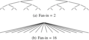
(a) Fan-in = 2
(b) Fan-in = 16
Fig. 2. Four balanced aggregation trees with 16 leaves.
III. MODELINTUITION ANDDEFINITIONS
In this section we explain the compute-aggregate model and what it means to have blocks versus streaming input.
A. Compute-Aggregate Problems
We consider how to to find a(c(z1), . . . ,c(zn)), which will
be formally detailed later in this section. Intuitively, each computation node contains some subset of the intial data. After computation (c), a system aggregates (a) the results along an
aggregation tree (or henceforth simply tree) communication
structure to create the final output. With the exception of passing the results of the computation to the aggregation tree the two phases are independent from each other. The two phases are visually represented in Figure 1.
We consider optimizating the aggregation phase. Optimizing computation requires knowledge about the data, data structures, and computation for each specific problem. We show optimiz-ing the tree often only requires knowoptimiz-ing very basic information about the aggregation function.
At each leaf, datazis in memory prior to computation, and computation applies functioncsuch thatx=c(z), wherexis data formatted for aggregation. There is no requirement on the type or complexity of the computation. It can be as simple as reading data from a source, such as a log file.
Aggregation can be triggered by the completion of the computation phase or run periodically on the current state of the data, as long as the data is formatted for aggregation. Aggregation applies some function a to all of the outputs of the computation nodes,a(c(z1), . . . ,c(zn)). This does not have
exactly once, resulting in an explicit tree structure. Figure 2 shows how 16 leaf nodes can be placed in two different trees with fan-ins of 2 and 16. These are the extreme scenarios, and it is possible to use any fan-in between the two values, although such fan-ins will not result in full trees unless the number of leaf nodes is a power of the fan-in.
Later in Section IV-B2 we discuss the idea of “implicit” ag-gregation. If portions of the data do not interact with each other, like subsequent chunks n-gram counting with no overlapping n-grams, but have an implicit order based on their locations in the input streams the tree may aggregate them separately without explicitly requiring them to be aggregated through the same channels as long as the ordering is maintained.
B. Single Block
The first case we consider is input processed in a single block, and each aggregation results in a single block of its own. This means all of the data is available and computed at a single step at the leaves, then the aggregation tree reads the entire results and outputs a single output without natural breaks which can be used to distribute the work.
In this case we are concerned with the optimal latency of processing the block. The number of inputs – including the direct outputs from the computation phase and aggregations of them – that can be aggregated at each node in the tree is variable, as long as each result from the computation phase is included exactly once. Reducing the fan-in means increasing the number of siblings in the tree, which in turn means that more aggregation is done in parallel at each level. However, subsequent levels have to repeat some of the work their children did. Therefore the optimal fan-in depends on the ratio of work that is repeated to the amount of parallelism gained.
C. Streaming
While the trees we will propose for single blocks of input are provably good, they only use one level of the aggregation tree at a time. Thus we consider a second case of input using multiple levels at a time. In order to do this we split the input into chunks according to rules laid out later in this section. By splitting the input we allow aggregation on some segment of the input data to be propagated up the tree while aggregating the next chunk at the lower levels. Thus we utilize more nodes in parallel. While this approach may recompute portions of the aggregation in a way that was avoided in the single block case, the additional parallelism can overcome that.
Rather than consider optimal latency per chunk we note that for any sufficiently large finitely sized input the optimal latency will be on a tree which has the highest bandwidth of processing the chunks. Of course, this extends to infinitely sized input as well, i.e. continuous input, and incrementally updated data where the results of the aggregation are updated, or even fed back into the original data for reaggregation.
We note that if a single block of input is sufficiently large it may be chunked and turned into a streaming problem if the data is amenable to such an operation, which means the input follows rules we define later in this section. In practice the
TABLE I NOTATION USED.
Token Meaning
n Number of computation/leaf nodes.
f Fan-in of the tree, making the height logfn.
a(x) The aggregation function for a set of inputs x.
at(x) Returns the time taken fora(x)(with communication).
t Time per unit of data for linearat(x)andat(/0) =0.
x0 Output from a computation node.
y Ratio of output sizes of consecutive levels.
y0 Ratio of the final aggregate output size to|x0|.
r(a,b) T RU Eiff itembfollows itemawith ordering functionr().
m A single chunk in a streamed input.
input must be sufficiently large to overcome the warmup and cooldown times of the tree, and for the increased parallelism used to increase the bandwidth of the streaming situation to overcome the reduction in latency with respect to one block.
D. In-Memory Data
Like the recent big data processing methods in our prior art search, we use in-memory computation (and aggregation). Because we are worried about high performance, disk accesses are a significant penalty on today’s hardware. In addition, mix-ing RAM and disk swappmix-ing leads to unpredictable latencies which can differ by orders of magnitude.
RAM constraints may be one thing that forces the use of the streaming model in practice. If the input size is too large to fit on a single machine, it will require chunking. Even if there are not enough chunks to overcome the warmup and cooldown phases, this may be preferable to requiring disk access.
E. Notation and Assumptions
We rely on several assumptions to calculate optimality. These do not affect the correctness of the output. Table I shows the notation used to rigorously define our assumptions and prove optimal fan-ins for the trees.
We assume time complexities of aggregation functions depend solely on input size. Some aggregation algorithms have time complexities expressed in terms of the fan-in and the size of individual inputs, e.g.O(f an-in×log(average input size)). Our experiments show this deviation is a small factor.
a pseudo-synchrony which requires a degree of homogeneity among nodes of a level. Heterogeneity may exist across levels. We do ignore some of the other complexities that can be associated with communication, especially with regard to node location on the network and shared resources or conflicts. We are considering mostly the case of using third party cloud offerings, which often hide such things from the user. As such we consider the network architecture a black box best approximated in the average case as mostly uniform.
Homogeneous hardware is a fair premise when datacenters mass order standard hardware, and cloud services provide tiers of service based on performance. The minor service variations can be unpredictable. Homogeneous input follows from our model for data distribution. If aggregation time depends on the data traits other than size (e.g., element order), those traits must be distributed. We find the leeway in synchrony and the impact of tree customization mask enough hetergeneity in practice.
Aggregation costs are modeled as monotonically increasing on input size, and are zero for no input. Modeling non-linear setup overheads complicates analysis, and the practical impact of these overheads are very small. When aggregation changes the size of the data we model ratio of output to input at each level to be the same. This is or can be made to be true for many applications. In many other cases the ratio stays within a range, e.g. below 1, and the optimal fan-in is unaffected.
We assume the same ideal fan-in is used at all levels of the tree as possible. Without a rigorous proof of this, we note that onceyis applied to the first level the optimal remaining fan-in is essentially being applied to 1f nodes with input different by a factor of y, which is essentially the same problem.
We model full and balanced trees. Fulfilling fullness for arbitrary numbers of leaves can be difficult, as it requires the fan-ins at each level to multiply to the number of leaves. It is simple to balance within a level, however, and fullness and balance follow when the number of leaves is a power of fan-in.
F. Function Requirements
We consider aggregation functions which takex1. . .xi and
output an aggregate x1..i, i.e., x1..i=a(x). Functions must be able to handle any number of inputs in order for the increased fan-in to be effective, as there is no advantage to having multiple inputs available it they cannot be used.
Functions are cumulative, commutative, and associative. This essentially means inputs may be aggregated in any order with any group of inputs, including those which are outputs of non-root nodes of the tree. Definitions 1, 2, and 3 capture the properties more precisely. Definitions require equivalency (≡), not necessarily identical output. For example, if a system is supposed to output the single word with the maximum number of occurrences (word count) and two words are tied for that distinction, either word may be returned.
Definition 1 (Cumulative Aggregation). a(a(x),a(x0))≡ a(x,x0)
Definition 2 (Commutative Aggregation). a(x0,x)≡a(x,x0)
Definition 3 (Associative Aggregation). a(a(x,x0),x00) ≡ a(x,a(x0,x00))≡a(x,x0,x00)
Because our streaming model outputs results before receiv-ing the entirety of the input, there are additional rules on the inputs which must be satisfied. This applies both to the original input and the output of nodes which is used as input higher in the tree. The inputs must all use a known ordering function, and side effects can only propagate from earlier chunks of data to later chunks rather than the opposite way around, as one would expect. Definitions 4, 5, and 6 define these in more rigorous language. We also provide counterexamples to each rule using a word count application.
Definition 4 (Known Ordering). ∃ some known transitive function r on pairs of keys s.t. for any pair k16=k2 of keys r(k1,k2)returns T RU E iff k1≤k2.
Counterexample: If the input is a hashmap with string:key
mappings, the ordering of a traversal of the list of entries is not a lexical ordering of the keys, but a numerical ordering of the hashes of the keys. The programmer must understand the datastructure and account for this.
Definition 5 (Consistent Ordering). ∀keys k1,k2 such that k1 precedes k2 in ordered list ci used as input for aggregation
function a(x0, . . . ,xd), if k1,k2⊂xj =⇒ rj(k1,k2) =T RU E.
Counterexample: One list could be derived from a
hashmap, ordered on the hashes of the keys. Another list may have been processed to follow lexical ordering of the keys or be sorted on the number of occurrences of each string.
Definition 6(Unidirectional Side Effects). In aggregation func-tion a(x0, . . . ,xd), list xican be decomposed into concatenated
lists x0i·x1i·x2i and xj into x0j·x1j·x2i for i6=j such that for any
element l0⊂x0and l1⊂x1, r(l0,l1).
If aggregation function a()is applied to chunks x0i and x0j to create output x0a,∃ items k01,k02⊂x0a such that r k01,k0
2
=
T RU E, then ax0i...2, . . . ,x0j...2 contains k10,k20⊂ x1a...2 such that r k01,k02=T RU E.
Counterexample: If the output is ordered on the number
of occurrences of each string, but stringsoccurs inx1
i and x2j,
the value used in the ordering ofs, and thus the ordering ofs relative to other elements, can change whenx2j is aggregated with the output from the original aggregation.
IV. OPTIMALITYPROOFS ANDMECHANISMS
A. Single Block Optima
Here we prove theoretical (near-)optimality of the fan-in f for minimizing latency givenn andat(x)for several cases of
y0when there is a single block of input at each tree leaf.
Lemma 1. The total aggregation time with linear at(x)
and y06=1 is g(f,n,y0) = t|logx0|f nf√(yy00−−11), and ∂
∂fg(f,n,y0) = t|x0|(y0−1)y
logn d
0 −
1+loglognyylogn f
ylog0 n f−12
Proof. For aggregation linear on input size, the time at a level is constantt×(the input size at the level). Initial input size is |x0|, and size changes by a factor ofyat each of the subsequent logfn levels. Thus total aggregation time is ∑zlog=1fnt f yz−1x0.
Pulling out the constants givest f|x0|∑ logfn z=1 yz
−1=tx0f ylogf n−1 y−1 . Recalling y= logf n√y
0gives t
|x0|f(y0−1) logf n√y
0−1.
Lemma 2. The total aggregation time with y0 = 1 is at(f|x0|)logfn.
Proof. Reusing the logic from Lemma 1 without introducingy0
gives us∑ logfn
z=1 at(f|x0|). This simplifies toat(f|x0|)∑ logfn z=1 1, and then to at(f|x0|)logfn.
Theorem 1. The optimal fan-in is2when y0<1and at(x)is linear or superlinear.
Proof. By Lemma 1, the total aggregation time
taken is g(f,n,y0) = t f
|x0|(y0−1) logf n√y
0−1, and ∂
∂fg(f,n,y0) is
t|x0|(y0−1)
ylog0 n f−1+ylog0 n flogny0
ylog0 n f−12
. 0 < lognf ≤ 1 for
2≤f ≤n, so ∂
∂fg(f,n,y0)>0 for 0<y0<1.
∴ The optimal f is 2.
We assumed at(x0) +. . .+at(xz) =at(x0+. . .+xz). As f
grows there are more inputs and input size is reduced less, and at(x0) +. . .+at(xz)<at(x0+. . .+xz) for superlinear at(x),
so superlinear at(x) is more sensitive to f than linearat(x). ∴ This result holds for superlinearat(x).
Theorem 2. The optimal fan-in is e when y0=1 and at(x)is linear.
Proof. Withat(f|x0|)logfnfrom Lemma 2 and linearat(x),
g(f,n,y0) = f|x0|tlogfn. ∂∂fg(f,n,y0) =
|x0|t(logf−1)logn
log2f ,
which is 0 iff f =e. ∂2
∂f2g(f,n,y0) =−
|x0|t(logf−2)logn flog3f . At
f=e, ∂2
∂f2g(f,n,y0)>0, so this is a minimum.
∴ The optimal f ise.
Theorem 3. The optimal fan-in is[2,e)when y0=1and at(x) is superlinear.
Proof. By Lemma 2 the total aggregation time is
glinear(f,n,y0) =at(f|x0|)logfn. As shown in Theorem 2,
limat(x)→linear is e. We can assume ∂
2
∂f2gsuperlinear(f,n,y0)> ∂2
∂f2glinear(f,n,y0). Thus ∂ 2
∂f2glinear(f,n,y0) > 0 for
f ≥e =⇒ ∂2
∂f2gsuperlinear(f,n,y0)>0. Thus any minimum occurs at f <e. ∴ The optimal value of f is in the range
[2,e)
Theorem 4. The optimal fan-in is (1−logny0)
−logy0n when
1<y0<n and at(x)is linear.
Proof. From Lemma 1, the amount of time taken to
aggregate is g(f,n,y0) = t f
|x0|(y0−1) logf n√y
0−1, and ∂2
∂f2g(f,n,y0) =
t|x0|(y0−1)
ylog0 n f−12
ylognf
0 −
1+ylognf
0 logny0
. For
y0>1, t
|x0|(y0−1)
ylog0 n f−12
>0, so the expression is 0 iff ylognf
0 =
1+ylognf
0 logny0
, which happens at f = (1−logny0)−logy0n.
∂2
∂f2g(f,n,y0) =
t|x0|(y0−1)y logn f 0 logy0
logn+logy0−(logn−logy0)y logn f 0
flog2nylogn f
0 −1
3 . Because
t|x0|(y0−1)ylog0 n flogy0 flog2nylogn f
0 −1
3 >0, ∂ 2
∂f2g(f,n,y0)>0 iff logn+logy0−
(logn−logy0)ylog0 nf >0. Substituting the extrema value for
f gives y
−logy0(1−logn y0)
0 −1
y
−logy0(1−logn y0)
0 +1
−logny0<0. To prove this we fix n
and findy0to maximizeh(f,y0) =
y
−logy0(1−logn y0)
0 −1
y
−logy0(1−logn y0)
0 +1
−logny0.
∂
∂y0h(f,y0) =
2 log2n+log2y0−4 lognlogy0 y0logn(logy0−2 logn)2
. ∂
∂y0h(f,y0) > 0 for 1 < y0 < n. Thus max(h(n,y0)) occurs at limy0→n, and limy0→nh(n,y0)<0. The extrema ofg(f,n,y0)is a minimum.
(1−logny0)−logy0n>n =⇒ d>n, which is impossible. Since the only local extrema is a minimum, ∂
∂fg(f,n,y0)<0
for f =h2,(1−logny0)−logy0n i
, so the optimal fan-in is the largest possible value, i.e.n, in this case.
∴The optimal f ismin(n,(1−logny0)−logy0n).
Theorem 5. The optimal fan-in is n when y0≥n.
Proof. The time taken by the root node isatylogfn|x
0|
.y0≥ n =⇒ y≥f and logfn≥1, so this is minimal at logfn=1. In addition, for f <nthe rest of the tree takes non-zero time. ∴The optimal f is n.
Table II summarizes the results from our proofs. There are still unproven cells where the degree of sub- or superlinearity of the aggregation is required to find the optimal value. There is always an aspect of linearity toat(x)due to communication time, so it makes sense to use the results from the linear cases on the sublinear cases, which would fill most of the table.
B. Streaming Optima
The case for streaming input is different than a single block. In this case we are worried about the bandwidth instead of the latency. As such, we explore the tree which can process subsequent input chunks the fastest. Intuitively this means finishing the initial processing of the current chunk the fastest so the tree can start processing the next chunk.
TABLE II
THE OPTIMAL VALUE FORfTO MINIMIZE THE LATENCY OF A SINGLE INPUT BLOCK AND THE APPLICABLE PROOF WHEN AVAILABLE.
y0 Model Runtime Optimal Fan-in Sublinear at() Linear at() Superlinear at()
y0<1
t|x0|f(y0−1)
logf n√y0−1 2 unproven Theorem 1 Theorem 1
y0=1 t f|x0|logfn e unproven Theorem 2 Theorem 3 (near optimal)
1<y0<n t|x0|f
(y0−1)
logf n√y0−1 min
n,(1−logny0)−logy0n
unproven Theorem 4 unproven
y0≥n t|xlog0|f nf√(yy00−−11) n Theorem 5 Theorem 5 Theorem 5
Theorem 6. The maximal bandwidth for streaming input when the entire tree keeps pace with the first level of aggregation happens when the f =2at the first level.
Proof. Bandwidth is throughput per time unit. Assuming the
rest of the aggregation tree keeps pace with the lowest level, we only have to consider the bandwidth of the lowest level. The throughput is equal to the amount of input, which is|m|at each of n nodes. The latency of the first level isat(x)where |x| is f×m. This makes the bandwidth ant|(mx|). By definition
at(x)monotonically increases with input size, so for a given mthe the denominator is minimized by minimizing f. ∴ The optimal f at the lowest level of aggregation is 2.
It is interesting to know that while this result is independent of the degree of function at(x), there is an additional implied
optimization that is possible in the case the function is not linear on|m|. Because the numerator is linear on|m|, sublinear occurrences in the denominator mean that |m| should be maximized. Similarly |m| should be minimized when the aggregation cost function is superlinear on |m|. In the case the function is linear, |m| does not affect optimality.
As long as y0≤1 an entire tree with f=2 will keep pace with the first level: simply create the rest of the tree with f=2 as well. Since the output of each level is not growing, each level has no more aggregation work to do than the level below it. Thus no level is a bottleneck compared to its level below.
Ify0>1 this does not work. Each level takes longer than the level below it, so input will buffer in ever increasing amounts between levels. Eventually it will be necessary for lower levels to wait to send the next because the levels to which they are sending will not be able to store it.
We propose two mechanisms to better use the computational power of the tree.
1) Modifying Chunk Size: The first mechanism prevents
buffering which could lead to buffer overloads when y0>1 and ameliorates some warmup and cooldown inefficiencies: rather than fixing |m|, we change the size of each chunk. If each subsequent chunk is a factor of ylarger each level takes as long to aggregate a chunk as the next level up takes to aggregate the previous chunk.
In practice it is impractical to increase the size of chunks indefinitely. Therefore we suggest specifying a minimum and maximum chunk size. Ify0>1 start with the minimum chunk size. Chunk sizes are increased until the maximum size is encountered, which will take logyMAXMIN((||mm))|) iterations.
The tree requires the occasional cooldown period clear to let the largest chunk propagate through the tree before the aggregation power is available to the next chunk. There is also a warmup period when the first chunk, or the smallest chunk when the chunk size is reset, propagates through the tree. When the chunk size is reset these two periods can overlap, but the warmup phase cannot overtake the cooldown phase because the hardware is not available. It is not necessary to know the exact value ofy a prioriin this case. The first level of aggregation can use the size that it is outputting for a chunk divided by the original size of the input for that chunk.
Since the tree must still wait when resetting the size of the chunks this is not perfectly ideal. However, the waiting is predictable rather than occurring whenever the buffers happen to fill up. In addition, since it handles several chunks before bogging down it may be sufficient for bursty streams.
2) Modifying Fan-in: When y0<1, aggregation happens
faster higher in the tree due to decreasing input size. Levels of the tree above the first are underutilized after finishing aggregation but before receiving the next chunk. The previous mechanism shifts this wait time to when chunk size resets, but does not alleviate it completely. Since we are using the proven optimal bandwidth in this case, there is no opportunity to improve bandwidth. Rather, this suggests that we can get comparable performance with less hardware.
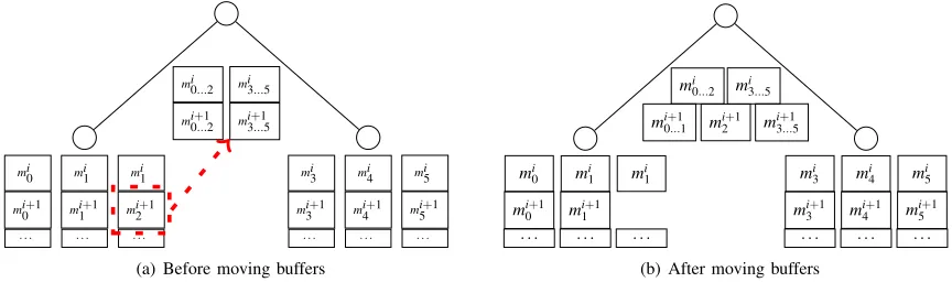
To address this we consider how to implement higher fan-ins, even fractional fan-ins. This is not possible with single chunks because there is no way to break up a chunk in the middle. However, with streaming input we already have natural breaking points. Figure 3 shows how we can use these to move aggregation to different points in the tree. In the figure the lower level aggregates 3 inputs, and the higher level aggregates the results from those two nodes. Assume the higher level is completing its work faster than the lower level. As a response it takes a chunk away from one of its children. As a result, in the i+1 step the top node has more aggregation to slow it down, and the child only has two inputs for that chunk, speeding it up. This means that the higher level has a higher effective average fan-in than the original 2, and the child which transferred a chunk has a lower one that the original 3.
mi0...2 mi
3...5
mi+1
0...2 mi3+...15
mi
0
mi+1
0
. . . mi
1
mi+1
1
. . . mi
1
mi+1
2
. . .
mi
3
mi+1
3
. . . mi
4
mi+1
4
. . . mi
5
mi+1
5
. . .
(a) Before moving buffers
mi
0...2 m
i
3...5
mi+1 0...1 m
i+1
2 m
i+1 3...5
mi
0
mi+1 0
. . .
mi
1
mi+1 1
. . .
mi
1
. . .
mi
3
mi+1 3
. . .
mi
4
mi+1 4
. . .
mi
5
mi+1 5
. . .
(b) After moving buffers
Fig. 3. Fractional fan-in through buffer transport.
on demand. When a node detects it is running low on buffered chunks, it asks a child to transfer one. It asks the child which seems to be the furthest behind, since this will speed up the subtree of that child. This dynamically balances the tree.
Another limitation is that the requested chunk cannot be aggregated as it is received. Rather, the chunk must be buffered until the other chunks from the ith step are received. This means that the speed up or slow down at a node from sending or receiving a chunk will not be seen immediately.
Initial input chunks can be filtered immediately into the tree, and the full tree may be fully utilized as soon as the initial warmup phase is complete. This does open the possibility of fan-ins below 2 at the lowest level, which would theoretically decrease per-chunk latency and increase bandwidth. Perhaps a user could actually specify a number of available nodes and increase bandwidth by creating an effective fan-in below 2 at the lowest level, but we do not explore this.
A more practical use of this is choosing a size of tree which has different fan-ins at each level and balancing the effective fan-in at each level with this mechanism. We can thus create trees which have effective fan-ins of exactly the calculated optimum, even if that optimum is fractional. This means having a complete and fully utilized tree, giving us the performance which can match the performance of a fan-in of 2 at the lowest level with the lowest number of nodes, thus decreasing the cost to maintain a system implementing this.
This approach allows the rest of the tree to keep pace with the lowest level even for y0>1 if one additional property is met: aggregation must include no side effects, as precisely captured by Definition 7. This is reasonable for applications such as n-gram counting and merging time sorted lists where chunking is done on preselected time values.
Definition 7 (No Side Effects). In aggregation function a x0, . . . ,xf
, list xican be decomposed into concatenated lists
x0i ·x1i·c2i and xj into x0j·x1j·x2i for i6=j where the chunking
happens on some delimiter s.
If aggregation function a()is applied to chunks x0i and x0j to create output x0a, then x1i and x1j to derive output x1a, and a()is applied separately to only x1i and x1j to derive output x0a1, x1a≡x0a1.
With this we can build side-by-side trees to handle different
chunks. For example, one tree may take even numbered chunks, and another take the odd chunks, reducing the work of a tree by a factor of two. The order of the chunks imparts an implicit aggregation that requires no work to maintain explicitly.
V. EVALUATION
To evaluate the model we run several microbenchmarks on a set of m1.medium nodes in an Amazon EC2 datacenter. We run a tightly controlled compute-aggregate solution compare the results against the modeled expectations. The compute phase consists of randomly generating a set size of integers. The aggregation at each node receives a set of lists from its children and performs some rather intensive computation which takes time which is almost perfectly linear on the total input size to produce an output list of integers which is a factor of the givenydifferent from the average size of its inputs.
A. Single Block
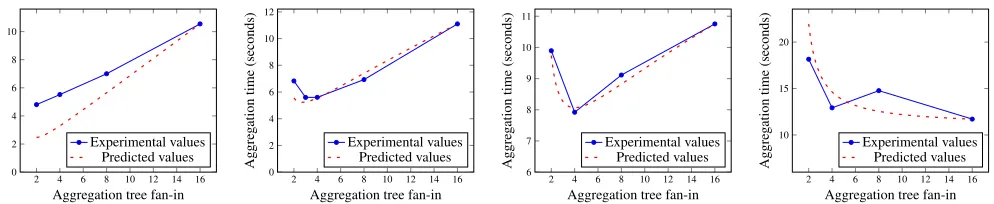
Figure 4 shows the latency of running our microbenchmarks for a single block of input on 16 nodes with an initial input size of 100000 items. We vary the fan-in from the minimum value of 2 to the maximum value ofn. We use a bottom-to-top greedy algorithm to assign node placement. That is, the bottom most level is filled up as much as possible from left to right. When there are no more nodes to act as children at that level, we move to the next level up.
Each graph has a line of “Predicted values” which is a line generated by the appropriate mode with the constants set so it goes through the point when f =16. In general, the trends predicted by the model are seen in the data. The minima occur close to the predicted places. We note that the actual optima do vary from 2 ton depending on y0, so there is no constant optima. The difference in choosing the optimal fan-in and the worst case scenario is always at least 40%, and the predicted optima always the experimental optimum in these conditions. We use 3 to approximate e.
2 4 6 8 10 12 14 16 0
2 4 6 8 10
Aggregation tree fan-in
Aggre
g
ation
time
(seconds)
Experimental values Predicted values
(a) Experiment vs. predicted,y0=1n
2 4 6 8 10 12 14 16
0 2 4 6 8 10 12
Aggregation tree fan-in
Aggre
g
ation
time
(seconds)
Experimental values Predicted values
(b) Experiment vs. predicted,y0=1
2 4 6 8 10 12 14 16
6 7 8 9 10 11
Aggregation tree fan-in
Aggre
g
ation
time
(seconds)
Experimental values Predicted values
(c) Experiment vs. predicted,y0=
√ n
2 4 6 8 10 12 14 16
10 15 20
Aggregation tree fan-in
Aggre
g
ation
time
(seconds)
Experimental values Predicted values
(d) Experiment vs. predicted,y0=n
Fig. 4. Microbenchmark Results
a fan-in of 8 the lower level has the appropriate fan-in, but the top level only has a fan-in of 2. We note that this is still balanced. For other fan-ins this approach creates high levels of imbalance. Algorithms which strive for balance by starting top down appear to be possible, but they are more involved to implement than our greedy approach.
0 10 20 30 40 50 60
10 20 30 40 50
Aggregation tree fan-in
Aggre
g
ation
time
(seconds)
Experimental values Predicted values
Fig. 5. Scalability test withy0=1 and n=96.
0 5 10 15 20 25 30 35
0 5 10 15 20
Fan-in
Aggre
g
ation
time
(seconds)
Fig. 6. Time for lowest level of
streaming with various fan-ins.
16 nodes is not a lot in cloud computing systems. Figure 5 extends the results for y0=1 to 96 nodes, which is more realistic. In these results we see an even bigger penalty for choosing a non-optimal fan-in. The difference beween the optimal fan-in and a fan-in of 64 is 500%. So choosing an optimal fan-in is more important for larger. We omit the data point for d=96 because at the input was not able to fit in memory at the root, and latency increased by almost an order of magnitude due to the time required for disk access. This just reinforces the idea of using a streaming model when possible with big data to avoid such problems.
B. Streaming
Figure 6 shows the latency of the lowest level of aggregation only for one chunk in streaming input. We remind the reader that as the fan-in increases there is no change the size of the output per set of chunks read in, so this merely increases the time unit. Thus the increase in latency corresponds directly to a decrease in bandwidth, and it is clear the optimal bandwidth occurs with minimal fan-in at the first level of aggregation.
For the streaming experiments with y0≤1 and fan-in of 2 at the lowest level of aggregation, an entire tree with fanout 2 sufficient to keep up. Figure 7 shows the number of nodes needed in total for such a tree with 32 at the lowest level as
0 0.2 0.4 0.6 0.8 1 30
35 40 45 50
y0
Nodes
Used
Naïve Approach Variable Fan-in
Fig. 7. Nodes needed for varying
fan-in vs. maintainingf=2.
0 5 10 15 20 25 30 35
0 20000 40000 60000 80000
y0
Throughput
(items/second)
Throughput without waiting Single sized|m|
MAX(|m|) = 1000×MIN(|m|)
Fig. 8. Throughput penalty of resetting the size ofm.
the naïve approach. The second line in the graphs shows the number of nodes needed if we instead use the approach in Section IV-B1 to create a variable fan-in tree.
Fractional fan-in above the first level is calculated based ony0 with minimal overhead to implement the chunk transfer function. We then determine the minimal number of nodes to implement that fan-in. Since we must have at least enough capacity to handle the flows, rounding is done up.
Neary0=1, there are no potential node savings. Removing a single node reduces the capacity of the tree to the point that the tree cannot keep up with its first level. As the output size of the first level decreases with respect to its input size the rest of the tree does not need as much computational ability to keep up to the extreme the point that it can use a single node. This reduces the number of nodes required by nearly a factor of two, although all the bottom level nodes are still required. This is beneficial for cost and maintenance savings.
Withy0>1, variable fan-in does not help unless Definition 7 is satisfied and the system can create parallel trees with implied ordering to handle different chunks of input. If that is not the case, we have to use decreasing chunk sizes with the occasional pause to allow the tree to cool down and warm up again as chunk size hits its limit and is reset.
by the level. Because the output size grows at each level, every level is waiting for the level above it. The bandwidth essentially becomes constrained by the root node.
The middle line comes from varying |m|. Maximum and minimum chunk sizes are chosen with a ratio of 1000:1. As the bottom level outputs an aggregated chunk, it reads a new chunk the same size as its output, which is a factor ofytimes larger than the previous chunk. When the maximum chunk size is hit, the tree simultaneously cools down and warms up the new smallest chunk using the same pausing strategy as used in the case with fixed chunk size. Each level waits until the level above it is ready to continue before continuing itself. Especially wheny0is not very large, this approach is better than using a single size chunk. However, there is still a penalty suffered from not having a tree which is able to keep up with the lowest level. This may be enough to handle bursty traffic where the cooldown and warmup may initiated early done during lapses in input. Otherwise this suggests a user should make efforts to abide by Definition 7 and build parallel aggregation structures when possible.
VI. CONCLUSIONS ANDFUTUREWORK
An infrastructure for efficient compute-aggregate applica-tions is a relevant advancement in big data computing. This can be done via intimate knowledge of the aggregation function in question, but that limits the applicability to a relatively small number of tasks. One of our goals is to identify universal characteristics of compute-aggregate tasks that allow to unify design principals of “ideal" aggregation trees.
We rigorously prove optimality of aggregation trees for two different cases of compute-aggregate systems. We lay out our systems of interest, the assumptions we make, and the conditions we impose. For processing a single block of input we explain that the appropriate measure is latency and that the ratio of output size to input size affects the optimal fan-in.
For streaming input, we fix the fan-in to 2 and focus on bandwidth because of the increased parallelism of the tree. To better exploit the parallelism we introduce two potential mechanisms to allow the tree to keep pace with the first level when possible – with reduced maintenance cost when appli-cable. These efforts are particularly useful when aggregation reduces the size of input, as in many real world applications. Our evaluation section uses microbenchmarks on simulated aggregation functions which are linear on input size to validate the model and explores the limits of the alterations to the streaming tree to maximize throughput.
Moving forward we are developing algorithms to produce relatively balanced trees when the number of nodes does not lend itself well to this using our current bottom to top greedy algorithm. We are also looking to see if using the degree of super- or sub-linearity of the aggregation function to further refine optimal values in those cases is worth pursuing or if the current rules are good enough given their ease to calculate.
REFERENCES
[1] CHANG, J.-H.,ANDTASSIULAS, L. Energy Conserving Routing in
Wireless Ad-hoc Networks. InAnnual Joint Conference of the IEEE
Computer and Communications Societies (INFOCOM)(2000), vol. 1, pp. 22–31.
[2] CHEN, Y., GANAPATHI, A., GRIFFITH, R.,ANDKATZ, R. The Case for
Evaluating MapReduce Performance using Workload Suites. InIEEE
International Symposium on Modeling, Analysis Simulation of Computer and Telecommunication Systems (MASCOTS)(2011), pp. 390–399.
[3] CHENG, Y.,ANDROBERTAZZI, T. Distributed Computation for a Tree
Network with Communication Delays.IEEE Transactions on Aerospace
and Electronic Systems, 26(3) (1990), pp. 511–516.
[4] COSTA, P., DONNELLY, A., ROWSTRON, A.,ANDO’SHEA, G.
Cam-doop: Exploiting In-network Aggregation for Big Data Applications. In
USENIX Conference on Networked Systems Design and Implementation (NSDI)(2012).
[5] DEAN, J.,ANDGHEMAWAT, S. MapReduce: Simplified Data Processing
on Large Clusters. Commun. ACM 51, 1 (Jan. 2008), 107–113.
[6] HUEBSCH, R., HELLERSTEIN, J. M., LANHAM, N., LOO, B. T.,
SHENKER, S.,ANDSTOICA, I. Querying the Internet with Pier. In
International Conference on Very Large Data Bases (VLDB) (2003), pp. 321–332.
[7] ABU-LIBDEH, H., COSTA, P., ROWSTRON, A., O’SHEA, G., AND
DONNELLY, A., Symbiotic Routing in Future Data Centers. InACM SIGCOMM Conference, (2010), pp. 51–62.
[8] JAIN, N., KIT, D., MAHAJAN, P., YALAGANDULA, P., DAHLIN, M.,
ANDZHANG, Y. Star: Self-tuning Aggregation for Scalable Monitoring.
InInternational Conference on Very Large Data Bases (VLDB)(2007), , pp. 962–973.
[9] KIM, H.-J., JEE, G.-I.,ANDLEE, J.-G. Optimal Load Distribution
for Tree Network Processors. IEEE Transactions on Aerospace and
Electronic Systems, 32(2), (1996), pp. 607–612.
[10] MADDEN, S. R., FRANKLIN, M. J., HELLERSTEIN, J. M.,ANDHONG,
W. TinyDB: An Acquisitional Query Processing System for Sensor
Networks. ACM Trans. Database Syst., 30(1), (Mar. 2005), pp. 122–
173.
[11] MOROZOV, D., AND WEBER, G. Distributed Merge Trees. In
ACM SIGPLAN Symposium on Principles and Practice of Parallel Programming (PPoPP)(2013), pp. 93–102.
[12] MURRAY, D. G., MCSHERRY, F., ISAACS, R., ISARD, M., BARHAM, P.,
ANDABADI, M. Naiad: A Timely Dataflow System. InACM Symposium
on Operating Systems Principles (SOSP)(2013), pp. 439–455.
[13] TAN, H. O.,ANDKÖRPEO ˇGLU, I. Power Efficient Data Gathering and
Aggregation in Wireless Sensor Networks.SIGMOD Rec., 32(4), (Dec.
2003), pp. 66–71.
[14] VANRENESSE, R., BIRMAN, K. P.,ANDVOGELS, W. Astrolabe: A
Robust and Scalable Technology for Distributed System Monitoring,
Management, and Data Mining.ACM Trans. Comput. Syst., 21(2), (May
2003), pp. 164–206.
[15] VENKATARAMAN, S., ROY, I., AUYOUNG, A.,ANDSCHREIBER, R.
Using R for Iterative and Incremental Processing. InUSENIX Workshop
on Hot Topics in Cloud Computing (HotClouds)(Jun 2012).
[16] WU, H., FENG, Z., GUO, C., AND ZHANG, Y. ICTCP: Incast
Congestion Control for TCP in Data-center Networks.IEEE/ACM Trans.
Netw., 21(2), (2013), pp. 345–358.
[17] YALAGANDULA, P.,ANDDAHLIN, M. SDIMS: A Scalable Distributed
Information Management System. In ACM SIGCOMM Conference
(2004).
[18] YANG, H.-C., DASDAN, A., HSIAO, R.-L.,ANDPARKER, D. S.
Map-Reduce-Merge: Simplified Relational Data Processing on Large Clusters. InACM SIGMOD International Conference on Management of Data (SIGMOD)(2007), pp. 1029–1040.
[19] YU, Y., GUNDA, P. K.,ANDISARD, M. Distributed Aggregation for
Data-Parallel Computing: Interfaces and Implementations. In ACM
SIGOPS Symposium on Operating Systems Principles (SOSP)(2009), pp. 247–260.
[20] ZAHARIA, M., CHOWDHURY, M., DAS, T., DAVE, A., MA, J., MC
-CAULEY, M., FRANKLIN, M. J., SHENKER, S.,ANDSTOICA, I. Re-silient Distributed Datasets: A Fault-tolerant Abstraction for In-memory
Cluster Computing. In USENIX Conference on Networked Systems
Design and Implementation (NSDI)(2012), pp. 2–2.
[21] ZHANG, Y.,ANDANSARI, N. On Architecture Design, Congestion
Notification, TCP Incast and Power Consumption in Data Centers.IEEE