Air Pollution Dispersion Modelling Using Spatial Analyses

Article

AIR POLLUTION DISPERSION MODELLING

USING SPATIAL ANALYSES

Jan BITTA1,2 ID_{, Irena PAVLÍKOVÁ}1,2,3_{,Vladislav SVOZILÍK}2,3,4_{and Petr JAN ˇCÍK}1,2,3

1 _{Department of Environmental Protection in Industry, Faculty of Metallurgy and Material Engineering, VSB}

-Technical University of Ostrava„ 17.listopadu 15/2172, 708 33, Czech Republic, Kat616@vsb.cz

2 _{Institute of Environmental Technology (IET), VSB - Technical University of Ostrava, 17.listopadu 15/2172,}

708 33, Czech Republic

3 _{Joint Institute for Nuclear Research (JINR), Joliot-Curie 6, 141980 Dubna, Moscow region, Russia,}

svozilik@jinr.ru

4 _{Institute of Geoinformatics, Faculty of Mining and Geology, VSB - Technical University of Ostrava,}

17.listopadu 15/2172, 708 33, Czech Republic

* Correspondence: Kat616@vsb.cz; Tel.: +420 597 324 346 † Current address: Affiliation 3

‡ These authors contributed equally to this work.

Abstract:The air pollution dispersion modelling via spatial analyses (Land Use Regression – LUR) is an alternative approach to the air quality assessment to the standard air pollution dispersion modelling techniques. Its advantages are mainly much simpler mathematical apparatus, quicker and simpler calculations and a possibility to incorporate other factors affecting pollutant’s concentration. The goal of the study was to model the PM10 particles dispersion modelling via spatial analyses v in Czech-Polish border area of Upper Silesian industrial agglomeration and compare results with results of the standard Gaussian dispersion model SYMOS’97. Results show that standard Gaussian model with the same data as the LUR model gives better results (determination coefficient 71% for Gaussian model to 48% for LUR model). When factors of the land cover and were included into the LUR model, the LUR model results were significantly improved (65% determination coefficient) to the level comparable with Gaussian model. The hybrid approach combining the Gaussian model with the LUR gives superior quality of results (65% determination coefficient).

Keywords:Pollution dispersion; PM10; air quality; Land Use Regression; Symos’97

1. Introduction

1.1. Particulate pollution

The PM (Particulate matter) is called a mixture of solid or liquid both organic and anorganic substances in the air. It mainly consists of sulfates, nitrates, ammoniac, salts soot, mineral particles, metals, bacteria, pollens and water. Particles of diameter smaller than 10µm (PM10) have severe health

effects because they may get into lungs or even join the blood stream [19], [20],[16].

Figure 1.Illustration of PM10 and PM2.5 size [19]

Natural PM10sources are forest fires, dust storms, volcanic processes, erosion or sea water [3],

[11]. Large part of PM10 has anthropogenic origin [22]. It consists of combustion processes (thermal power plants, heating, internal combustion engines), industrial processes like coking, blast furnaces, steelworks, sinter plants, cement production or mineral extraction, dust resuspension from roads and agriculture (soil erosion) [16], [17], [9], [8]. Recent research indicates non-existence of a minimal

threshold concentration value for human health effects [3]. Factors influencing health effects are

particles’ size and geometry, their chemical composition, physical properties, concentration and time of exposure. Particles greater than 10µm are caught by ciliated epithelium of upper respiratory tract and

have low health impact. Particles smaller than 10µm cumulate in bronchi and lungs and cause health

issues. Particles smaller than 1µm possess the biggest health threat because they may get into alveoli

and frequently contain adsorbed carcinogenic substances. The PM10inhalation damages mainly heart

and lungs and is a cause of premature death of people with heart or lung disease, cancer, fibrosis, allergic reactions, asthma, lung insufficiency, heart attacks, respiratory tract irritation and cough [19], [20],[16], [3], [11]. There are two legal pollution limits for PM10. The 24-hour average limit is 50µg/m3 which can be exceeded no more than 35 times per year. The annual average concentration limit is set as 40µg/m3[13],[14].

1.2. Land Use Regression modelling

The Land Use Regression (LUR) modelling is an empirical modelling approach which is based on multivariate linear regression. It combines pollution monitoring data with spatial variables describing vicinity of monitoring sites which are typically obtained via spatial analyses in Geographic Information Systems (GIS). The result of the analyses is the linear model

where[Factor-∗]are selected spatial factors and[Coe f_∗]are regression coefficients obtained from the linear regression analysis at the pollution monitoring sites. The empirical model can be than used to estimate spatial distribution of the PM10 pollution in the area of interest. The LUR model was first used for the air pollution monitoring in the SAVIAH (Small Area Variations in Air quality and Health)

project. This approach was used to study NOxconcentrations in three European cities – Amsterdam,

Huddersfield and Prague. The successful application of the LUR in the SAVIAH project model spurred its usage in further studies in European countries and in the rest of the world [10], [15],[12].

1.3. Gaussian dispersion modelling

Gaussian dispersion models assume an emission transport from continuous pollution sources in homogenous wind field without spatial limits. The transport itself is in the model provided by the convection by wind and via turbulence diffusion which is described statistically by Gaussian distribution. Spatial limitations, mainly the terrain, are included into model by correction coefficients. Gaussian dispersion models are commonly used for long term (f.e. annual) average concentrations modelling. The dispersion is calculated for a set of standard meteorological conditions and summed, weighted by probability of occurrence of such conditions. The most commonly used Gaussian

dispersion models are CALINE3 (Benson, 1979) and ADMS-Urban [1]. The SYMOS’97 model [18] is a

reference pollution dispersion model in the Czech Republic. It is a Gaussian model which calculates pollution dispersion of both gaseous and particulate pollutants from point, linear and area pollution sources. The model takes into account both dry and wet deposition as well as chemical reactions during transport.

2. Data sources

The study area was selected to match the area of the Air Silesia project [2]. All air pollution source and monitoring data used in the study were purchased from published results of the Air Silesia project and are relevant to the year 2010. The Air Silesia project was focused on collecting the air pollution data and assessment of the air quality in the border region of the Upper Silesian industrial region.

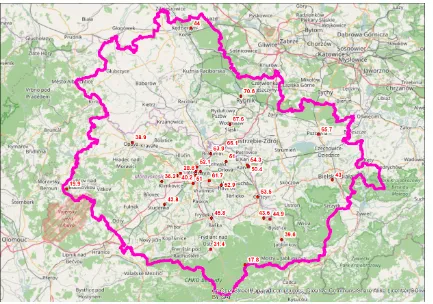
The following Fig. 2 shows the study area and the annual mean PM10 concentrations [µg/m3] at the

Figure 2.The study area and pollution monitoring stations with annual average of PM10

Figure 3.Annual mean PM10 concentrations in 2010 [6].

2.1. Air pollution data

The air pollution data – yearly averages of PM10concentrations, were obtained from the yearbooks

[5] of the Czech Hydrometeorological Institute and the Voivodship Inspectorate of the Environmental

2.2. Pollution source data

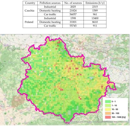
The pollution source data were obtained from the pollution source database provided by the Air Silesia project. The data have been divided by the land of origin (Czech-Polish) and by the kind of the pollution source (industrial, domestic heating, car traffic). Brief statistics of emissions are presented in following Tab.1 and emission squares (Fig. 4)

Table 1.The PM10 pollution sources in the study area, (Air Silesia, 2013)

Country Pollution sources No. of sources Emissions [t/y]

Czechia

Industrial 2025 2315

Domestic heating 21824 1589

Car traffic 56057 961

Poland

Industrial 1598 13400

Domestic heating 33301 8610

Car traffic 55745 911

Figure 4.The PM10distribution in the study area, Basemap:OpenStreetMap

2.3. Land Use data

The land use data were obtained from the CORINE Land Cover dataset [7] as vector datasets.

There were four kinds of land cover selected for the analysis – built-up areas, forested areas, areas with grass cover and open soil-agricultural areas.

3. METHODOLOGIES AND RESULTS

monitoring stations. The factor was than calculated as a sum, percentage or length-weighted average of the vector data cut by the buffer. Factors were calculated uniformly (U) or they were calculated as a weighted average based on wind direction probability (W). The area of modelling was split into 14 areas according to the terrain configuration. Meteorological condition in each area were represented by its own dataset (Fig. 5). In that case, buffer zones were split into 8 slices representing 8 wind directions. Factors were calculated for each slice area and final weighted factors were calculated as a weighted average of those factors where weights were probability of wind blowing from corresponding direction.

Table 2.Factors of pollution sources, factors of land cover

Factor Identifier sources Distances Weighing Unit Emissions from industrial sources IS 100,200,500,1000,2000 U,W t/y

Length of roads LR 100,200,500,1000,2000 U,W m

Average traffic intensity

weighted by length of road sections TI 100,200,500,1000,2000 U,W car/day Emissions from domestic heating DH 100,200,500,1000,2000 U,W t/y

Distance to the nearest road NR

Grass covered land GCL 100,200,500,1000,2000 U,W % of area Forested land FL 100,200,500,1000,2000 U,W % of area Built-up land BL 100,200,500,1000,2000 U,W % of area

Open soil OSL 100,200,500,1000,2000 U,W % of area

For the purpose of the study, all factors were encoded. For example, the[FL_500_W]code means the

factor of forested land cover counted for the buffer distance 500m and weighted by the wind direction probability distribution.

Regression analyses were performed in the Statgraphics software. The regression models were constructed for combinations of industrial sources([IS_∗_∗]), traffic intensity([T I_∗_∗]), domestic heating([DH_∗

hbox_∗]) and nearest road ([NR]). Regressions consisted of two steps, statistical

significance/insignificance of each factor was evaluated and regression coefficients were calculated with statistically significant factors. The best statistical analysis result was a regression model:

[PM10_concentration] =30.8507+0.00789643∗[IS_2000_W] +0.000583609∗[T I_2000_W]

+0.214567∗[DH_2000_W] +0.01368∗[NR] (2)

The R2of the model is 48% and mean quadratic error of the model is 10.59µg/m3. When factors of the land cover were taken into account, the resulting best linear model was constructed as

[PM10_concentration] =46.3802+0.00113242∗[IS_2000_W] +0.203484∗[DH_2000_W]

−0.299948∗[FL_1000_W] (3)

The R2of the model is 65% and mean quadratic error of the model was 8.34µg/m3.

● ● ● ● ● ● ● ● ● ● ● ● ● ● ● ● ● ● ● ● ● ● ● ● ● ● ● ●● ●

0 20 40 60 80

0 20 40 60 80 Observed Predicted

● Pollution sources model Pollution sources + Landcover model Model Symos'97 result

Figure 6.Observed to predicted comparison of results

The results of the SYMOS’97 model were statistically evaluated with the measurements at

monitoring sites. The R2 of the model is 71% and mean quadratic error of the model was 7.44

µg/m3. Both approaches, the LUR and the dispersion model, can be combined into a hybrid, two-step

There were two possible input tested. The land cover data were combined with both partial results of the model and the sum of all partial results.

Table 3.Factors based on dispersion model.

Pollution from industrial sources M_IS µg/m3 Pollution from domestic heating M_DH µg/m3 Pollution from road traffic M_RT µg/m3 Sum of all sourcesc M_SUM µg/m3

When the dispersion model results and factors of the land cover were taken into account, the resulting best linear model was constructed as

[PM10_concentration] =28.7086+0.155629∗[OSL_1000_W]−0.12583∗[FL_1000_W]

+3.50718∗[M_IS] +3.25479∗[M_DH] +6.75771∗[M_RT] (4)

The R2of the model was 86% and mean quadratic error of the model was 5.56µg/m3.

0 20 40 60 80

0 20 40 60 80 Observed Predicted ● ● ● ● ● ● ● ● ● ● ● ● ●● ● ● ● ● ● ● ● ● ● ● ● ● ● ●

Pollution sources + Landcover model Hybrid dispersion−LUR model

Figure 7.Observed to predicted comparison of results

The dispersion model provides more accurate information about pollution dispersion from pollution sources and the LUR model allows incorporation of additional variables

4. DISCUSSION

The LUR model gives with the similar input data much worse results than Gaussian dispersion

the pollution monitoring station was positioned within the urban environment in the vicinity of air pollution sources. On the other hand, predictions at rural and natural sites were inaccurate because the model, as constructed, is not able to take into account the long distance pollution transport. The LUR model also did not take into account other parameters of pollution sources used in Gaussian models, mainly source height, exhaust gas speed and temperature, speed and fluency of the traffic stream, etc. The pollution dispersion is also in Gaussian models more accurately described in the form of non-linear dispersion formulas. The LUR model with added land cover factors gives better predictions

of PM10 concentrations (R265%) which are comparable but still worse than a Gaussian model. The

addition of land cover factors greatly improved the quality of forecasts in natural and rural monitoring sites. The Gaussian model provided better results in industrial and urban-background monitoring sites while the LUR model with land cover factors outperformed it slightly at the rural and natural monitoring sites. The LUR model was also able to explain the reason of significant PM10 concentration underestimation by Gaussian model at three monitoring sites (Opava-Kateˇrinky, Vˇeˇr ˇnovice, Studénka). The LUR model showed that all three sites which are positioned close to the edge of urban areas are heavily influenced by the nearby agricultural activities and/or wind-caused reemissions and erosion represented in the LUR model by the Open soil factor. When the dispersion and the LUR model were combined, the resulting dispersion-LUR hybrid model kept more accurate information about pollution dispersion from pollution sources and was able to incorporate the effect of land cover on the PM10

concentrations. This resulted in much improved quality of the dispersion model (R286%). The hybrid

model formula also gives more information. The road traffic emissions seem to be underestimated by a factor of 2, this may be caused by reemission of particulates which was not accounted in the model. The hybrid model formula also demonstrates the positive effect of trees on particulate pollution. The

tree cover reduces the PM10 pollution by up to 12.5µg/m3 in the urban environment and by up to

28.14µg/m3 in the rural environment.

5. CONCLUSION

The LUR modelling is an alternative approach to the standard dispersion models. The biggest advantages of the LUR approach are relative simplicity of calculation compared with time and computational power demanding dispersion modelling and ability to incorporate factors not included in dispersion modelling. Although their results in the study did not match the quality of the Gaussian model the LUR approach should not be dismissed because they may incorporate phenomena which are usually omitted by standard dispersion models. There was also developed a hybrid dispersion-LUR model combining both approaches which gives significantly more accurate modelling results then both separate approaches.

Author Contributions:These authors contributed equally to this work.

Funding:This work was financially supported by the Ministry of Education, Youth and Sports of the Czech Republic in the “National Feasibility Program I”, project LO1208 “Theoretical Aspects of Energetic Treatment of Waste and Environment Protection against Negative Impacts”.

Acknowledgments: Access to computing and storage facilities owned by parties and projects contributing to the National Grid Infrastructure MetaCentrum, provided under the programme "Projects of Large Research, Development, and Innovations Infrastructures" (CESNET LM2015042), is greatly appreciated. This research was supported in part through computational heterogenous cluster „HybriLIT“ provided by The Laboratory of Information Technologies, Joint Institute for Nuclear Research in Dubna, Moscow region, Russia.

Conflicts of Interest:The founding sponsors had no role in the design of the study; in the collection, analyses, or interpretation of data; in the writing of the manuscript, and in the decision to publish the results.

The following abbreviations are used in this manuscript: PM Particulate Matter

LUR Land Use Regression

US EPA United States Environmental Protection Agency WHO World Health Organization

GIS Geographic Information Systems

SAVIAH Small Area Variations in Air quality and Health PAH Polycyclic Aromatic Hydrocarbons

CHMI Czech Hydrometeorological Institute EEA European Environment Agency

Appendix A

Appendix A.1

The appendix is an optional section that can contain details and data supplemental to the main text. For example, explanations of experimental details that would disrupt the flow of the main text, but nonetheless remain crucial to understanding and reproducing the research shown; figures of replicates for experiments of which representative data is shown in the main text can be added here if brief, or as Supplementary data. Mathematical proofs of results not central to the paper can be added as an appendix.

Appendix B

All appendix sections must be cited in the main text. In the appendixes, Figures, Tables, etc. should be labeled starting with ‘A’, e.g., Figure A1, Figure A2, etc.

References

1. (ADMS, 2017) Cambridge Environmental Research Consultants, http://www.cerc.co.uk/environmental-software/ADMS-Urban-model.html,. ADMS-Urban model,[2017-01-12]

2. (Air Silesia, 2013) Air Silesia,http://www.air-silesia.eu/cz/a1170/V_stupy.html, Air Silesia - výstupy, [2017-01-12].

3. (Aus DEE, 2017) Australian Government: Department of the Environment and Energy,http://www.npi.gov. au/resource/particulate-matter-pm10-and-pm25, Particulate matter (PM10 and PM2.5), [2017-01-12]. 4. (Benson, 1979) Benson P. (1979) CALINE3 - A Versatile Dispersion Model for Predicting Air Pollutant Levels

Near Highways and Arterial Streets, US EPA, Washington D.C.

5. (CHMI, 2011) ˇCHMÚ (2011),http://portal.chmi.cz/files/portal/docs/uoco/isko/tab_roc/2010_enh/cze/ index_CZ.html, Zneˇcištˇení ovzduší a atmosférická depozice v datech, ˇCeská republika 2010, [2017-01-12] 6. (EEA, 2013) European Environment Agency (2013),http://www.eea.europa.eu/data-and-maps/figures/

annual-mean-particulate-matter-pm10, Annual mean particulate matter (PM10) 2010, based on daily average with percentage of valid measurements≥75 % inµg/m3, [2017-01-12].

7. (EEA, 2015) European Environment Agency (2015), http://www.eea.europa.eu/publications/COR0-landcover, CORINE Land Cover, [2017-01-12].

8. (Francova, 2016) ˇCHMÚ (2011), Francova, A., et al. (2016) Evaluating the suitability of different environmental samples for tracing atmospheric pollution in industrial areas, Environmental Pollution, Volume 220, p. 286-297.

9. (Grynkiewcz-Bylina, 2005) Grynkiewcz-Bylina B., Rakwic B., Pastuszka J.S. (2005) Assessment of Exposure to Traffic-Related Aerosol and to Particle-Associated PAHs in Gliwice, Poland. Polish Journal of Environmental Studies. Volume 14, p. 117-123.

10. (Hoek, 2008) Hoek G., et al. (2008) A review of land – use regression models to assess spatial variation of outdoor air pollution, Atmospheric Environment, Volume 42, p.7561 – 7578.

12. (Kryza, 2011) Kryza M., Szymanowski M., Dore A. J., Werner M. (2011) Application of a land – use regression model for calculation of the spatial pattern of annual NOx air concentrations at national scale: a case study for Poland, Procedia Environmental Sciences, Volume 7, p. 98 – 103

13. (Law 201, 2012) Zákon ˇc. 201/2012 Sb., o ochranˇe ovzduší. In: Sbírka zákon ˚u. 2. 5. 2012,https://portal.gov. cz/app/zakony/zakonPar.jsp?idBiblio=77678&nr=201~2F2012&rpp=15#local-content

14. (Law 330, 2012) Vyhláška ˇc. 330/2012 Sb. o zp ˚usobu posuzování a vyhodnocení úrovnˇe zneˇcištˇení, rozsahu informování veˇrejnosti o úrovni zneˇcištˇení a pˇri smogových situacích. In: Sbírka zákon ˚u. 8. 10. 2012,

https://portal.gov.cz/app/zakony/zakonPar.jsp?idBiblio=78340&nr=330~2F2012&rpp=15#local-content

15. (Li, 2012) Li L., Wu J., Wilhelm M., Ritz B. (2012) Use of generalized additive models and cokriging of spatial residuals to improve land – use regression estimates of nitrogen oxides in Southern California, Atmospheric Environment, Volume 55, p. 220 – 228.

16. (Obrouˇcka 2003) Obrouˇcka K. (2003) Ochrana ovzduší I.: Látky zneˇcišt’ující ovzduší, VŠB-TU Ostrava, Ostrava.

17. (Pavlíková, 2013) Pavlíková I., Janˇcík P. (2013) Metallurgical source-contribution analysis of pm10 annual average concentration: A dispersion modeling approach in Moravian-Silesian region, Metalurgija. Volume 52, p. 497-500. ISSN 0543-5846.

18. (Symos, 1998) BUBNÍK, J., et al. (1998) SYMOS 97 - Systém modelování stacionárních zdroj ˚u,. Praha, ˇCeský hydrometeorologický ústav, ISBN: 80-85813-55-6.

19. (US EPA, 2017) United States Environmental Protection Agency,https://www.epa.gov/pm-pollution/ particulate-matter-pm-basics, Particulate matter (PM) Basics, [2017-01-12].

20. (WHO, 2017) World Health Organisation, http://www.who.int/mediacentre/factsheets/fs313/en/, Ambient (outdoor) air quality and health, [2017-01-12].

21. (WIOS, 2013) WIO´S Katowice (2013), http://www.katowice.pios.gov.pl/index.php?tekst=monitoring/ informacje/stan2010/i, Informacje o stanie ´srodowiska w województwie ´sl ˛askim w 2010 roku, [2017-01-12]. 22. (Zajusz-Zubek, 2015) Zajusz-Zubek E., Mainka A., Korban Z., Pastuszka J.S. (2015) Evaluation of highly mobile fraction of trace elements in PM10 collected in Upper Silesia (Poland): Preliminary results, Atmospheric Pollution Research, Volume 6, p. 961-968. ISSN: 1309-1042.