Article
1
A Novel Constraint Handling Approach for the
2
Optimal Reactive Power Dispatch Problem
3
Walter M. Villa-Acevedo 1,*, Jesús M. López-Lezama 1 and Jaime A. Valencia-Velásquez 1
4
5
6
1 Departamento de Ingeniería Eléctrica, Facultad de Ingeniería, Universidad de Antioquia, calle 70 No 52-21,
7
Medellín, Colombia; [email protected] (W.M.V.-A); [email protected] (J.M.L.-L);
8
[email protected] (J.A.V.-V)
9
* Correspondance: [email protected]; Tel: +573008315893
10
Abstract: This paper presents an alternative constraint handling approach within a specialized
11
genetic algorithm (SGA) for the optimal reactive power dispatch (ORPD) problem. The ORPD is
12
formulated as a nonlinear single-objective optimization problem aiming to minimize power losses
13
while keeping network constraints. The proposed constraint handling approach is based on a
14
product of sub-functions that represents permissible limits on system variables and that includes a
15
specific goal on power loss reduction. The main advantage of this approach is the fact that it allows
16
a straightforward verification of both feasibility and optimality. The SGA is examined and tested
17
with the proposed constraint handling approach and the traditional penalization of deviations
18
from feasible solutions. Several tests are run in the IEEE 30, 57, 118 and 300 bus test power systems.
19
The results obtained with the proposed approach are compared to those offered by other
20
metaheuristic techniques reported in the specialized literature. Simulation results indicate that the
21
proposed genetic algorithm with the alternative constraint handling approach yields superior
22
solutions when compared to other recently reported techniques.
23
Keywords: Genetic algorithms, reactive power dispatch, metaheuristic optimization, penalty
24
functions, constraint handling.
25
PACS: J0101
26
27
1. Introduction
28
The optimal reactive power dispatch (ORPD) consists on scheduling available reactive power
29
sources so that operational constraints are met while optimizing a given objective function (typical
30
minimization of power losses or voltage deviation from a desired level). The ORPD plays an
31
important role on the economic and secure operation of power systems. It is a complex
32
combinatorial optimization problem involving a nonlinear objective function, nonlinear constrains
33
and a mixture of continuous and discrete control variables [1]. The control variables of the ORPD are
34
transformer tap settings, generator set points and reactive power compensations. Initial attempts to
35
approach the ORPD problem resorted to linear programming [2], [3], nonlinear programming [4],
36
[5], quadratic programming [6], interior point methods [7], Newton based method [8], dynamic
37
programming [9] and mixed integer programming [10]. Although these techniques are
38
computationally fast they do not perform well when dealing with non-convex problems and discrete
39
variables. Also they tend to converge to local minima and have difficulties handling a large number
40
of decision variables.
41
The ORPD constitutes an example of a non-convex and multi-modal optimization problem.
42
Due to its nature, several metaheuristic optimization techniques have been tested to solve this
43
problem in the last two decades. The main advantage of metaheuristic techniques is the fact that they
44
can handle both discrete and continuous variables. Furthermore, they do not require differentiability
45
of the objective function or constraints, overcoming the disadvantages of classic optimization
46
algorithms.
47
In [11]–[13] the ORPD is solved by means of Particle Swarm Optimization (PSO). This
48
metaheuristic was first introduced by Eberhart and Kennedy in 1995 [14] and is based on the
49
sociological behaviour associated with bird flocking. Several modifications to improve the
50
performance of this technique have been proposed and some of them have been applied to the
51
ORPD such as parallel vector evaluated PSO algorithm [15] and coordinated aggregation PSO
52
algorithm [16].
53
Genetic and evolutionary algorithms have also been used to approach the ORPD. These
54
techniques mimic the process of natural selection using the concepts of inheritance, mutation
55
selection and crossover [17], [18]. In [19] reactive power optimization is performed by means of a
56
Genetic Algorithm (GA) aiming to minimize the total support cost from generators and reactive
57
compensators. In [20] a multi-objective ORPD is solved by means of a
58
non-dominated sorting genetic algorithm. In [21] a quantum-inspired evolutionary algorithm is
59
developed for real and reactive power optimization. Other adaptations of GA to solve the ORPD are
60
presented in [22], [23]. Mean-Variance Mapping Optimization (MVMO) has also been successfully
61
applied to solve the ORPD problem [24], [25]. The working principle of this methodology is based on
62
a special mapping function applied for mutating the offspring on the basis of mean and variance of
63
the set comprising the n-best solutions currently obtained in the algorithm. Other metaheuristic
64
techniques such as moth-flame optimization (MFO) [26], bacteria foraging optimization (BFO) [27],
65
seeker optimization algorithm (SOA) [28], teaching learning based optimization (TLBO) [29],
66
gravitational search algorithm (GSA) [30], improved gravitational search algorithm with conditional
67
selection strategies (IGSA-CSS) [31], comprehensive learning particle swarm optimization (CLPSO)
68
[32], fuzzy adaptive heterogeneous comprehensive-learning particle swarm optimization
69
(FAHCLPSO) [33], Gaussian bare-bones water cycle algorithm (NGBWCA) [34], firefly algorithm
70
(FA) [35], differential evolution (DE) [36], [37] biogeography-based optimization (BBO) [38],
71
opposition-based gravitational search algorithm (OGSA) [39], grey wolf optimizer [40] and chaotic
72
krill heard algorithm (CKHA) [41] have also been applied to solve the ORPD problem. Hybrid
73
approaches, combining characteristics of two or more metaheuristic techniques are reported in [35],
74
[42]–[44]. Comparisons of different solution techniques applied to the ORPD problem can be
75
consulted in [45]–[49]. Finally, a review regarding metaheuristic techniques applied to the ORPD
76
problem can be consulted in [50]. Despite the current trend using novel metaheuristic techniques for
77
solving the ORPD problem, classic metaheuristics such as GA, when properly designed, can be
78
highly competitive.
79
Genetic and evolutionary algorithms are directly suited to unconstrained optimization.
80
Therefore, the application of such type of algorithms to constraint optimization is a challenging
81
effort. The most common method in GA to handle constraints is the use of penalty functions [51],
82
[52]. In this paper, two different formulations of penalty functions (also called fitness functions) are
83
considered. The first formulation guarantees constraint enforcement by penalizing deviations from
the feasible region, and it is the one commonly used in dealing with the ORPD problem. The second
85
one consists of a product of sub-functions which gives the planner the chance to select a specific
86
target on power losses and considers voltage and power flow limits as soft constraints. Such penalty
87
function is devised in such a way that its maximum value is equal to one, only if all voltage
88
magnitudes and power flows are within specified limits and the target on power losses has been
89
achieved. This way, it allows a straightforward verification of both feasibility and optimality. Such
90
penalty function also allows to identify the limit beyond it is not possible to reduce power losses
91
without compromising feasibility.
92
The contributions of this paper are twofold:
93
- An alternative constraint handling approach within a specialized genetic algorithm (SGA) is
94
proposed for the ORPD problem. The proposed constraint handling approach is based on a
95
product of sub-functions that allows a straightforward verification of both feasibility and
96
optimality.
97
- Comparison with other metaheuristic techniques is provided, showing the superiority of the
98
proposed approach. Also, results for the IEEE 300 bus power system (not reported before for
99
the ORPD problem) are reported with the aim of providing solutions for comparative
100
studies in later works.
101
This paper is organized as follows: Section 1 presents an introduction of the ORPD problem and
102
a literature review regarding the main techniques used to solve it. Section 2 presents the
103
mathematical formulation of the ORPD problem. Section 3 describes the implemented SGA and the
104
alternative constraint handling approach. Section 4 presents the results with IEEE 30, 57, 118 and 300
105
bus tests systems and a comparison of results with other metaheuristic techniques. Finally, Section 5
106
presents the conclusions.
107
2. Problem statement
108
Connection of transformers in parallel consists on connecting the primary windings of all
109
transformers to the same power source while the secondary windings are connected to the same
110
load. Two mandatory conditions for connecting transformers in parallel are: 1) same phase sequence
111
and 2) same vector group; these conditions allow to synchronize voltage signals in the primary and
112
secondary sides for all TCP. Other not mandatory conditions are: 1) similar short circuit impedances,
113
2) same voltage ratio, 3) similar voltage magnitude in primary and secondary windings and 4) same
114
tap step; if these conditions are not complied, parallel connection can be done, but, internal
115
circulating currents appear due to voltage unbalances which increase power losses in transformers.
116
Therefore, TCP with different parameters produces an asymmetric distribution of currents between
117
the windings of the TCP; each current depends on the voltage magnitude imposed in the secondary
118
side of each transformer and the position of the taps.
119
120
The ORPD has traditionally been solved to reduce active power losses and improvement of
121
voltage profile, subject to various equality and inequality constraints. The mathematical formulation
122
of the ORPD problem is as follows [11], [23], [50].
123
124
2.1 Objective function
The objective function considered in this case is the minimization of active power losses given
126
by equation (1). Where denotes the total active power losses of the transmission network,
127
and are the line conductance and the angular difference of buses and , respectively; finally,
128
is the total number of network branches.
129
130
= + − 2
∈
(1)
131
An alternative or complementary objective function is the minimization of absolute value of
132
total voltage deviations (TVD) usually expressed as shown in equation (2). In this case, is the
133
number of load buses in the power system, is the voltage magnitude of bus i and is the
134
voltage magnitude reference of the ith bus (usually 1.0 pu) [39], [41], [53].
135
136
= −
∊
(2)
137
Although the TVD is a commonly used metric to evaluate quality of solutions of the ORPD
138
problem it only measures the distance of the operating point to a given reference and does not
139
consider the fact that real power systems operate within certain operative limits. In real power
140
systems, a TVD value of zero is not achievable, since it would imply that all voltages are equal to a
141
given reference. A more realistic way of assessing the feasibility of an operative condition is
142
considering an operative range rather than a fixed reference.
143
144
2.2 Equality constraints
145
The equality constraints of the ORPD problem are the real and reactive power balance
146
equations which are given by (3) and (4), respectively. In this case, is the number of buses;
147
and are the active and reactive power generation in node i, respectively; and are the
148
active and reactive demand in node i, respectively; finally, and are the transfer conductance
149
and susceptance between bus i and bus j, respectively.
150
151
+ −
∊
+ = 0 (3)
+
∊
− + = 0 (4)
152
2.3 Inequality constraints
153
Inequality constraints of the ORPD are given by equations (5) to (9). Superscripts min and max
154
account for minimum and maximum limits of the respective variable.
155
156
2.3.1 Generator constraints
157
Generator voltages and their reactive power outputs are restricted by upper and lower limits as
158
indicated in equations (5) and (6). In this case, is the number of generators in the power system;
159
and are the voltage magnitude and reactive power of the ith generator, respectively.
161
≤ ≤ , = 1, … , (5)
≤ ≤ , = 1, … , (6)
162
2.3.2 Transformer constraints
163
Transformers tap settings are bounded by lower and upper constraints as indicated in equation
164
(7), where is the number of transformers with tap setting in the power system.
165
166
≤ ≤ = 1, … , (7)
167
2.3.3 Shunt VAR constraints
168
Shunt VAR compensations are restricted as indicated in equations (8) and (9), where and
169
are the number of shunt capacitors and reactors, respectively; while and are the
170
reactive power injected by the ith capacitor and reactor, respectively.
171
172
≤ ≤ = 1, … , (8)
≤ ≤ = 1, … , (9)
173
2.3.4 Security constraints
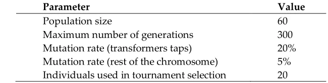
174
These constraints include voltage limits in load buses and transmission line loading as
175
indicated in equations (10) and (11). In this case, and are the voltage magnitude the ith bus
176
and apparent power flow in line li, respectively.
177
178
≤ ≤ , = 1, … , (10)
≤ , = 1, … , (11)
3. Implemented Genetic Algorithm
179
Genetic Algorithms are inspired by the mechanisms of natural evolution. They offer an
180
adaptive search based on the Darwinian principle of reproduction and survival of individuals that
181
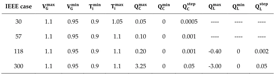
best adapt themselves to environmental conditions. These algorithms have been successfully
182
applied in optimization problems of great complexity as shown in [54]–[57]. The application of basic
183
principles of genetics to mathematical optimization begins with the random or pseudo-random
184
generation of an initial set of solutions (population). The algorithm starts by reading system data
185
and defining the codification of solutions (chromosome). As it will be explained later, the
186
codification was envisaged to take into account real power systems. Then, the SGA parameters are
187
set and an initial population is generated. In this case, it is guaranteed that all candidate solutions are
188
feasible (all control variables are within specified limits). Each individual must be read and decoded
189
by the algorithm indicating the set points of control variables (voltage of generators, transformer
190
taps, capacitors and reactor banks). With this information a power flow is run and power losses are
191
computed. After that, the operators of the SGA are applied (selection, crossover and mutation) until
192
a stopping criterion is met. Further details of the different stages regarding the SGA are explained
193
below. Figure 1 depicts the flowchart of the implemented SGA.
196
Figure 1. Flowchart of the implemented SGA
197
198
3.1 Codification
199
Codification of candidate solutions is a key aspect in the implementation of a GA. The
200
codification indicates how a candidate solution is represented, and it can facilitate or complicate the
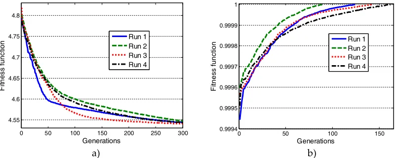
201
implementation of the GA’s operators. The proposed codification was devised to be suitable for real
202
power systems. Transformers taps as well as capacitor and reactor banks are discretized based on
203
system data when this one is available or using default parameters when it is not. Figure 2 illustrates
204
the representation of a potential solution to the ORPD problem. It consists of a vector with the
205
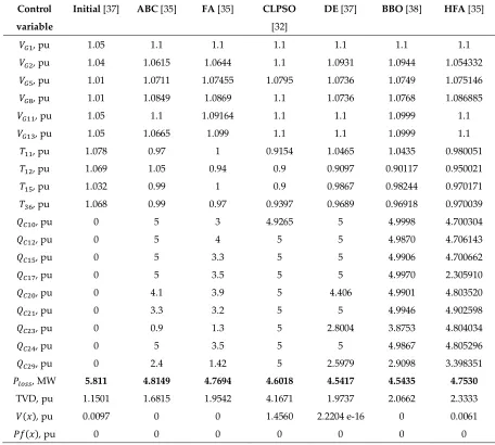
discretization of all control variables. Such variables are the setpoints of generators, transformers
206
taps and reactive power injections (from both capacitors and reactors). Control variables are
207
discretized as follows:
208
Voltage setpoints of generators are in a typical range of [0.95, 1.1] p.u, coded between discrete
209
values in the range [-100, 100]. However, any other range limit can be considered (depending
210
on specific system data). Reactive power limits of generators are considered within the power
211
flow subroutine.
212
Each capacitor is coded using the limits and step size reported for each power system test
213
case. The number of steps for a given capacitor bank is computed using its capacity and step
214
size (if provided). In this way, each capacitor might be coded differently. For example, in the
215
IEEE 30 bus test system all capacitor banks have a maximum capacity of 5 MW; however, the
step size is not provided in the original data; in this case, the step was set by default at 0.05
217
MVAR.
218
Transformers taps vary within the range [ , ] that may be different for every
219
transformer. If the limits of the tap setting and step size are provided in the system data, this
220
information is used in the codification. The number of steps is calculated as the integer
221
number that results from dividing the tap settings range ( − ) by the step size;
222
otherwise, a default range of [-10, 10] with steps of 1% is considered.
223
224
225
Figure 2. Codification of the implemented GA
226
227
Note that the codification of solutions was deviced in such a way that all control variables are
228
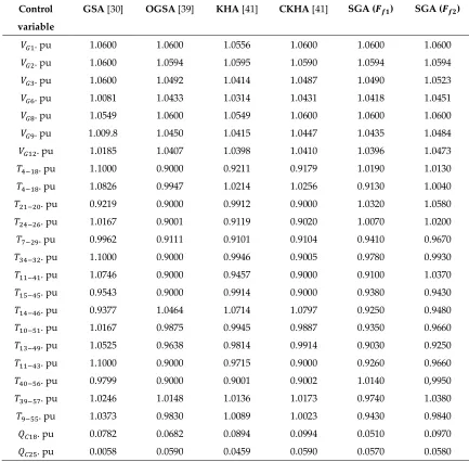
kept within their limits. A more accurate discretization is also possible; nevertheless, this might not
229
represent attainable solutions in real life. For example, capacitor and reactor banks can be coded to
230
represent variations in the range of few VARs; however, in real power systems these elements work
231
in the range of kVARs. On the other hand, given the fact that voltage is a continuous variable, a
232
fine-grain discretization of voltage magnitudes would represent solutions that are attainable in real
233
life. An advantage of a discrete codification is the fact that the range and number of steps can be
234
modified to adjust the particularities of the type of element that it represents. Steps of different sizes
235
can be used for transformer taps, reactors and capacitors.
236
237
3.2 GA Operators
238
Initial population is randomly generated within the specified limits of each control variable.
239
This is done to guarantee feasible candidate solutions. Afther that, the corresponding fitness
240
function of each candidate solution is evaluated. In order to compute power losses, it is necessary to
241
decode and run a power flow for each candidate solution. This is done with the software Matpower
242
5.1 [58]. Once the fitness function of each candidate solution is calculated, the selection operator is
243
carried out. In this case, selection is performed by tournament method. A number of tournaments
244
equal to the number of candidate solutions is performed. In each tournament, a subset of k
245
individuals is randomly chosen from the current population and the best individual of such subset is
246
selected to participate in the recombination or crossover stage. This stage combines the information
247
of selected individuals in every subset of control variables (multipoint crossover); Figure 3 illustrates
248
this stage. Mutation rate is dynamic (starts with a high rate and decreases steadily in every
249
generation) and can be applied differently to every subset of control variables. For example, the
250
mutation rate is lower for the subset of capacitors than it is for the subset of transformers tap;
251
consequently, at the end of the evolution process, there is a greater probability of change in
252
transformers taps than in capacitor banks. In this case, the mutated element takes a random value
253
within its limits. This is done to conserve the feasibiliy of candidate solutions.
In every cycle or generation, the offpring replace the parents only if they represent solutions
255
with better fitness functions. The process of selection, crossover and mutation is repeated until the
256
SGA reaches a specific stopping criterion. Such stopping criterion is determined by a maximum
257
number of generations or when a target on fitness function has been achieved without any violation
258
of system constraints.
259
Parents
Offspring Recombination points
Voltage
Setpoints Capacitors Reactors
Transformers Taps
260
Figure 3. Recombination stage
261
262
3.3 Constraint handling approaches
263
Evolutionary algorithms usually perform unconstrained searches, and thus require additional
264
mechanisms to handle constraints. In the ORPD problem, equality constraints (3) and (4) are met
265
by the load flow solution while constraints on control variables can be handled directly in the
266
problem codification. The remaining constraints to be enforced are voltage magnitudes in load buses
267
and power flow limits in lines (security constraints given by (10) and (11)). These constraints are
268
commonly enforced by some sort of penalty function. Two penalty functions are explored in this
269
paper as detailed below.
270
271
3.3.1 Traditional penalty function approach
272
A penalty function guarantees constraint enforcement by penalizing deviations of candidate
273
solutions from the feasible region of the problem. There are different ways of forming a penalty
274
function and several versions of them have been applied in the ORPD problem as reported in [42],
275
[48]–[51]. For comparative purposes, the penalty function approach shown in equation (12) was
276
selected, which is named as (fitness function 1).
277
278
( ) = ( ) + ( ) + ( ) (12)
279
In this case, x is the general representation of the optimization variables. In (12) the second and
280
third terms correspond to the traditional penalty function approach, where ( ) and ( )
281
represent constraint violations on voltage magnitudes in buses and power flows in lines,
282
respectively. and are penalty constants. Both ( ) and ( ) are sub-functions that
283
represent the distance to the feasible region of the problem; each of these are expressed in general
284
form as ( ) in equation (13).
286
( ) = 0, − + 0, ( − ) (13)
287
Where , and represent the optimization variables and their operational limits,
288
respectively. The fitness function used here primarily aims to control the voltage profile and power
289
flow limits. However, it can also be used to handle constraints on other variables such as voltage
290
levels of particular nodes (which cannot operate within conventional ranges), lines with special load
291
capability, etc. Note that ( ) is an alternative way of representing TVD. In this case, this
292
expression considers the fact that voltages operate within a given range and are not compared to a
293
fixed reference.
294
295
3.3.2 Alternative constraint handling approach
296
An alternative handling approach is based on the fitness function shown in equation (14),
297
named as (fitness function 2). This function is an adaptation of the one proposed in [59] which
298
was first introduced in the context of expansion planning for congestion management. In this case,
299
( ), ( ) and represent sub-functions for voltage magnitude in load bus i, power flow in
300
line j and power losses assessment, respectively. Figure 4 depicts the sub-functions under
301
consideration. Note that allows the planner to set a goal on power loss minimization. In this
302
case, it is assumed that the system operator has a reasonable estimation of the network power losses.
303
Also note that if all quantities are given in per unit, the maximum value of is equal to one,
304
independently of the number of constraints. This represents an advantage over traditional penalty
305
functions since it allows the algorithm to stop when the optimal solution (previously selected by the
306
planner) is achieved. It also allows to quickly asses the quality of a given solution which is given by
307
how close is to its maximum value. This way, the verification of both feasibility and optimality
308
of candidate solutions is straightforward.
309
310
= ( ) ( ) (14)
312
Figure 4. Sub-functions for: a) voltages in load buses, b) power flows in lines and c) active power losses
313
314
The mathematical expressions for the sub-functions depicted in figure 4 are given by (15)-(17).
315
316
( ) = ( ), ( ) (15)
( ) = ( ) (16)
= ( ) (17)
317
Where and are the maximum and minimum voltage limit on node i,
318
respectively; and are the maximum power flow limit on line j and its actual
319
value, respectively, and represents the goal on system real power losses which is compared
320
to actual power losses . The lambdas in every sub-function determine the hardness of the
321
constraint. Smaller values of lambda indicate softer constraints (see Figure 5).
322
Note that within sub-function ( ) and ( ) it is possible to set specific voltage limits per
323
node and specific power flow limits per line. This characteristic allows to define nodes and lines
324
with special limits for the ORPD problem.
325
326
a) b)
327
Figure 5. Sub-functions for: a) voltages in load buses and b) power flows in lines, for different lambdas
328
0 0.5 1 1.5 2
0 0.2 0.4 0.6 0.8 1
Voltage (p.u.)
F
it
n
e
s
s
= 1
= 10 = 5
= 0.5
0 0.5 1 1.5 2
0 0.2 0.4 0.6 0.8 1
Real power (p.u.)
F
itn
e
s
s
= 0.5
= 1
= 5
329
4. Tests and Results
330
To show the applicability of the proposed approach several tests were performed on the IEEE
331
30, 57, 118 and 300 bus test systems. Specialized literature regarding the ORPD problem usually
332
reports solutions on IEEE 30, 57 and 118 bus test systems. Also, several tests were performed using
333
the IEEE 300 bus test system with the aim of providing solutions for comparative purposes in later
334
works. All tests were carried out on a personal computer with Intel Core i7 (Quadcore) processor of
335
3.6 GHz and 8 GB of RAM memory. Test system data can be consulted in [37], [60], [61]. Active and
336
reactive power generation limits as well as active generator settings (except for the swing generator)
337
are taken from [61]. A summary of the test systems data is presented in Table 1.
338
339
Table 1. Main characteristics of the test systems under study.
340
Characteristic IEEE 30 IEEE 57 IEEE 118 IEEE 300
# buses 30 57 118 300
# load buses 24 50 64 231
# generators 6 7 54 69
# transformers 4 15 9 107
# capacitors 9 3 12 8
# reactors 0 0 2 6
# branches 41 80 186 411
# Control variables 19 25 77 190
Base case Ploss (MW) 5.833 27.864 132.863 408.316
Base case TVD (p.u) 0.58217 1.23358 1.439337 5.4286
341
4.1 Input parameters
342
Parameters of the SGA used for all simulations are described in Table 2. For simplicity
343
purposes, these set of parameters were tuned to be used with all tests systems. As regards fitness
344
function 2, it is necessary to set a goal on power losses for every test system. Such goal must be set by
345
the system planner taking into account the particularities of the network. An ambitious goal on
346
power loss reduction might result in unfeasible solutions while a conservative one might result in
347
sub-optimal solutions. Different goals on power loss reduction were tested and those that resulted in
348
feasible solutions are reported in Table 3. Note that for fitness function 1 there is no need of setting a
349
specific goal on power losses; since in this case, the algorithm always aims at minimizing losses even
350
at the expense of not fully enforcing security constraints. For both fitness functions voltage limits on
351
load buses were set as = 1.1 and = 0.9, and are 10000 and 1000, respectively.
352
Lambdas for fitness function 2 are: = 0.1, = 0.05, = 0.1.
353
354
Table 2. Genetic Algorithm parameters.
355
Parameter Value
Population size 60
Maximum number of generations 300
Mutation rate (transformers taps) 20%
Mutation rate (rest of the chromosome) 5% Individuals used in tournament selection 20
356
Table 3. Goals on system power losses for fitness function 2
357
IEEE case Current power
losses (MW)
Goal on system power losses
(% Total Gen) (MW)
30 5.833 1.58 4.57
57 27.864 2.55 23.69
358
Maximum and minimum limits of control variables for the IEEE test cases, with a base of 100
359
MVA, are given in the Table 4 [37], [60], [61]. Note that the main differences among these cases are
360
maximum limits of capacitor banks and reactors.
361
362
Table 4. Limits of control variables for different IEEE cases (p.u)
363
IEEE case
30 1.1 0.95 0.9 1.05 0.05 0 0.0005 ---- ---- ----
57 1.1 0.95 0.9 1.1 0.10 0 0.001 ---- ---- ----
118 1.1 0.95 0.9 1.1 0.20 0 0.001 -0.40 0 0.002
300 1.1 0.95 0.9 1.1 3.25 0 0.05 -3.00 0 0.05
364
4.2 Results with the IEEE 30 bus power system
365
The IEEE 30 bus power system comprises nineteen control variables: six generator voltage
366
magnitudes (at buses 1, 2, 5, 8, 11 and 13), four tap changing transformers (at branches 6–9, 6–10, 4–
367
12 and 28–27) and nine shunt capacitor devices (at buses 10, 12, 15,17, 20, 21, 23, 24 and 29). The total
368
system demand is 283.4 MW [37], [60], [61]. As it is well known, power losses are greatly affected by
369
maximum voltage limits of generators. Allowing higher voltage limits results in lower power losses
370
and vice versa. Regarding the IEEE 30 bus power system, some studies consider upper voltage limits
371
of 1.1 p.u while some others consider 1.05 p.u. In this case, several tests were performed considering
372
both limits, for comparative purposes. Table 5a and Table 5b present the comparison of results when
373
the upper voltage limit of generators is set to 1.1 p.u. In this case, ABC and HFA stand for artificial
374
bee colony and hybrid firefly algorithm, respectively. The solutions obtained with the proposed
375
methodology, using and , are presented in the last two columns of Table 5b. Power losses
376
and total voltage deviation (TVD) given by equations (1) and (2), respectively, are computed for
377
other metaheuristics using the reported values of control variables with the software Matpower 5.1
378
[58]. Also ( ) and ( ) are computed as given by equation (13). Note that both expressions
379
represent the distance to the feasible region for voltage and power low limits, respectively. Power
380
losses obtained with the proposed SGA were 4.5399 MW and 4.5692 MW with total voltage
381
deviations of 2.0105 p.u and 1.8333 p.u for and , respectively. However, both ( ) and
382
( ) are zero, which indicates that the solution found by the SGA guarantees the operation of the
383
system within feasible ranges. When the SGA is implemented with it obtains lower power losses
384
but higher voltage deviations. Note that the SGA outperforms other metaheuristic techniques
385
reported in Table 5a and Table 5b when using ; however, DE, MFO and BBO obtain slightly
386
better results (with less than 1% of difference) than the proposed methodology when applying .
387
Table 5c presents the comparison of results when the upper voltage limit of generators is set to 1.05
388
p.u. In this case, ALC-PSO stands for particle swarm optimization with an aging leader and
389
challengers. Power losses obtained with the proposed SGA were 5.072 MW using both objective
390
functions. As expected, power losses in this case are higher than those obtained considering higher
391
voltage limits (see Table 5a and Table 5b). Nevertheless, the proposed SGA was able to obtain better
392
solutions than those obtained with other metaheuristics. Figure 6 depicts the convergence of the
393
algorithm for both objective functions for four independent runs (considering 1.1 p.u as voltage limit
394
of generators). Note that when using the algorithm requires fewer generations to reach
395
convergence, which has a positive impact in computational time.
396
397
398
399
400
401
Table 5a. Best control variable settings reported for power loss minimization of the IEEE 30 bus test system
402
with different algorithms considering 1.1 p.u as the maximum setpoints of generators.
403
Control
variable
Initial [37] ABC [35] FA [35] CLPSO
[32]
DE [37] BBO [38] HFA [35]
, pu 1.05 1.1 1.1 1.1 1.1 1.1 1.1
, pu 1.04 1.0615 1.0644 1.1 1.0931 1.0944 1.054332
, pu 1.01 1.0711 1.07455 1.0795 1.0736 1.0749 1.075146
, pu 1.01 1.0849 1.0869 1.1 1.0736 1.0768 1.086885
, pu 1.05 1.1 1.09164 1.1 1.1 1.0999 1.1
, pu 1.05 1.0665 1.099 1.1 1.1 1.0999 1.1
, pu 1.078 0.97 1 0.9154 1.0465 1.0435 0.980051
, pu 1.069 1.05 0.94 0.9 0.9097 0.90117 0.950021
, pu 1.032 0.99 1 0.9 0.9867 0.98244 0.970171
, pu 1.068 0.99 0.97 0.9397 0.9689 0.96918 0.970039
, pu 0 5 3 4.9265 5 4.9998 4.700304
, pu 0 5 4 5 5 4.9870 4.706143
, pu 0 5 3.3 5 5 4.9906 4.700662
, pu 0 5 3.5 5 5 4.9970 2.305910
, pu 0 4.1 3.9 5 4.406 4.9901 4.803520
, pu 0 3.3 3.2 5 5 4.9946 4.902598
, pu 0 0.9 1.3 5 2.8004 3.8753 4.804034
, pu 0 5 3.5 5 5 4.9867 4.805296
, pu 0 2.4 1.42 5 2.5979 2.9098 3.398351
, MW 5.811 4.8149 4.7694 4.6018 4.5417 4.5435 4.7530
TVD, pu 1.1501 1.6815 1.9542 4.1671 1.9737 2.0662 2.3333
( ), pu 0.0097 0 0 1.4560 2.2204 e-16 0 0.0061
( ), pu 0 0 0 0 0 0 0
404
Table 5b. Best control variable settings reported for power loss minimization of the IEEE 30 bus test system
405
with different algorithms considering 1.1 p.u as the maximum setpoints of generators.
406
Control
variable
GSA [30] MFO [26] IGSA-CSS
[31]
FAHLCPSO
[33]
SGA ( ) SGA ( )
. pu 1.071652 1.1000 1.081281 1.1000 1.1000 1.1000
. pu 1.022199 1.0943 1.072177 1.0387 1.0940 1.0970
. pu 1.040094 1.0747 1.050142 1.0161 1.0745 1.0805
. pu 1.050721 1.0766 1.050234 1.0290 1.0767 1.0835
. pu 0.977122 1.1000 1.100000 1.0123 1.1000 1.1000
. pu 0.967650 1.1000 1.068826 1.1000 1.1000 1.1000
. pu 1.098450 1.0433 1.0800 1.0223 1.0510 1.0680
. pu 0.982481 0.9000 0.9020 0.9107 0.9000 0.9080
. pu 1.095909 0.97912 0.9900 1.0098 0.9830 0.9990
. pu 1.059339 0.96474 0.9760 0.9744 0.9670 0.9750
. pu 4.372261 0.0500 0.0000 0.0500 0.0500 0.0235
. pu 0.119957 0.048055 0.0380 0.020981 0.0500 0.0445
. pu 2.087617 0.0500 0.0490 0.0500 0.0500 0.0480
. pu 0.357729 0.040263 0.0395 0.035512 0.0435 0.0290
. pu 0.260254 0.0500 0.0500 0.040005 0.0500 0.0455
. pu 0.000000 2.5193 0.0275 0.031928 0.0270 0.0370
. pu 1.383953 0.0500 0.0500 0.048800 0.0500 0.0465
. pu 0.000317 0.021925 0.0240 0.021000 0.0240 0.0135
. MW 5.5372 4.5410 4.7620 6.8230 4.5399 4.5692
TDV. pu 1.6552 2.0316 1.1487 0.7914 2.0105 1.8333
( ), pu 0 0 0 0 0 0
( ), pu 0 0 0 0 0 0
407
Table 5c. Best control variable settings reported for power loss minimization of the IEEE 30 bus test system with
408
different algorithms considering 1.05 p.u as the maximum setpoints of generators.
409
Control
variable
OGSA [39] ALC-PSO
[53]
KHA [41] CKHA
[41]
NGBWCA
[34]
SGA ( ) SGA ( )
. pu 1.0500 1.0500 1.0500 1.0500 1.0502 1.0500 1.0500
. pu 1.0410 1.0384 1.0381 1.0473 1.0382 1.0445 1.0445
. pu 1.0154 1.0108 1.0110 1.0293 1.0107 1.0245 1,0240
. pu 1.0267 1.0210 1.0250 1.0350 1.0212 1.0265 1,0260
. pu 1.0082 1.0500 1.0500 1.0500 1.0503 1.0500 1,0500
. pu 1.0500 1.0500 1.0500 1.0500 1.0500 1.0500 1,0500
. pu 1.0585 0.9521 0.9541 0.9916 0.9520 1.0500 1,0490
. pu 0.9089 1.0299 1.0412 0.9538 1.0295 0.9000 0,9000
. pu 1.0141 0.9721 0.9514 0.9603 0.9720 0.9880 0,9880
. pu 1.0182 0.9657 0.9541 0.9670 0.9661 0.9660 0,9650
. pu 0.0330 0.0090 0.0089 0.0092 0.0097 0.0500 0.0500
. pu 0.0249 0.0126 0.0000 0.0000 0.0125 0.0500 0.0500
. pu 0.0177 0.0209 0.0141 0.0153 0.0212 0.0500 0.0500
. pu 0.0500 0.0500 0.04989 0.0497 0.0541 0.0500 0.0500
. pu 0.0334 0.0031 0.0314 0.0302 0.0043 0.0500 0.0500
. pu 0.0403 0.0293 0.0345 0.0500 0.0289 0.0500 0.0500
. pu 0.0269 0.0226 0.0241 0.0134 0.0229 0.0360 0.0360
. pu 0.0500 0.0500 0.0500 0.0500 0.0498 0.0500 0.0500
. pu 0.0194 0.0107 0.0107 0.0121 0.0106 0.0280 0.0275
. MW 5.5192 5.4711 5.5407 5.4285 5.4720 5.0272 5.0272
TDV. pu 0.8540 0.3001 0.2963 0.3524 0.3003 0.7369 0.7372
( ), pu 0 0 0 0 5e-4 0 0
( ), pu 0 0 0 0 0 0 0
411
a) b)
412
Figure 6. Convergence curves for a) and b) considering four independent runs (IEEE 30 bus power
413
system).
414
415
4.3 Results with the IEEE 57 bus power system.
416
The IEEE 57 bus power system consists of eighty branches (lines and transformers), seven
417
generators, fifteen transformers (available for tap changing), and three shunt capacitor devices (at
418
buses 18, 25 and 53). The total system demand is 1250.8 MW [61]. A comparison of the best solutions
419
found with different metaheuristics for the ORPD problem applied to this power system is reported
420
in Table 6a and Table 6b with a base of 100 MVA. In this case, the maximum voltage limit of
421
generators was set to 1.06 p.u for comparative purposes. Power losses, voltage deviations, as well as
422
( ) and ( ) were computed for other metaheuristics using the reported values of control
423
variables. Note that the proposed SGA was able to obtain better results than the other
424
metaheuristics, especially when using ; however, at a expense of higher TVD. Furthermore, the
425
values obtained with the SGA for ( ) and ( ) are approximately zero, meaning that the
426
solution found meets the operational constraints defined for this system, which is not always the
427
case for the other reported metaheuristics. Figure 7 depicts the convergence of the algorithm for both
428
objective functions considering four independent runs. Note that fewer generations are required to
429
reach optimality when is implemented.
430
431
Table 6a. Best control variable settings for power loss minimization of IEEE 57 bus test system with different
432
algorithms.433
Control variable Initial [37] SOA [28] CLPSO [30]DE [28] BBO [30] ALC-PSO
[53]
MFO [26] NGBWCA
[34]
. pu 1.0400 1.0541 1.0541 1.0397 1.0600 1.0600 1.06000 1.0600
. pu 1.0100 1.0529 1.0529 1.0463 1.0504 1.0593 1.05870 1.0591
. pu 0.9850 1.0337 1.0337 1.0511 1.0440 1.0491 1.04690 1.0492
. pu 0.9800 1.0313 1.0313 1.0236 1.0376 1.0432 1.04210 1.0399
. pu 1.0500 1.0496 1.0496 1.0538 1.0550 1.0600 1.06000 1.0586
. pu 0.9800 1.0302 1.0302 0.9451 1.0229 1.0451 1.04230 1.0461
. pu 1.0150 1.0302 1.0342 0.9907 1.0323 1.0411 1.03730 1.0413
. pu 0.9700 0.9900 0.9900 1.0200 0.9669 0.9611 0.95011 0.9712
. pu 0.9780 0.9800 0.9800 0.9100 0.9902 0.9109 1.00760 0.9243
. pu 1.0430 0.9900 0.9900 0.9700 1.0120 0.9000 1.00630 0.9123
. pu 1.0430 1.0100 1.0100 0.9100 1.0087 0.9004 1.00760 0.9001
. pu 0.9670 0.9900 0.9900 0.9600 0.9707 0.9106 0.97523 0.9112
. pu 0.9650 0.9300 0.9300 0.9900 0.9686 0.9000 0.97218 0.9004
. pu 0.9550 0.9100 0.9100 0.9800 0.9008 0.9000 0.90000 0.9128
0 50 100 150 200 250 300
4.55 4.6 4.65 4.7 4.75 4.8 Generations F it n e s s f u n c ti o
n Run 1
Run 2 Run 3 Run 4
0 50 100 150
0.9994 0.9995 0.9996 0.9997 0.9998 0.9999 1 Generations F it n e s s f u n c ti o
n Run 1
. pu 0.9550 0.9700 0.9700 0.9600 0.9660 0.9000 0.97186 0.9000
. pu 0.9000 0.9500 0.9500 1.0500 0.9507 1.0275 0.95355 1.0218
. pu 0.9300 0.9800 0.9800 1.0700 0.9641 0.9876 0.96736 0.9902
. pu 0.8950 0.9500 0.9500 0.9900 0.9246 0.9756 0.92788 0.9568
. pu 0.9580 0.9500 0.9500 1.0600 0.9502 0.9000 0.96406 0.9000
. pu 0.9580 1.0000 1.0000 0.9900 0.9966 0.9000 0.99980 0.9000
. pu 0.9800 0.9600 0.9600 0.9700 0.9628 1.0121 0.96060 1.0118
. pu 0.9400 0.9700 0.9700 1.0700 0.9600 0.9944 0.97899 1.0000
. pu 0 0.0988 0.0988 0 0.09782 0.0994 0.099968 0.0914
. pu 0 0.0542 0.0542 0 0.05899 0.0590 0.05900 0.0587
. pu 0 0.0628 0.0628 0 0.06289 0.0630 0.06300 0.0634
. pu 0.2786 0.2487 0.2489 0.3594 0.2454 0.2618 0.242529 0.2674
TDV. pu 4.1788 1.0775 1.0929 4.1788 1.3548 2.2077 1.4885 2.1427
( ), pu 0.7951 0 0 0.7951 0 0.1428 7.29e-5 0.3913
( ), pu 0.2948 0.0035 0.0022 0.2948 3.4900e-04 0.0829 0 0.0895
434
Table 6b. Best control variable settings for power loss minimization of IEEE 57 bus test system with different
435
algorithms
436
Control
variable
GSA [30] OGSA [39] KHA [41] CKHA [41] SGA ( ) SGA ( )
. pu 1.0600 1.0600 1.0556 1.0600 1.0600 1.0600
. pu 1.0600 1.0594 1.0595 1.0590 1.0594 1.0594
. pu 1.0600 1.0492 1.0414 1.0487 1.0490 1.0523
. pu 1.0081 1.0433 1.0314 1.0431 1.0418 1.0451
. pu 1.0549 1.0600 1.0549 1.0600 1.0600 1.0600
. pu 1.009.8 1.0450 1.0415 1.0447 1.0435 1.0484
. pu 1.0185 1.0407 1.0398 1.0410 1.0396 1.0473
. pu 1.1000 0.9000 0.9211 0.9179 1.0190 1.0130
. pu 1.0826 0.9947 1.0214 1.0256 0.9130 1.0040
. pu 0.9219 0.9000 0.9912 0.9000 1.0320 1.0580
. pu 1.0167 0.9001 0.9119 0.9020 1.0070 1.0200
. pu 0.9962 0.9111 0.9101 0.9104 0.9410 0.9670
. pu 1.1000 0.9000 0.9946 0.9005 0.9780 0.9930
. pu 1.0746 0.9000 0.9457 0.9000 0.9100 1.0370
. pu 0.9543 0.9000 0.9914 0.9000 0.9380 0.9430
. pu 0.9377 1.0464 1.0714 1.0797 0.9250 0.9480
. pu 1.0167 0.9875 0.9945 0.9887 0.9350 0.9660
. pu 1.0525 0.9638 0.9814 0.9914 0.9030 0.9250
. pu 1.1000 0.9000 0.9715 0.9000 0.9260 0.9660
. pu 0.9799 0.9000 0.9001 0.9002 1.0140 0,9950
. pu 1.0246 1.0148 1.0136 1.0173 0.9740 1.0380
. pu 1.0373 0.9830 1.0089 1.0023 0.9430 0.9840
. pu 0.0782 0.0682 0.0894 0.0994 0.0510 0.0970
. pu 0.0468 0.0630 0.0625 0.0630 0.0630 0.0435
. pu 0.2940 0.2642 0.2618 0.2748 0.23836 0.24325
TDV. pu 2.8536 2.1764 2.4490 2.2741 2.7021 1.7616
( ), pu 0.4369 0.1036 0.0851 0.0818 0 0
( ), pu 0.0483 0.0948 0.0107 0.1445 9.9e-7 0
437
438
a) b)
439
Figure 7. Convergence curves for a) and b) considering four independent runs (IEEE 57 bus power
440
system).
441
442
4.4 Results with the IEEE 118 bus power system.
443
The IEEE 118 bus test system has seventy-seven control variables; these consist of fifty-four
444
generator buses, nine tap changing transformers, twelve capacitor devices and two reactor devices.
445
The total system demand is 4242 MW [61]. The optimal settings of control variables are presented in
446
Table 7a and Table 7b; power losses, voltage deviations, ( ) and ( ) were computed for other
447
metaheuristics using the reported values of control variables. In this case, power losses are given
448
with a base of 100 MVA. Note that the solutions obtained with the proposed approach are better
449
than those reported with other metaheuristics. Furthermore, the values obtained with the SGA for
450
( ) and ( ) are zero, which means that the solution found meets all operational constraints.
451
Figure 8 depicts the convergence of the algorithm for both objective functions considering four
452
independent runs. Note that in general fewer generations are needed to reach optimality when using
453
.
454
455
Table 7a. Best control variable settings for power loss minimization of IEEE 118 bus test system with different
456
algorithms457
Control variable MFO [26] NGBWCA [34] FAHCLPSO [33] Control variable MFO [26] NGBWCA [34] FAHCLPSO [33]. pu 1.0173 1.0215 1.0120 . pu 1.0496 0.9989 1.0298
pu 1.0402 1.0431 1.0523 . pu 1.0600 1.0001 1.1005
. Pu 1.0292 1.0312 1.0666 . pu 1.0551 1.0467 1.0498
. pu 1.0600 1.0539 1.0597 . pu 1.0584 1.0213 1.0565
. pu 1.0374 1.0271 1.0725 . pu 1.0442 1.0416 1.0413
. pu 1.0250 1.0316 1.0333 . pu 1.0333 1.0174 1.0189
. pu 1.0268 1.0129 1.0012 . pu 1.0281 1.0223 1.1000
. pu 1.0298 1.0075 1.0058 . pu 1.0161 1.0340 1.0222
. pu 1.0275 1.0102 1.1000 . pu 1.0215 1.0103 1.0115
. pu 1.0483 1.0208 1.0971 . pu 1.0280 1.0345 1.1000
0 50 100 150 200 250 300
24 24.5 25 25.5 26 Generations F it n e s s f u n c ti o n Run 1 Run 2 Run 3 Run 4
. pu 1.0600 1.0531 1.0899 . pu 1.0042 1.0160 1.0500
. pu 1.0600 0.9941 1.1000 . pu 1.0350 1.0181 1.0099
. pu 1.0267 1.0291 1.0654 . pu 1.0484 1.0330 1.0500
. pu 1.0101 1.0275 1.0318 . pu 1.01360 1.0051 1.0214
. pu 1.0226 1.0201 1.0322 . pu 1.10000 0.9614 1.0533
. pu 1.0556 1.0014 0.9999 . pu 1.00380 0.9961 1.0555
. pu 1.0548 1.0412 0.9998 . pu 0.98263 0.9523 0.9995
. pu 1.0419 1.0400 1.0501 . pu 0.98430 1.0521 1.0619
. pu 1.0429 1.0512 1.0231 . pu 1.01390 0.9520 1.0318
. pu 1.0450 1.0170 1.0005 . pu 1.10000 0.9812 1.0490
. pu 1.0589 1.0510 0.9897 . pu 1.10000 0.9510 0.9660
. pu 1.0284 1.0392 0.9998 . pu 0.96831 0.9754 0.9732
. pu 1.0289 1.0331 1.0222 . pu 0 −0.0723 0.0035
. pu 1.0283 1.0372 1.0008 . pu 0 0.0483 0.101922
. pu 1.0512 1.0564 1.0731 . pu −0.03126 −0.2390 0.017500
. pu 1.0534 1.0565 1.0258 . pu 0.10 0.0032 0.04400
. pu 1.0506 1.0489 1.0059 . pu 0 0.0372 0.069894
. pu 1.0596 1.0435 1.0630 . pu 0 0.0624 0.071289
. pu 1.0600 1.0435 1.0312 . pu 0.000842 0.0172 0.066668
. pu 1.0600 1.0489 1.0636 . pu 0.022054 0.0013 0.110952
. pu 1.0600 1.0113 1.1000 . pu 0.20 0.0621 0.15000
. pu 1.0526 1.0382 1.0500 . pu 0 0.0463 0.105509
. pu 1.0600 0.9926 1.0981 . pu 0.10 0.0560 0.055540
. pu 1.0600 0.9934 1.0444 . pu 0 0.0653 0.151895
. pu 1.0390 1.0324 1.0037 . pu 0.06 0.0072 0.044140
. pu 1.0502 1.0185 1.0559 . pu 0.06 0.0108 0.022310
. pu 1.0600 1.0021 0.9999 . pu 1.164254 1.2147 1.162479
. pu 1.0600 1.0312 1.0882 TDV. pu 2.3416 1.452 2.5204
. pu 1.0599 1.0212 1.0303 ( ), pu 0 0 0
. pu 1.0600 1.0387 1.0001 ( ),pu 0 0 0
. pu 1.0431 1.0071 1.0018
458
Table 7b. Best control variable settings for power loss minimization of IEEE 118 bus test system with different
459
algorithms
460
Control
variable
ALC-PSO
[53]
GSA
[30]
SGA
( )
SGA
( )
Control
variable
ALC-PSO
[53]
GSA
[30]
SGA
( )
SGA
( )
. pu 1.0218 0.9600 1.0880 1.0947 . pu 0.9997 1.0032 1.0955 1.0985
pu 1.0432 0.9620 1.1000 1.1000 . pu 1.0012 1.0927 1.0993 1.0992
. Pu 1.0224 0.9729 1.0963 1.0970 . pu 1.0481 1.0433 1.0955 1.0992
. pu 1.0543 1.0570 1.0828 1.0820 . pu 1.0332 1.0786 1.1000 1.1000
. pu 1.0901 1.0885 1.0910 1.0895 . pu 1.0422 1.0266 1.0993 1.0985
. pu 1.0325 0.9630 1.0940 1.0992 . pu 1.0183 0.9808 1.0963 1.1000
. pu 1.0140 1.0127 1.0850 1.0955 . pu 1.0226 1.0163 1.0948 1.0985
. pu 1.0104 1.0003 1.0850 1.0992 . pu 1.0349 1.0218 1.0963 1.1000
. pu 1.0200 1.0105 1.0978 1.0985 . pu 1.0425 0.9852 1.1000 1.0977
. pu 1.0551 1.0102 1.1000 1.1000 . pu 1.0162 0.9500 1.0835 1.0985
. pu 0.9932 1.0401 1.1000 1.0992 . pu 1.0188 0.9764 1.0963 1.0977
. pu 1.0288 0.9809 1.0933 1.0977 . pu 1.0331 1.0372 1.0985 1.0992
. pu 1.0288 0.9500 1.0888 1.0977 . pu 1.0065 1.0659 0.9920 1.0000
. pu 1.0248 0.9552 1.0895 1.0970 . pu 0.9617 0.9534 1.0450 1.0110
. pu 1.0362 0.9910 1.0940 1.0887 . pu 0.9745 0.9328 0.9870 1.0050
. pu 1.0407 1.0091 1.0940 1.0925 . pu 0.9404 1.0884 0.9790 0.9500
. pu 1.0391 0.9505 1.0843 1.0955 . pu 1.0531 1.0579 0.9800 0.9550
. pu 1.0507 0.9500 1.0873 1.0985 . pu 0.9539 0.9493 1.0040 0.9990
. pu 1.0171 0.9814 1.0903 1.1000 . pu 0.9448 0.9975 0.9960 1.0730
. pu 1.0492 1.0444 1.1000 1.1000 . pu 0.9502 0.9887 0.9600 0.9720
. pu 1.0424 1.0379 1.0903 1.0992 . pu 0.9747 0.9801 0.9840 0.9800
. pu 1.0339 0.9907 1.0903 1.0992 . pu -0.0075 0.0000 -0.0050 -0.0020
. pu 1.0393 1.0333 1.0888 1.0992 . pu 0.0677 0.0746 0.0500 0.0160
. pu 1.0585 1.0099 1.1000 1.1000 . pu -0.2399 0.0000 -0.0050 0.000
. pu 1.0569 1.0925 1.0993 1.0992 . pu 0.0038 0.0604 0.0145 0.0890
. pu 1.0491 1.0393 1.0948 1.0977 . pu 0.0179 0.0333 0.0025 0.0270
. pu 1.0437 0.9998 1.1000 1.0992 . pu 0.0780 0.0651 0.0155 0.0470
. pu 1.0716 1.0355 1.1000 1.0992 . pu 0.0789 0.0447 0.0350 0.0040
. pu 1.0535 1.1000 1.1000 1.1000 . pu 0.0000 0.0972 0.0005 0.1070
. pu 1.0111 1.0992 1.0880 1.0985 . pu 0.0717 0.1425 0.0190 0.0220
. pu 1.0389 1.0014 1.0955 1.1000 . pu 0.0589 0.1749 0.0470 0.0650
. pu 0.9932 1.0111 1.0955 1.0977 . pu 0.0561 0.0428 0.0025 0.0020
. pu 0.9912 1.0476 1.0775 1.0940 . pu 0.0641 0.1204 0.0005 0.1860
. pu 1.0335 1.0211 1.0768 1.0805 . pu 0.0000 0.0226 0.0380 0.0135
. pu 1.0191 1.0187 1.0895 1.09475 . pu 0.0110 0.0294 0.0130 0.0495
. pu 1.0247 1.0462 1.0993 1.1000 . pu 1.2153 1.2776 1.0633 1.0846
. pu 1.0324 1.0491 1.1000 1.0992 TDV. pu 1.4651 2.2243 5.5245 5.7253
. pu 1.0243 1.0426 1.0985 1.0970 ( ), pu 0 0 0 0
. pu 1.0303 1.0955 1.1000 1.1000 ( ), pu 0 0 0 0
. pu 1.0072 1.0417 1.0910 1.0985
461
462
0 50 100 150 200 250 300
100 200 300 400 500 600 700
Generations
F
itn
e
s
s
f
u
n
c
ti
o
n Run 1
Run 2 Run 3 Run 4
20 40 60 80 100 120
0.965 0.97 0.975 0.98 0.985 0.99 0.995 1
Generations
F
it
n
e
s
s
f
u
n
c
tio
n
a) b)
463
Figure 8. Convergence curves for a) and b) considering four independent runs (IEEE 118 bus power
464
system).
465
466
4.5 Results with the IEEE 300 bus power system.
467
The IEEE 300 bus test system has one hundred and ninety control variables. These consist of
468
sixty-nine generator buses, one hundred and seven tap changing transformers, eight capacitor
469
devices and six reactor devices. The total system demand is 23525.85 MW [49]. So far, no results for
470
the ORPD problem applied to this system have been reported in the specialized literature. The best
471
control variable settings obtained with the SGA are presented in Table 8. Power losses are given with
472
a base of 100 MVA and voltage limits on generators are set to 1.1 p.u. In this case, a reduction of 9.9
473
% in power losses is obtained when using . Also, note that the values of ( ) and ( ) are
474
approximately zero, which means that the solution found meets the operational constraints. The
475
solution reported in Table 8 can be used for further comparisons in future research. Figure 9
476
depicts the convergence of the algorithm for both objective functions considering four independent
477
runs. Note that as with the previous systems, the SGA reaches optimality with fewer generations
478
when is implemented.
479
480
Table 8. Best control variable settings for power loss minimization of IEEE 300 bus test system
481
Control
variable
Initial SGA
( )
SGA
( )
Control
variable
Initial SGA
( )
SGA
( )
Control
variable
Initial SGA
( )
SGA
( )
. pu 1.0522 1.0992 1.0977 . pu 1.0000 0.9380 1.0130 . pu 0.9284 0,9800 0.9320 . pu 1.0650 1.0992 1.0955 . pu 1.0000 1.0700 1.0880 . pu 1.0000 0,9970 0.9890 . pu 1.0650 1.0985 1.0940 . pu 1.0000 1.0290 1.0710 . pu 1.0000 0,9080 1.0890 . pu 1.0551 1.0857 1.0842 . pu 0.9583 1.0050 0.9980 . pu 1.0000 1,0530 0.9390 . pu 1.0435 1.1000 1.0970 . pu 1.0000 0.9760 0.9830 . pu 0.95 0,9320 1.0580 . pu 1.0150 1.0992 1.0955 . pu 1.0000 0.9620 1.0960 . pu 1.0000 1,0130 1.0740 . pu 1.0100 1.0992 1.0992 . pu 1.0000 1.0220 1.0270 . pu 1.0000 1.0000 1.0190 . pu 1.0080 1.0940 1.0947 . pu 1.0000 1.0830 1.0120 . pu 1.0000 1,0270 0.9540 . pu 1.0000 1.0970 1.0992 . pu 0.9470 1.0460 1.0240 . pu 1.0000 1,0110 0.9990 . pu 1.0500 1.0947 1.0962 . pu 0.9560 0.9400 0.9750 . pu 1.0000 1,0200 0.9930 . pu 1.0000 1.0992 1.1000 . pu 0.9710 0.9970 0.9550 . pu 1.0000 1,0020 1.0240 . pu 1.0400 1.0985 1.0662 . pu 0.9480 1.0150 1.0300 . pu 1.0000 0,9940 1.0130 . pu 1.0000 1.0947 1.0962 . pu 0.9590 1.0120 0.9620 . pu 1.0000 0,9770 0.9840 . pu 1.0165 1.0992 1.0985 . pu 1.0460 1.0840 1.0400 . pu 1.0000 0,9570 0.9880 . pu 1.0100 1.0985 1.0970 . pu 0.9850 1.0280 1.0640 . pu 0.9420 0,9900 1.0150 . pu 1.0000 1.1000 1.0992 . pu 0.9561 0.9790 0.9740 . pu 0.9650 0,9980 1.0660 . pu 1.0500 1.0992 1.0970 . pu 0.9710 0.9500 0.9210 . pu 0.9500 1,0420 1.0590 . pu 0.993 1.0962 1.0917 . pu 0.9520 0.9960 1.0370 . pu 0.9420 0,9740 0.9030 . pu 1.0100 1.0985 1.0985 . pu 0.9430 1.0620 0.9400 . pu 0.9420 0,9120 1.0650 . pu 1.0507 1.0985 1.0962 . pu 1.0100 0.9410 1.0530 . pu 0.95650 1,0350 1.0090 . pu 1.0507 1.0992 1.1000 . pu 1.0080 0.9770 1.0060 . pu 3.2500 1.8000 0.8000 . pu 1.0323 0.9897 1.0940 . pu 1.0000 0.9870 0.9850 . pu 0.5500 0.0200 0.4800 . pu 1.0145 1.1000 1.0962 . pu 0.9750 0.9550 1.0230 . pu 0.3450 0.0000 0.1250 . pu 1.0507 1.0955 1.0992 . pu 1.0170 0.9970 0.9810 . pu -2.120 -0.020 -1.740 . pu 1.0507 1.0985 1.0992 . pu 1.0000 1.0450 1.0820 . pu -1.030 0.0000 -0.060 . pu 1.0507 1.1000 1.0977 . pu 1.0000 1.0100 0.9690 . pu 0.5300 0.0900 0.1950 . pu 1.0290 1.0550 1.0977 . pu 1.0000 1.0040 0.9490 . pu 0.4500 0.1450 0.2500 . pu 1.0500 1.0977 1.0977 . pu 1.0000 1.0130 0.9480 . pu -1.5000 -0.060 -0.080 . pu 1.0145 1.0977 1.0977 . pu 1.0150 1.0000 1.0960 . pu -3.000 -0.350 -0.100 . pu 1.0507 1.0925 1.0977 . pu 0.9670 0.9810 1.0580 . pu -1.500 -0.080 -0.040 . pu 0.9967 1.0985 1.0977 . pu 1.0100 0.9140 0.9940 . pu -1.400 -0.260 -0.100 . pu 1.0212 1.0992 1.0985 . pu 1.0500 0.9540 1.0060 . pu 0.4560 0.1450 0.1250 . pu 1.0145 1.1000 1.0962 . pu 1.0000 1.0820 1.0250 . pu 0.0240 0.0120 0.0500 . pu 1.0017 1.0947 1.0970 . pu 1.0522 1.0140 1.0970 . pu 0.0172 0.0075 0.0475 . pu 0.9893 1.0992 1.1000 . pu 1.0522 1.0060 1.0290 . pu 4.0831 3.5710 3.6798 . pu 1.0507 1.1000 1.0985 . pu 1.0500 1.0480 1.0150 TDV. pu 5.4286 15.744 15.315 . pu 1.0507 1.0992 1.0992 . pu 0.9750 0.9910 1.0610 ( ), pu 0 4.77e-5 0
.pu 1.0145 1.0940 1.0962 . pu 1.0000 0.9180 0.9710 ( ), pu 0 0 0
. pu 0.9945 1.0962 1.0962 . pu 1.0350 1.0510 1.0040
483
a) b)
484
Figure 9. Convergence curves for a) and b) considering four independent runs (IEEE 300 bus power
485
system).
486
487
4.6 Comparison of fitness functions performance
488
Table 9 presents a statistical description of the results obtained with the SGA for all test cases
489
over one hundred runs. Note that using yields better results than using . The maximum
490
difference of both fitness functions regarding the reduction on power losses is about 2.66 %; but
491
significantly different on computation time. Faster results are obtained when using . For the IEEE
492
300 bus test system the reduction on computation time is about 21.25%; however, for the IEEE 57 bus
493
test system this reduction is about 90.37%. This advantage is due to the fact that using allows a
494
straightforward verification of both feasibility and optimality. Consequently, the SGA can stop the
495
process when the optimal solution is found even if the maximum number of iterations has not been
496
reached.
497
The standard deviations results using are smaller than those obtained using ; this means
498
that the reproducibility of results is higher when the SGA uses . On the other hand, success rate is
499
an indicator of the percentage of runs in which a feasible operational point is obtained before the
500
SGA reaches the maximum number of generations (number of times the algorithm obtains feasible
501
optimal solutions). For example, the last column in Table 9 indicates that in 97 of the 100 runs
502
reaches its optimal value before completing the maximum of generations.
503
504
Table 9. Statistical results for power loss minimization for different IEEE power systems based on 100 trial runs.
505
IEEE Cases 30 57 118 300
Fitness function
Best solution, MW 4.5399 4.5692 23.8365 24.3251 106.3394 108.4626 357.1041 367.9837
( ), pu 0 0 0 0 0 0 4.77e-05 0
( ), pu 0 0 9.9 e-7 0 0 0 0 0
Worst solution, MW 4.5557 4.5700 24.1669 24.3371 111.2652 108.8013 405.4689 373.8592 Mean, MW 4.5448 4.5698 23.9581 24.3345 107.4481 108.5458 371.7911 368.5625 Standard deviation 0.0040 1.55e-04 0.0706 0.0025 1.0389 0.0311 8.4040 0.6314
Success rate, % ---- 100 ---- 100 ---- 100 ---- 97
Average CPU time, sec.
27.1713 13.7408 34.4150 16.4009 40.3389 17.8228 77.4805 61.0231
506
Figure 10 presents a comparison of system power losses (base case and optimized case) for the
507
test systems under study. Note that for both fitness functions a similar reduction of power losses is
508
achieved, being slightly higher when the SGA is run with . These power losses are computed as a
509
percentage of the current active power generation in each test power system.
510
0 50 100 150 200 250 300
400 500 600 700 800 900 1000 1100 1200 Generations F itn e s s f u n c tio
n Run 1
Run 2 Run 3 Run 4
20 40 60 80 100 120 140 160 180
511
Figure 10. Percentage of loss reduction for different test cases.
512
5. Conclusions
513
This paper presented an assessment of two different fitness functions applied to the ORPD
514
within a SGA framework. Such fitness functions represent the classic approach of penalization by
515
adding terms to the fitness function, and a novel approach that consists on the multiplication of
516
different sub-functions representing operative system limits and a goal on power system losses.
517
Although the first approach results in slightly better solutions, it was found that the latter approach
518
not only guarantees the enforcement of network limits but also contributes to a significant reduction
519
of computing time. The main advantage of the proposed fitness function relays on the fact that the
520
optimal solution is known in advanced, which was used as stopping criteria for the GA. This fitness
521
function can also be adapted to account for other type of system constraints; such as stability criteria
522
or specific voltage or power flow limits in a given bus or branch. Several tests were performed on the
523
IEEE 30, 57, 118 and 300 bus power systems showing th