Drivers in CO2 emissions variation: a decomposition analysis for 33 world countries

Drivers in CO

emissions variation:

A decomposition analysis for 33 world countries

Valeria Andreoni1*_{, Stefano Galmarini}2

1* _{Business School – Liverpool Hope University, Hope Park L16 9JD Liverpool, UK email:}

[email protected]; tel: (+44) 0151 291 3239

2 _{European Commission –Joint Research Centre, IES - Institute for Environment and Sustainability, TP 441,}

21020, Ispra, Italy

Abstract

A decomposition analysis of energy related CO2 emissions is carried out for 33 world

countries. The data pertain to the period 1995-2007. The methodology used is the Index Decomposition Analysis that allows to investigate the contribution of the following factors:

(i) changes in abatement technologies, fuel quality and fuel switching; (ii) changes in the

structure and efficiency of the energy system; (iii) relative ranking of a country in terms of

the total Gross Domestic Product (GDP) generation and (iv) changes of the country specific

total economic activity. The World Input Output Database (WIOD) has been used together with OECD data on GDP. Results show that economic growth has been the main driving

factor of energy related CO2 emissions increase. However, in fast developing countries like

India and China, an important contribution has also been the increasing role that these economies are playing in the global economic panorama. Improvements on energy efficiency

have been the main element contributing to reduce the overall CO2 emission increase in all

the countries considered in this study.

Nomenclature:

CI: the CO2 intensity effect that describes changes in abatement technologies, fuel quality and

fuel switching;

EI: the energy intensity effect that reflects changes in the structure and efficiency of the energy system;

ES: the structural change effect that identify the relative position of a country in the total

Gross Domestic Product (GDP) generation and the

G: economic activity growth effect that summarize the changes of the total economic activity.

IDA: The Index Decomposition Analysis

IPCC: Intergovernmental Panel on Climate Change

OECD: Organization for the economic co-operation and development

ppm: parts per million

SDA: Structural Decomposition Analysis

WIOD: The World Input Output Database

1. Introduction

CO2 emissions has risen by more than 30 ppm in the last seventeen years and the carbon

dioxide concentration, now standing at around 400 ppm, is expected to reach 450 ppm by 2030 [1, 2]. The Intergovernmental Panel on Climate Change (IPCC) estimates a concentration between 540 ppm and 970 ppm over the next century, should the emission remain at business-as-usual levels [3, 4]. Since the Kyoto agreement in 1997, international measures and policies have been implemented to reduce the human effects on climate change and decouple economic growth from emission levels. Based on the idea of obtaining an economic growth that does not imply necessarily an increase in emissions, decoupling is an ambitious objective both at national and international level [5].

The emissions of CO2 of anthropogenic origin depend by a large portion on energy

production and use. The ever increasing demands of energy by developed and developing economies can be contained by shifting towards renewables or by adopting technological

improvements in the energy production cycles that would reduce the CO2 emission per unit of

energy produced. The improvements in energy use and production can already account for a large reduction of CO2 emissions (31 % according to [6]). Trends appear in energy intensity reduction at both country level and sectorial level, with different nuances from sector to sector [7, 8].

There are ways to investigate how efficient the economic growth process has been CO2-wise

requirements and the emission generation. The Organization for the Economic Co-operation and Development (OECD), European Commission, United Nations and other organizations have collected data than can be used to perform a decomposition analysis with the scope to investigate the contribution of different socio-economic and technological factors.

In this paper, a decomposition analysis is performed to investigate the main elements that

generated CO2 emissions variations in 33 world countries. The group of countries includes

developed economies and developing ones so that different possible ranges of

economy-dependent CO2-emissions are considered. The period of the analysis is particularly interesting

as it starts in 1995, slightly before the signature of the Kyoto protocol (1997), and ends in 2007, two years from its implementation and right before of the global economic crises.

The main factors responsible for changes in the energy-related CO2 emission considered here

are: (i) changes in abatement technologies, fuel quality and fuel switching; (ii) changes in the

structure and efficiency of the energy systems; (iii) the relative position of a country in the

global Gross Domestic Product (GDP) generation and (iv) changes of the total economic

activity. The decomposition among these parameters allows us to estimate how much CO2

variation can be attributed to technologies improvements, to a more efficient use of energy, and how those two relate to the relative improvement, stagnation or reduction of the individual country economic situation. The focus of this paper is a comparative analysis of the decomposed factors across different world areas in an attempt to assess the status of the

actions taken by world countries toward a reduction of CO2 emissions.

A similar analysis has been recently presented by [7] that used the same database [9] used in the present paper. The decomposition approach and the factor included in this paper are

however different from [7]. Other works that used decomposition analysis to investigate CO2

emission variations. Among others [10-16],with a particular focus on USA, China and India. The present work falls into the category of the multiple country analysis and, differently from other works [17-19], it includes both OECD and non-OECD areas.

2. Data and data analysis:

The decomposition analysis performed in this paper aims at investigating the main factors

responsible for the changes in the energy-related CO2 emission of 33 countries around the

world. The study refers to the period 1995-2007 and considers both developed and developing countries. The data used have been taken from OECD and from the World Input-Output Database (WIOD). In particular, the data on emission-relevant energy use and the quantity of energy-related carbon dioxide emissions have been collected from the World Input-Output Database that includes a set of socio-economic and environmental information for 40 world countries plus the Rest of the World for the time period 1995-2009 (for a description of the database see [20]). Gross Domestic Product (GDP) data were taken from [21] that provides data at constant prices for 31 of the 33 countries considered in this paper for the period 1995-2007. GDP data for Brazil and India are only available for the time period 2000-2008 for Brazil and 2004-2008 for India. For this reason the decomposition analysis performed for these two countries have been keep separate from the decomposition analysis performed for the other 31 countries. These data are analysed hereafter. The key objective is to provide an overview of the main trends and relationships existing between

energy use, CO2 emissions and GDP. In the following section the energy related CO2

emissions will be decomposed in the factors presented in Section 3.

2.1 Overview of the data used

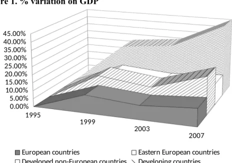
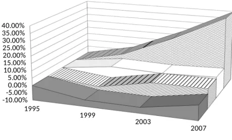
Figures 1, 2 and 3 summarize in percentage the variations of GDP, CO2 emissions and energy

consumption for the countries considered in this paper1 _{grouped in European, Eastern}

European, Developed non-European and Developed countries. The objective is to provide an overview of the main trends existing between 1995 and 2007 and to identify patterns that can be useful to explain the results obtained in the decomposition exercise. According to data reported in the following Figures, developing countries show the largest percentage variations

in GPD, CO2 emissions and energy use (+136.3%, +87.8%, +83.9% respectively between

1995 and 2007). Easter European countries also had a large variation in terms of GDP (64.7% between 1995 and 2007) and in particular after the accession to European Union in 2004 (+117% between 2004 and 2007). The energy consumption increase (+3.2%), however, have

1 _{Since data for India and Brazil are not available for the entire time period considered in the paper, these two}

been largely smaller than in the case of developing areas and the quantity of CO2 emissions

decreased (-5.3%) across the period even if a slightly increase (+2.1%) took place between 2004 and 2007 as a consequence of the economic boom [22]. In a similar way, European countries and developed non-European areas had a positive variation of GDP (+34% and 42.8%), relatively small energy consumption increase (11.9% and 12.7%) and low variations

in CO2 emissions (+5.4% and 13.4% respectively).

Figure 1. % variation on GDP

1995

1999

2003

2007 0.00%

5.00% 10.00% 15.00% 20.00% 25.00% 30.00% 35.00% 40.00% 45.00%

European countries Eastern European countries

Developed non-European countries Developing countries

Source: [9, 21]

Note: European Countries include: Austria, Belgium, Denmark, Finland, France, Germany, Greece, Ireland, Italy, Luxembourg, Netherland, Portugal, Spain, Sweden, and UK

Eastern European countries include: Czech Republic, Estonia, Hungary, Poland, Slovak Republic, and Slovenia Developed non-European countries include: Australia, Canada, Japan, South Korea, Russia, and USA

Developing countries include: China, Indonesia, Mexico, and Turkey

Figure 2. % variation on CO2 emissions

1995

1999

2003

2007 -10.00%

0.00% 10.00% 20.00% 30.00% 40.00% 50.00%

European Countries Eastern European Countries

Source: [9, 21]

Figure 3. % variations on energy consumption

1995

1999

2003

2007 -10.00%-5.00%

0.00% 5.00% 10.00% 15.00% 20.00% 25.00% 30.00% 35.00% 40.00%

European Countries Eastern European Countries

Developed Non-European Countries Developing countries

Source: [9, 21]

In general terms, a decreasing trend in the energy and in the carbon dioxide emission intensity took place across the period. According to data reported in Tables 1 and 2 all the

areas considered in this paper reduced the quantity of energy used and the quantity of CO2

emissions generated per unit of GDP. The largest percentage variations took place in the Eastern European countries that after joining the EU benefitted from energy reforms, renewable energy projects and transfer of energy and carbon efficient technologies from western European areas [23-25]. In spite of these improvements, however their carbon and the energy efficiency still remain largely lower than in the Western European countries where since the 1990s a large set of energy and carbon policies have been implemented in response to climate change concerns [26]. In terms of Developed non-European areas and Developing countries both areas performed energy and emissions intensity improvements between 1995 and 2007.

Table 1. CO2 emission intensity (CO2 emissions/GDP) (Kilotons/Millions US$)

1995 1999 2003 2007 % 2007-1995

European countries 0,37 0,34 0,32 0,29 -21,39

Eastern European countries 0,85 0,68 0,59 0,49 -42,46

Developed non-European countries 0,55 0,51 0,48 0,44 -20,53

Source: [9, 21]

Table 2. Energy intensity (Energy/GDP)(Terajoules/Millions US$)

1995 1999 2003 2007 % 2007-1995

European countries 7,04 6,69 6,53 5,88 -16,52

Eastern European countries 12,70 10,45 9,52 7,95 -37,34 Developed non-European countries 10,90 10,03 9,33 8,60 -21,06

Developing countries 11,59 9,90 9,36 9,02 -22,18

Source: [9, 21]

In the following section the data reported above are disaggregated and analysed for the 31 world countries considered in the paper.

2.2 GDP and CO2 variations:

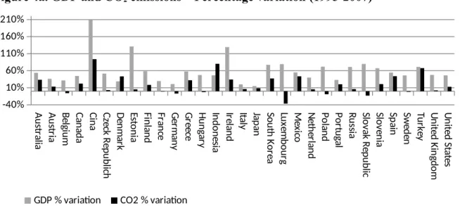
According to data reported in Figures 4a and b, all the countries considered in this paper

performed a GDP increase between 1995 and 20072_{. During the period considered, China had}

the largest percentage variations (+200.9%), followed by Estonia (+131.2%), Ireland that before the financial crash of 2008 had a GDP increase of around +129.5% and India (37.6% in just the 4 years available for this study). Poland and Slovak Republic largely benefited from joining the EU with an income variation of more than 71.9% and 79.8% respectively [22]. Luxembourg, South Korea, Russia and Turkey also performed a GDP increase higher than 70%. All the others economies, and in particular the most developed ones like United States, Canada, Belgium and France, had an income variation lower than 50%. The bottom figures are related to Germany, Denmark, Italy and Japan (+20.9%, +28.7%, + 19.9%, +14.9%, respectively). According to data reported by [27] the Italian, German and Denmark GDP have been falling since the 1990s. Between 2000 and 2012 Italy has been among the 10 world countries performing worst in terms GDP generation and Germany largely suffered for the costs of unification [28]. A vast shadow economy, limited competition and high marginal taxation rate are considered as the main factors responsible for the poor Italian performance [29, 30]. Expensive social security system and increasing level of public debt have been some of the main elements reducing GPD growth rate in the German case [31]. Deflation, reduction in capital accumulation and low level of total factor productivity growth seems to be the main

elements of Japan’s stagnation [32-34].

In terms of carbon dioxide almost all the countries considered in this paper increased the emissions between 1995 and 2007. China had the largest variation (+93.9%), even if the percentage increase has been lower than half of the percentage increase in GDP. According to data reported by [35] improvements in technologies, reduction in coal consumption and increased energy efficiency both in the industrial and in the household sectors have been the most important factors in reducing the quantity of emissions generated per unit of GDP in

China. Denmark (28.7% GDP and 43.4% CO2 emissions) and Indonesia (46.6% GDP and

80.3% CO2 emissions) are the only countries to show an increase in energy related carbon

dioxide emission higher than GDP. In the case of Indonesia a possible explanation can be related to the rapid development of manufacturing activities [36]. According to data provided by [37] the contribution of the industrial sector to the overall GDP production increased by around 5% and the consumption of coal nearly tripled during the last decade. For Denmark the main reason can be linked to the fact that the sectors that expanded the most are “water transports” and “coke, refined petroleum and nuclear fuel” characterized by a high carbon intensity rate [38]. Belgium (-5.8%), France (-1.2%), Germany (-7.1%), Hungary (-2.7%), Luxembourg (-36.4%), Poland (-9.1%), Slovak Republic (-13.1%) and Sweden (-2%) are the

only countries that reduced the quantity of CO2 between 1995 and 2007. Changes in fuels,

efficiency improvements and changes in economic activities can be the main factors responsible for this trend [39, 24, 25, 40].

Figure 4a. GDP and CO2 emissions – Percentage variation (1995-2007)

A u str ali a A u str ia B elg iu m C an ad a C in a C ze ck R ep u b lic h D en m ar k Es to n ia Fin la n d Fr an ce G er m an y G re ec e H u n ga ry In d o n es ia Ire la n d Ita

ly Jap_an Sou

th K o re a Lu xe m b o u rg M ex ico N et h er la n d P o la n d P o rtu ga l R u ss ia Slo va k R ep u b lic Slo ve n ia Sp

ain Swed

en Tu rk ey U n ite d K in gd o m U n ite d S ta te s -40% 10% 60% 110% 160% 210%

GDP % variation CO2 % variation

Figure 4b. GDP and CO2 emissions – Percentage variation (Brazil 2000-2008 and India

2004-2008)

Brazil (2000-2008) India (2004-2008)

-10% 0% 10% 20% 30% 40% 50%

GDP % variation CO2 % variation _{Source: [9, 21]}

2.3 Energy and CO2 emission intensities:

A positive aspect that contrasts with the figures of CO2 emissions increase reported by the

majority of the countries presented in Figure 1 is that in terms of energy and CO2 emission

intensities, almost all the countries considered in this paper reduced both the quantity of energy used per unit of GDP and the quantity of emissions generated per unit of energy used. According to the data reported in Figures 5a and 5b, Denmark (+10.3%), Greece (+3.9%), Indonesia (+5.9%), Turkey (+0.3%) and Brazil (+1.2% between 2000 and 2008) are the only countries that increase the energy used per unit of GDP. Denmark (+1%) and Indonesia (+16.2%), together with Canada (+4.4%), China (+0.8%), Japan (+1.6%), Netherland (+15.7%), Russia (+5.9%) and Slovenia (+1.6%) also had an increasing trend in the quantity of emission per unit of energy use. According to these data, for every unit of energy used in 2007 a larger quantity of carbon dioxide emissions are generated compared to the quantity of 1995. As reported in the previous section, possible explanations can be related to changes in technologies, to variations in the energy mix or to variations in the contribution provided by the different economic sectors to the GDP generation [24, 25, 35-40].

majority of the other European Countries [26]. China (-37.9%) and Easter European countries as Estonia (-48.7%), Poland (-42.9%), Slovak Republic (-42.6%) had the largest reduction of energy intensity. This means that the quantity of energy used to generate GDP decreased during the considered period of time. Technological improvements, together with implementation of more efficient energy strategies and adoption of EU legislations have probably been the main factors contributing to the energy improvements in the Easter European countries [24]. According to data reported by [41] the technological changes and the market based instruments promoted by the Chinese government have been key factors in reducing the energy intensity of Chinese economy. In terms of carbon dioxide, Luxembourg is the only country that improved the emission intensity by more than 50% (-62.4%). The increasing importance of low carbon intensity activities as the service and the financial sectors together with improvements on carbon efficiency and substitution between coal and natural gas, have been the main factors contributing to the emission intensity drop [42].

Figure 5a. CO2 emissions intensity and energy intensity- Percentage variation

(1995-2007) A u str ali a A u str ia B elg iu m C an ad a C in a C ze ck R ep u b lic_h D en m ar k Es to n ia Fin la n d Fr an ce G er m an y G re ec e H u n ga ry In d o n es ia Ire la n d Ita

ly Jap_an Sou

th K o re a Lu xe m b o u rg M ex ico N et h er la n d P o la n d P o rtu ga l R u ss ia Slo va k R ep u b lic Slo ve n ia Sp

ain Swed

en Tu rk ey U n ite d K in gd o m U n ite d S ta te s -70% -60% -50% -40% -30% -20% -10% 0% 10% 20%

CO2 emission intensity % variation Energy intensity % variation

Figure 5b. CO2 emissions intensity and energy intensity- Percentage variation

(2000-2008 for Brazil and 2004-(2000-2008 for India)

Brazil (2000-2008) India (2004-2008)

-14% -12% -10% -8% -6% -4% -2% 0% 2%

CO2 emission intensity % variation Energy intensity % variation

Source: [9, 21] data

To better investigate these evidences, a decomposition analysis is performed in the following section. The main objective is to identify the driving forces that contributed to the variation in the energy-related carbon dioxide emission in the 33 countries considered in this paper.

3. Decomposition analysis: methodology to identify the role of factors in the energy related CO2 emissions changes

change the energy-related CO2 emissions in different world countries. In particular, equation

[1] is used to describe CO2 emissions as a consequence of variations in energy intensity,

emission intensity and economic activity. Based on the idea that carbon dioxide emission (CE) generated by all the countries considered in this paper at time (t) can be evaluated as the product of emission intensity (CI), energy intensity (EI), economic share of a specific country

(ES) and economic activity (G) [55] express CO2 emissions as an extended Kaya identity:

CEt

=

∑

E_it × E_it GDP_it×

GDP_it

GDPt×GDP

t

=

∑

[1]

where for a specific year, Eit refers to the total energy consumption of the ith country (TJ),

GDPitrefers to the value added of the ith country, GDPtrefers to the aggregated value added

of all the considered countries and Eit refers to totalemissions (in tons) of the country i. Since

expression [1] runs from a base year 0 to a target year t, we can calculate the variation in

carbon dioxide emissions (∆CE) over the period of time ∆t as [2]:

∆CE = CEt _{– CE}0 _{= CI}

effect + EIeffect + ESeffect + Geffec [2]

where the four explanatory factors are defined as:

(i) CIeffect = CO2 intensity effect (or pollution coefficient effect). It is defined by the

ratio of CO2 emission and energy use. It reflects changes in abatement technology

and fuels quality and fuel switching. It is also named carbonisation index

(ii) EIeffect = Energy intensity effect. It refers to energy consumption per unit of output

and is defined by the ratio between energy consumption and Gross Domestic Product (GDP). It reflects changes in the structure and in the efficiency of the energy systems.

(iii) ESeffect = Structural changes effect. It is calculated as the ratio between the Gross

Domestic Product of a specific country (GDPi) and the total GDP generated by

panorama. The aim is to identify the contribution provided by every country to

the global GDP generation. Based on this equation, the ESeffect provides useful

information to identify if the underlying structure of the global economic system is changing and which countries are mainly responsible for it.

(iv) Geffect = Economic activity growth effect. It reflects changes of the total economic

activity and it is used to quantify the carbon dioxide emissions generated by economic growth.

To perform the decomposition analyses the following input data are required:

CEt _{Total CO}

2emission in year t (in tons, t);

CEt

i Total CO2emission in year t in the country i;

Et

i Total energy consumption in year t in the country i;

GDPt _{The value added in the year t;}

GDPt

i The value added in the year t in the country i;

The calculation of each component reported in equation [2], and used for decomposing the

change in CO2 emissions (∆CE) are expressed by the following equations where the sum are

intended over the individual country values and where the fractional multipliers are used according to [56] to equally distribute the residual among the decomposition factors.

Equation [3] calculates the emissions intensity effect:

[3]

CI_effect=

∑

4

∑

+1

2

∑

+1

3

∑

0

+Δ EI_i×ES_i0×ΔG+EI_i0×Δ ES_i×ΔG)

[4]

EI_effect=

∑

4

∑

+1

2

∑

+1

3

∑

0

+ΔCI_i×ES_i0×ΔG+CI_i0×Δ ES_i×ΔG)

Equation [5] calculates the structural change effect:

[5]

ES_effect=

∑

4

∑

+1

2

∑

×G0+CI_i0×Δ EI_i×Go+CI_i0×EI_i0×ΔG)+

+1

3

∑

Equation [6] calculates the economic activity growth effect:

[6]

G_effect=

∑

4

∑

+1

2

∑

×CI_i0+CI_i0×Δ EI_i×ES_i0+CI_i0×EI_i0×Δ ES_i)+

+1

3

∑

4. Results of the decomposition analysis

The decomposition results reported below, together with the data included in Tables 1 and 2 of the Appendix, are useful to identify the main reasons for carbon dioxide emission variation that took place in the 33 world countries included in the analysis. Since GDP data at constant price are not available for India and Brazil for the entire time period considered in this paper,

the results reported below includes i) a decomposition analysis for China, European Union,

Indonesia, Russia and United States for the period 1996-2008; ii) a decomposition analysis

for Brazil for the period 2000-2008 and iii) a decomposition analysis for India for the period

2004-2008.

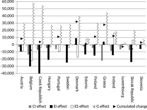
According to the results reported in Figure 6 (a, b, c and d) for all the countries considered in this paper economic growth (G effect) has been the most important driver of energy-related

the ES effect described as the relative position of a country in the total income generation, results to be an important driver for carbon dioxide emission increase particularly for China and India. The increasing role of these two fast developing economies in the international

production system is responsible for almost half of their total CO2 emission increase. In a

similar way, the increasing role on international economy played by South Korea, Russia, Turkey, Ireland and the recently eastern Europe EU Member States, like Estonia, Slovak Republic, Slovenia and Poland also contributed to increase the quantity of carbon dioxide emissions related to the relative position of these countries in the global income generation (ES effect). On the contrary, the decreasing role played in international GDP generation (ES effect) by Japan, Unites States and some of the most developed European Countries,

contributed to reduce their overall CO2 emission increase. In terms of carbon dioxide

emission intensity (CI effect) all the countries considered in this paper, exception made for Canada, China, Japan, Netherlands, Denmark, Russia, Slovenia and Indonesia, reduced the

quantity of CO2 generated per unit of energy use. The reduction in the use of natural gas and

the increasing demand for electricity, together with the increasing economic importance of sectors characterized by high carbon intensity rate, such as coke, refined petroleum, nuclear fuel activities and water transports are probably the most important factors responsible for this trend [38, 7, 57]. The reduction in the carbon dioxide intensity has been mainly generated by a set of policies oriented to reduce the carbon contents of economy. Within European Union different Directives have been devote to that. The EU Emission Trading System, the Energy Efficiency Directive, the Strategic Energy Technology Plan or the Renewable Energy Directive are just some examples. In a similar way, the Clean Air Act of United States proposed a set of policies to improve the carbon pollution standards and to promote the adoption of the best available technologies [58]. In Brazil, the large investments in hydroelectric power and the increasing use of biofuel contributed to improve the carbon intensity [59].

According to data provided by [59], the decreasing energy efficiency of Brazilian economy can be mainly explained by the fact that during the last decade economic growth has been lower than the overall energy consumption. The increasing energy demand driven by rising living standard and by the rapid growth in car ownership of the Brazilian middle class has more than double the total energy consumption. However, the low energy intensity score of Brazilian economy has large margins for improvement. The old and strained electricity network and the consequent waste in electricity transmission is one of the main factors influencing the low performance in the energy intensity reduction. The recent regulations introduced by Brazilian government in terms of standard of minimum energy performance and the large investments in the energy infrastructures are expected to improve the energy efficiency over the next decade [60, 61].

According to different studies technological changes and variation of the energy mix, particularly within the industrial sector, have been the main responsible factors for the energy intensity improvements in developing countries that usually experience a convergence trend based on their initial efficiency level [17, 62]. Transition from the industrial to the less-energy intensive sectors based on service and the rising importance of the information technologies as drivers of economic growth are considered as some of the most important factor for the developed areas [63-65, 17].

A u str ia B elg iu m C ze ck R ep u b lic h H u n ga ry P o rtu ga l Sw ed en D en m ar k Es to n ia Fin la n d G re ec e Ire la n d Lu xe m b o u rg Slo va k R ep u b lic Slo ve n ia -40,000 -30,000 -20,000 -10,000 0 10,000 20,000 30,000 40,000 50,000 60,000

CI effect EI effect ES effect G effect Cumulated change

Source: our elaboration

Figure 6b. Driving forces of CO2 emissions (Kilotons CO2 emissions)

G er m an y U

K C_an

ad a In d o n es ia M ex ico A u str ali a Sp

ain Sou

th K o re a Tu rk ey Ja p

an Italy Fran_ce

N et h er la n d P o la n d -400,000 -300,000 -200,000 -100,000 0 100,000 200,000 300,000 400,000 500,000 600,000

CI effect EI effect ES effect G effect Cumulated change

Figure 6c. Driving forces of CO2 emissions (Kilotons CO2 emissions)

C

h

in

a

U

SA Ru

ss

ia

-2,500,000 -1,500,000 -500,000 500,000 1,500,000 2,500,000 3,500,000

CI effect EI effect ES effect G effect Cumulated change

Source: our elaboration

Figure 6d. Driving forces of CO2 emissions (Kilotons CO2 emissions) (2000-2008 for

Brazil and 2004-2008 for India)

Brazil India

-250,000 -150,000 -50,000 50,000 150,000 250,000 350,000

CI effect EI effect ES effect G effect Cumulated change

The analysis presented in this paper investigates the main factors influencing the carbon dioxide emission variations that took place in 31 world countries between 1995 and 2007.

The main results show that GDP growth has been the main element responsible for CO2

emissions increase in all the countries considered in this paper. That is because the twelve years of analysis have been mainly characterized by a positive economic growth trend with some exceptional economic boom in countries as China, Estonia and Ireland. For these countries the ES effect, that summarizes the relative position of a country to the global GDP

generation, has been the largest contributors to the CO2 emission increase. To further

investigate the role played by GDP production, an interesting development of this study could be to perform a decomposition analysis for the period beyond 2007. As soon as data will be available a similar exercise will be done for the years of the financial crisis and the

subsequent economic recession. According to data provided by [66], the total CO2 emissions

from the energy sectors stalled in 2014 for the first time in 40 years. The main reasons seem to be related to the global economic downturn and to the changed patterns of energy consumption in China and OECD. Contrasting the time periods before, during and after the

recession will be very revealing of the impacts of economic trends on CO2 emissions

generation. Further to that, the analysis should be disaggregated into different economic sectors or into those groups of sectors for which the implementation of emission reductions policies are likely to produce the most effective results. Other interesting aspects of development could be related to the analysis of consumer related emissions, which considers rather than the energy used for production, the energy related to individual consumption. In this case, other decomposing factors, like income or preferences could be used to investigate the role that consumer responsibility can play in the generation of carbon dioxide emissions.

In this respect the trade links between countries and the allocation of CO2 based on consumer

activity would be relevant in identifying the non-local effects that consumer choices can

generate in the production of CO2 emissions in other world areas [49]. Additional analysis

can also be related to the application of different CO2 emissions evaluation approaches, as for

example Index or Structural Decomposition analysis and related extensions. In particular, it would be interesting to investigate how different decomposition techniques could generate

different results and how the use of different data based on different CO2 estimations

approaches can influence the overall conclusion of the analysis.

Although there exists well-known limitations in decomposition analysis [67, 68] the present

study provides a good framing of the energy-related CO2 emissions by investigating the main

factors of variations for 33 world countries. The period chosen 1995-2007 is important as it falls right within the Kyoto protocol definition and the financial crises thus setting a good

reference case for the analysis of the effects of the latter on CO2 emissions. The data used

have been taken from OECD and from the World Input-Output Database (WIOD). The main results provided in this paper show that:

 For all the countries considered economic growth (G effects) contributed to increase

the quantity of energy-related CO2 emissions.

 The increasing contribution to the global economic production provided by India

China, Russia, South Korea, Turkey, Ireland and the recently EU added eastern Europe Member States, resulted to be the second most important factor of carbon dioxide emission increase for those countries. For this group of countries, the role played by the structural change effect (ES effect) is almost comparable to the

contribution that the GDP generation provided to the overall CO2 emission increase.

On the contrary, for developed economies as Japan, United States and some of the most developed European countries, the decline in the global economic production

reduced the overall CO2 emissions increase.

 With the exceptions of Luxembourg, Finland and Ireland, the other countries that

show a positive ES factor are the rapidly growing countries. The contribution to the

global economy raises the questions on whether CO2 production should be effectively

allocated to the production country or to the countries from which the demand is generated. This question should be addressed by considering a different decomposition approach oriented to include consumption and income into the decomposition factors [69].

 In terms of carbon dioxide emission intensity (CI effect) all the countries considered

in this paper, exception made for Canada, China, Japan, Netherlands, Denmark,

Russia, Slovenia and Indonesia reduced the quantity of CO2 generated per unit of

of hydroelectric power in Brazil or the large investments in renewable energy taking place in United States and China are example of that [70].

 Denmark and Indonesia, together with Greece, Turkey and Brazil are also the only

countries for which the energy intensity (EI effect) of the overall economic system increased during the considered period. This means that for every unit of GDP production a larger quantity of energy was needed in 2007 compared to quantity used in 1995. Policies for energy efficiency, adoption of best available technologies and consumers responsibilities have been some of the main factors contributing to reduce the energy intensity of developed and developing countries [71].

In our view the current study sets a good benchmarking case for the assessment of energy related CO2 emissions. It will be interesting to contrast these results to the post Kyoto period 2005-2020 and especially to the effects of the crises not only on the emission but also on how an externally driven G factor can modify the emission trend and whether technological improvements have taken place in such a low economy regime.

Disclaimer

The views expressed are purely those of the authors and may not in any circumstances be regarded as stating an official position of the European Commission.

References

[1] NOAA - National Oceanic & Atmospheric Administration, U.S. Department of

Commerce e NOAA. Trends in atmospheric carbon dioxide. 2009 Available at:

www.esrl.noaa.gov/gmd/ccgg/trends/

[2] Lüthi D, Le Floch M, Bereiter B, Blunier T, Barnola JM, Siegenthaler U, et al. High-resolution carbon dioxide concentration record 650,000-800,000 years before present. Nature 2008;453:379-82.

[3] IPCC. Greenhouse gas inventory: IPCC guidelines for national greenhouse gas inventories. Bracknell, England: United Kingdom Meteorological Office. 1995

[5] OECD. Indicators to measure decoupling of environmental pressure from economic growth. Paris: OECD. 2002. Available at: http://www.olis.oecd.org/olis/ 2002doc.nsf/LinkTo/sg-sd

[6] IEA – International Environmetnal Agency, 2015. Available at:

http://www.iea.org/newsroomandevents/news/2015/march/global-energy-related-emissions-of-carbon-dioxide-stalled-in-2014.html

[7] Voigt S, De Cian E, Schymura M, Verdolini E. 2014. Energy intensity development in 40 major economies: structural changes or technological improvement? Energy Economics 2004;41:47-62

[8] Allcott H, Greenstone M. Is There an Energy Efficiency Gap?. Journal of Economic Perspectives 2012;26(1):3-28.

[9] World Input-Output Database (WIOD) : www.wiod.org

[10] Sue Wing I. Explaining the declining energy intensity of the U.S Resour. Energy Econ. 2008;30:21–49

[11] Huntington H.G. Structural change and U.S. energy use: recent patterns Energy 2000;31: 25–39

[12] Fisher-Vanden K, Jefferson GH, Liu H, Tao Q. What is driving China's decline in energy intensity? Resour. Energy Econ. 2004;26,77–97

[13] Ma C, Stern DI. China's changing energy intensity trend: a decomposition analysis Energy Econ. 2008;30(3):1037–1053

[14] Wu Y. Energy intensity and its determinants in China's regional economies, Energy Policy 2012;41: 703–711

[15] Zhang Z, Why did the energy intensity fall in China's industry sector in the 1990s? The relative importance of structural change and intensity change Energy Econ. 2003;25:625–638

[16] Sanstad AH, Roy J, Sathaye JA. Estimating energy-augmenting technological change in developing country industries Energy Econ. 006;28: 720–729

[17] Mulder, P, De Groot HLF. Structural change and convergence of energy intensity across OECD countries, 1970–2005. Energy Econ. 2012;34(6):1910–1921

[18] Greening LA, Davis WB, Schipper L. Decomposition of aggregate carbon intensity for the manufacturing sector: comparison of declining trends from 10 OECD countries for the period 1971–1991 Energy Econ. 1998;20:43–65

[20] Dietzenbacher E, Los B. Stehrer R, Timmer M, Gaaitzen de V. The Construction of World Input-Output Tables in the Wiod Project. Economic Systems Research 2013;25:71-89

[21] OECD Database: http://stats.oecd.org/

[22] EBRD – European Bank of Reconstruction and Development, 2013. Transition Report 2013. Stuck in Transition. EBRD, London, 2013

[23] Regional Environmental Center: www.rec.org

[24] ECF – European Climate Foundation. Roadmap 2050. A practical guide to a prosperous,

low-carbon Europe. 2011 Available at: www.roadmap2050.eu

[25] Budzianowski WM. Target for national carbon intensity of energy by 2050: A case study of Poland’s energy system. Energy 2012;46:575-581

[26] Henriques ST, Borowiecki KJ. The drivers of long-run CO2 emissions: a global

perspective since 1800. Trinity Economic Papers – Working Paper No. 0314, September 2014

[27] Balcerowicz L, Rzonca A, Kalina L, Laszek A. Economic growth in the European Union. Lisbon Council E-Book, Brussels, 2013

[28] IMF – International Monetary Fund. Germany: Staff Report for the Article IV Consultations with Germany. Washington: IMF, 2011

[29] Lusinyan L, Muir D. Assessing the Macroeconomic Impact of Structural Reforms. The Case of Italy. IMF Working Papers 13/22, 2013

[30] IMF – International Monetary Fund. Italy: Staff Report for the 2011 Article IV Consultation with Italy. IMF Country Report No. 11/173, 2011

[31] Graf B, Rakau O, Schneider S. Focus on Germany, Current Issues. London: Deutsche Bank Markets Research, 2013

[32] Koo RC. Balance Sheet Recession: Japan’s Struggle with Uncharted Economics and its Global Implications. Singapore: John Wiley & Sons (Asia) Pte Ltd, 2003

[33] Hamada K, Horiuchi A. Wrap-up Comments: Prolonged Stagnation Occurred. In: Hamada K, Horiuchi A, and ESRI, Cabinet Office, Eds., Discussions on Japan’s Economic Crisis: An Investigation into True Causes of Japan’s Prolonged Stagnation, Nikkei, pp. 289-340, 2004

[34] Caballero RJ, Tokeo JH, Kashyap AK. Zombie Lending and Depressed Restructuring in Japan. American Economic Review 2008;98(5):1943-1977

[35] Feng K, Hubacek K, Guan D. Lifestyles, technology and CO2 emissions in China: A

[36] Imansyah MH, Putranti TM, Affandi DY, Khafian N, Tambunan M. The Key Sectors in

CO2 emission in Indonesia: Input-Output Analysis. International Journal of

Administrative Science & Organization 2013;20(1):45-50 [37] World Bank Database: data.worldbank.org

[38] Gazheli A, Antal M, van den Bergh J.. Sector-level tests of the feasibility of green growth: Carbon intensity versus economic and productivity growth indicators. Working Paper No.81, 2015 - WWWFOREUROPE Project. Available at:

http://www.foreurope.eu/fileadmin/documents/pdf/Workingpapers/WWWforEurope_WP S_no081_MS212.pdf

[39] SEI – Stockholm Environmental Institute. Evaluating Sweden’s emissions: at home and

abroad. 2008 Available at:

http://www.sei-international.org/mediamanager/documents/Publications/Rethinking-development/Global_assessments/Evaluating-Swedens-emissions.pdf

[40] Petrick S. Carbon Efficiency, Technology, and the Role of Innovation Patterns: Evidence from German Plant-Level Microdata. Kiel Working Paper No. 1833, 2013

[41] World Bank:

http://www.worldbank.org/en/news/feature/2014/06/27/bringing-chinas-energy-efficiency-experience-to-the-world-knowledge-exchange-with-asian-countries

[42] Enerdata, 2011. Luxembourg: Energy Efficiency Report. Available at:

http://www05.abb.com/global/scot/scot316.nsf/veritydisplay/3abc548fff4d870ac12578dc 002db3e9/$file/luxembourg.pdf

[43] Hoekstra R, van den Bergh JCJM. Comparing structural decomposition analysis and index. Energy Economics 2003;25(1):39-64

[44] Feng K, Hubacek K, Guan D. Lifestyles, technology and CO2 emissions in China: A

regional comparative analysis. Ecological Economics 2009;69:145-154

[45] Ang BW, Zhang FP. A survey of index decomposition analysis in energy and environmental studies. Energy 2000;25(12):1149-76.

[46] Su B, Ang B.W. Structural decomposition analysis applied to energy and emissions: Some methodological development. Energy Economics 2012;34(1):177-188

[47] Wachsmann U, Wood R, Lenzen M, Schaefer R. Structural decomposition of energy use in Brazil from 1970 to 1996. Applied Energy 2009;86(4):578-587.

[48] Ang BW, Xu XY, Su B. Multi-country comparisons of energy performance: The index

decomposition analysis approach. Energy Economics 2015;47:68-76

[49] Xu Y, Dietzenbacher E. A structural decomposition analysis of the emissions embodied

[50] Xu XY, Ang BW. Analysing residential energy consumption using index decomposition analysis. Applied Energy 2013;113:342-251

[51] Andreoni V, Galmarini S. Decoupling economic growth from carbon dioxide emission: a decomposition analysis of Italian energy consumption. Energy 2012;44:682-691

[52] Andreoni V, Galmarini S. European CO2 emission trend: A decomposition analysis for

water and aviation transport sector. Energy 2012;45:595-602

[53] Cellura M., Longo S, Mistretta M. Application of the Structural Decomposition Analysis to assess the indirect energy consumption and air emission changes related to Italian households consumption. Renewable and Sustainable Energy Reviews 2012;6(2):1135-1145

[54] Hammond GP, Norman JB. Decomposition analysis of energy-related carbon emissions from UK manufacturing. Energy 2012;41(1):220-227

[55] Sun JW. Accounting for energy use in China, 1980-94. Energy 1998;23:835-849.

[56] Shyamal P, Bhattacharya RN. CO2 emission from energy use in India: a decomposition analysis. Energy Policy 2004;32:585-593.

[57] Natural Resource Canada. Summary Report on Energy Use in the Canadian Manufacturing Sector 1995-2008. Energy Publication - Natural Resource Canada, Ottawa, 2010

[58] EPA Website: http://www.epa.gov/air/caa

[59] Luomi M. Sustainable Energy in Brazil: Reversing Past Achievement or Realizing Future Potential. The Oxford Intsitute for Energy Study 2014; pp.55

[60] Nogueira HLA., Cardoso RB., Cavalcanti CZB., Leonelli PA. Evaluation of the energy impacts of the Energy Efficiency Law in Brazil. Energy for Sustainable Development 2015;24:58-69

[61] IPEEC. Energy Efficiency Report Brazil. 2012 Available at:

file:///C:/Users/andreov/Downloads/1397575956Brazil%20Country%20report %20(FINAL%20and%20UPDATED%20April%202014).pdf

[62] Jakob M, Haller M, Marschinski R. Will history repeat itself? Economic convergence and convergence in energy use patterns. Energy Economics 2012;34:95–104

[63] Parcebois, J. Economie de l’energie. Paris: Economica, 1989

[64] Heriques ST, Kander A. The modest environmental relief from a transition to the service economy. Ecological Economics 2010;70(2):271-282

Kingdom and the US during 100 years of economic growth. Ecological Economics 2010;69:1904-1917

[66] IEA – International Environmental Agency, 2015. Available at:

http://www.iea.org/newsroomandevents/news/2015/march/global-energy-related-emissions-of-carbon-dioxide-stalled-in-2014.html

[67] Ang BW, Liu N. Viewpoint: Energy decomposition analysis: IEA model versus other

methods, Energy policy 2007;35:1426‐1432.

[68] Janssens-Maenhout G, Paruolo P, Martelli S. Analysis of Greenhouse Gas Emission Trends and Drivers, JRC SCIENCE and Policy report, JRC 78707, EUR 25814 EN, doi: 10.2788/84075, pp 45, 2013

[69] Arto, I, Rueda-Cantuche, JM, Andreoni, V, Mongelli, I, Genty, A. The game of trading jobs for emissions, Energy Policy 2014;66:517-525

[70] UNEP, 2015. Global Trends in Renewable Energy Investment. Available at: http://fs-unep-centre.org/publications/global-trends-renewable-energy-investment-2015

[71] Expert Group on Energy Efficiency. Revitalizing the Potential for Energy Efficiency –

Appendix 1. Decomposition of CO2 emissions (Kilotones)

Country

Time period

CI effect EI effect ES effect G effect Cumulated change

2007-2003 -3,632.9 -116,083.7 -81,962.4 160,887.7 -40,791.3 2007-1995 -71,773.9 -175,418.9 -238,283.9 418,583.4 -66,893.4 Greece 1999-1995 -2,758.4 2,357.3 -1,213.2 12,783.3 11,169.0 2003-1999 -9,364.5 2,546.7 4,971.1 13,283.0 11,436.4 2007-2003 -10,829.2 -1,241.3 -2,645.2 19,850.9 5,135.3 2007-1995 -22,189.8 3,978.4 1,146.7 44,805.4 27,740.7 Hungary 1999-1995 -4,647.2 -3,173.9 -2,114.8 8,371.1 -1,564.8 2003-1999 2,250.4 -10,110.0 1,888.9 7,760.9 1,790.3 2007-2003 -2,304.2 -7,145.2 -3,154.4 10,713.0 -1,890.8 2007-1995 -4,813.9 -20,839.9 -3,458.3 27,446.7 -1,665.3 Indonesia 1999-1995 18,494.0 49,489.2 -37,387.2 34,279.4 64,875.4 2003-1999 10,019.1 -1,339.0 14,294.4 39,783.0 62,757.5 2007-2003 15,774.3 -51,140.1 15,457.2 64,754.2 44,845.7 2007-1995 44,457.3 16,930.4 -18,595.7 129,686.5 172,478.5 Ireland 1999-1995 -1,989.3 -6,176.4 9,702.4 5,397.0 6,933.8 2003-1999 -2,530.8 -5,169.3 4,835.0 5,605.6 2,740.5 2007-2003 -4,182.2 -2,760.5 1,156.3 8,192.4 2,405.9 2007-1995 -8,552.9 -14,469.2 16,323.5 18,778.8 12,080.1 Italy 1999-1995 -16,000.6 4,899.3 -37,239.8 64,336.6 15,995.6 2003-1999 -6,345.7 4,822.1 -33,951.5 62,184.7 26,709.5 2007-2003 -32,390.2 -13,516.0 -55,289.0 87,260.1 -13,935.1 2007-1995 -54,449.3 -3,329.4 -126,202.9 212,751.6 28,770.0 Japan 1999-1995 421.0 21,430.7 -139,501.7 161,968.1 44,318.0 2003-1999 62,717.2 -71,002.6 -100,554.5 155,564.8 46,724.8 2007-2003 -44,889.3 -40,667.6 -127,161.5 219,853.0 7,134.7 2007-1995 19,433.6 -89,053.1 -372,645.7 540,442.6 98,177.5 South Korea 1999-1995 -32,152.0 -7,672.6 12,617.6 59,083.5 31,876.4 2003-1999 -23,098.4 -17,339.6 43,266.3 60,674.4 63,502.7 2007-2003 -8,001.0 -32,811.8 3,734.0 94,544.7 57,465.9 2007-1995 -68,678.1 -57,193.8 62,777.1 215,939.9 152,845.1 Luxembour

g 1999-1995 -2,432.7 -452.7 556.6 998.0 -1,330.8

2003-1999 -2,836.0 389.9 197.1 744.3 -1,504.7

2007-2003 -695.1 -319.7 142.3 879.2 6.7

2007-1995 -28,105.6 -204,239.4 35,528.2 163,443.5 -33,373.4 Portugal 1999-1995 -113.3 2,147.2 1,831.4 8,334.2 12,199.5 2003-1999 -3,521.8 -290.8 -4,784.5 8,533.6 -63.5 2007-2003 -2,943.9 -2,177.1 -7,673.3 11,700.1 -1,094.2 2007-1995 -6,043.8 -99.8 -9,595.6 26,780.9 11,041.8 Russia 1999-1995 31,969.8 -97,284.0 -243,414.8 218,045.8 -90,683.1 2003-1999 35,796.7 -336,004.6 211,730.3 203,386.4 114,908.9 2007-2003 24,453.0 -440,625.4 192,264.1 298,530.1 74,621.9 2007-1995 99,241.9 -926,104.6 159,771.4 765,938.9 98,847.7 Slovak

Republic 1999-1995 -2,376.9 -6,787.3 642.2 6,063.6 -2,458.3 2003-1999 -4,054.7 -1,997.8 457.8 5,426.8 -168.0 2007-2003 -870.3 -14,408.5 4,779.4 7,277.8 -3,221.6 2007-1995 -7,484.5 -24,086.0 6,212.3 19,510.2 -5,847.9

Slovenia 1999-1995 -715.7 -1,774.2 478.4 2,094.0 82.5

2003-1999 388.3 -1,082.8 138.3 2,030.6 1,474.4

2007-2003 668.1 -2,691.3 508.7 3,080.2 1,565.7

2007-1995 262.1 -5,800.4 1,180.0 7,480.8 3,122.6

Spain 1999-1995 -80.0 -418.7 3,652.6 38,035.2 41,189.1

2003-1999 -17,138.3 9,172.5 4,390.9 40,208.7 36,633.9 2007-2003 -3,253.9 -12,245.1 -12,514.1 61,812.0 33,798.9 2007-1995 -20,044.1 -2,276.8 -2,646.1 136,588.8 111,621.9 Sweden 1999-1995 -3,530.2 -6,143.0 -593.8 8,724.8 -1,542.2 2003-1999 5,267.2 -9,763.2 -1,560.3 8,105.0 2,048.6 2007-2003 -2,787.4 -8,312.8 -1,897.6 11,222.4 -1,775.3 2007-1995 -1,086.8 -24,782.4 -4,145.3 28,745.6 -1,268.9 Turkey 1999-1995 -4,349.6 1,737.4 -457.3 26,483.5 23,414.1 2003-1999 -1,793.4 5,955.5 -2,266.9 27,884.0 29,779.2 2007-2003 2,089.1 -8,876.3 27,908.4 46,951.9 68,073.1 2007-1995 -5,532.7 749.2 21,956.0 104,093.8 121,266.4 United

Kingdom 1999-1995 -39,702.9 -42,296.8 1,184.7 82,212.1 1,397.1 2003-1999 21,438.8 -72,744.1 -1,636.3 77,675.3 24,733.8 2007-2003 10,929.9 -99,174.2 -32,667.4 108,660.3 -12,251.4 2007-1995 -8,465.3 -216,845.6 -33,117.6 272,307.9 13,879.4 United

Appendix 2. Decomposition of CO2 emissions (Kilotones) – Brazil and India

Country

Time period CI effect EI effect ES effect G effect Cumulated change

Brazil 2008-2000 -36,349.0 3,904.4 -22,579.4 113,787.5 58,763.5