R E S E A R C H
Open Access
Extensivity in infinitely large multiplex
networks
Maria Angélica Araujo
*and Murilo S. Baptista
*Correspondence: [email protected] Institute of Complex Sciences and Mathematical Biology, University of Aberdeen, SUPA, AB24 3UE Aberdeen, UK
Abstract
In this paper, we investigate the relationship between the coupling strengths and the extensive behaviour of the sum of the positive Lyapunov exponents of multiplex networks formed by coupled dynamical units. Considering networks where the dynamics of the nodes is given by the shift map, we do not only demonstrate which are the relevant parameters leading to extensivity, but also provide exact formulas how they are related. A distinct result was to show that it is always possible to construct infinitely large extensive networks by attaching, with rescaled inter-connections, infinitely many smaller networks. These smaller networks are effectively the building blocks of the large network. This is because these building blocks can have arbitrary topology and the strength of connections among nodes only depends on the block size, and not on the size of the whole network.
Keywords: Extensivity, Multiplex networks, Lyapunov exponents
Introduction
Complex networks are structures consisting of nodes and edges, which are connected in a non-trivial way (Boccaletti et al.2006; E J Newman2010; Strogatz2001; Estrada2015). The theory of complex networks has been studied across many fields, such as sociology, biology, mathematics, physics and computer science and a wide variety of phenomena are described by complex networks, from a microscopic level as in complex brain networks (Bullmore and Sporns2009) to macroscopic systems of social interactions (Robins et al.
2007) and technological systems (Nardelli et al.2014), for instance.
An important concept that can play a significant role in the understanding of complex dynamical networks is extensivity. A quantity is extensive, if it scales directly with the size of the system. Extensive quantities are additive for subsystems, which means that, physical systems that are extensive can be decomposed into independent subsystems that could also be extensive. The reverse is also true. Extensive systems can be constructed by putting together independent subsystems, for example, adding more mass to a body.
The concept of extensive quantities can be extended to the scope of complex systems. Ruelle was the first to infer the extensivity of chaos (Ruelle 1982). The most common and practical procedure to identify chaos in complex systems is computing the Lyapunov Exponents (LEs), which measure the rate of separation of infinitesimal close trajectories in phase space (Eckmann and Ruelle1985; Ott2002). Then, according to Ruelle, extensiv-ity can be understood by studying the curve of LEs, when arranged in descending order,
as function of the their normalised index and calculated at different system sizes. If these curves collapse onto a single asymptotic spectrum as the system size grows, then chaos is considered to be extensive. A direct consequence of this is that, the sum of the positive LEs is linearly related to the size of the network. Moreover, extensive systems can be typi-cally decomposed into smaller fundamental units that could imply that a large dynamical network with complex topology could be broken down into “independent” subnetworks with similar dynamic properties.
Extensive chaos has been discussed in many complex systems. In globally coupled dynamical systems, although all the elements of the system are subject to the same influ-ences, the nontrivial connection between their components can give rise to collective chaos (Shibata and Kaneko 1998) and nonextensive behaviour (Takeuchi et al. 2011). Due to the nontrivial collective behaviour in these type of systems, the extensivity of the Lyapunov exponents has been contested in (Takeuchi et al. 2009). In contrast to this, extensivity has been commonly observed, for instance, by studying the spatiotem-poral chaos, in Rayleigh-Bénard convection (Paul et al.2007) and in reaction-diffusion networks (Stahlke and Wackerbauer2009; 2011).
For high-dimension systems, we can mention the results in (Karimi and Paul 2010), where the authors investigated the extensive chaos behaviour of the Lorenz-96 model by studying the variation of the fractal dimension for different parameters of the sys-tem. In (Xi et al.2000), Xi et al. studied the extensivity of the Lyapunov dimension and the Kolmogorov-Sinai entropy in the one-dimensional Nikolaevskii model. Extensivity of chaos was also detected in large sparse neuron networks (Monteforte and Wolf2010) and in different classes of sparse random networks (Luccioli et al.2012). In the latter, the authors have explored the relationship between the number of incoming connections per node and the extensive behaviour, when all nodes are subject to the same connectivity.
In this paper, we study analytically how extensivity of the sum of the positive Lyapunov exponents of networks of coupled shift maps, but where the topology of the couplings fol-lows a “multiplex” topology, can be maintained by smartly changing the configuration of the network as it grows in size. So, the topology of the constructed network of interacting units is a network of many subnetworks. A subnetwork is a set of dynamical units coupled by an intra topology and an intra coupling strength. Subnetworks are connected by the so called inter topology with inter coupling strength. A main point of interest in this work is to understand the role of the intra and inter-couplings in the extensive behaviour of large multiplex networks. Our extensive quantity, the sum of the positive Lyapunov exponents, denoted byHKS, is an upper bound for the Kolmogorov-Sinai entropy. In contrast to the
entropy,HKScan be usually well estimated, even in networks with arbitrary sizes.
Moreover, we also show that, given an initial dynamical network with an arbitrary intra-connectivity topology, it is always possible to construct an infinitely large extensive network with an infinite number of these initial networks, the building blocks, connected with rescaled inter-link strengths. This result reinforces the idea that an extensive com-plex network can be broken down into building blocks that are also extensive. Since all our calculations are exact, we provide a reliable and practical method to achieve extensivity.
Methods
Consider, initially, a network(0)withN
0nodes where the dynamics of the nodes is given
by the shift mapFx(ni)
=2x(ni)(mod 1), i.e.:
x(ni+)1=2x(ni)−ε
N0
j=1
Aijx(nj) (mod 1), (1)
whereεrepresents the coupling strength of the intra-connections andA=(Aij)denotes
the Laplacian matrix. The main motivation to use this map is the fact that it is a trans-formation with constant Jacobian, allowing for an analytical calculation of the LEs for networks constructed with this map. Moreover, this paper extends previous results in the works (Antonopoulos and Baptista2017) and (Baptista et al.2016). The (mod 1) is a modular function that guarantees that the transformed point (by 2x) remains in the interval [ 0, 1].
Now, let(1)be the network constructed by coupling two equal subnetworks(0), then its number of nodes isN1=2N0and it can be represented by:
x(ni+)1=2x(ni)−ε
N1
j=1
Gijx(nj)−γ α N1
j=1
Lijx(nj) (mod 1), (2)
whereγ is the coupling strength of the inter-connections,α= l12
N0 is the ratio between the number of inter-connectionsl12andN0. The Laplacian matrices of the intra and
inter-connections are represented byG=(Gij)andL=(Lij), respectively. Therefore, they are
given by:
G=
A 0 0 A
and L=
D1 −B
−BT D2
, (3)
where0denotes theN0×N0zero matrix,T stands for the transpose andBrepresents
the adjacency matrix of the inter-connections. The matricesD1andD2are the diagonal
degree matrices of the adjacency matricesBandBT, respectively. Their components are defined as:
(D1)ii= N0
j=1
Bij and (D2)ii= N0
j=1
BTij, for i=1,. . .,N0. (4)
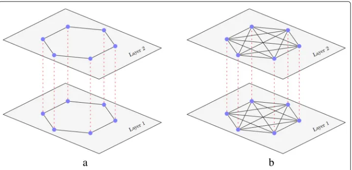
We suppose that the intra and inter-connections are undirected, i.e., each connection between the nodes is bidirectional. Besides, we consider a diagonal interlinking configura-tion, which means that each node in a subnetwork is only connected to the corresponding node in the other equal subnetwork, consequentlyl12 = N0andα = 1. Figure1
illus-trates this configuration in networks where the building blocks haveN0= 6 nodes with
Fig. 1Examples of the diagonal interlink configuration. Each network is formed by two equal subnetworks withN0=6 nodes each and, with (a) ring and (b) all-to-all topology. The solid black and dashed red links
correspond to the intra and inter-connections, respectively
We can rewrite Eq. (2) in a matrix form as:
xn+1=2xn−M1xn (mod 1), (5)
whereM1=
εA+γ αD1 −γ αB
−γ αBT εA+γ αD2
. DefiningJ1=2I1−M1, whereI1represents
theN1×N1identity matrix, Eq. (5) becomes:
xn+1=J1xn (mod 1). (6)
Since all the connections are undirected, the matrix M1 is symmetric as well as the
Jacobian matrixJ1. The Lyapunov exponent of Eq. (6) in the direction of a vectorv∈RN1
is given by, (Ott2002):
λ(v)= lim
N−→∞
1 N ln J
N
1 ·v , (7)
where · represents the Euclidean norm inRN1.
Letλ(i1), fori=0,. . .,N1−1, be the unordered (and possibly not all distinct) Lyapunov
exponents of Eq. (6). As consequence of the JacobianJ1being constant and symmetric we have that:
λ(1)
i =lnθ(
1)
i , fori=0,. . .,N1−1, (8)
where θi(1) represents the eigenvalues of the matrix J1 and | · | denotes the absolute value. This result is demonstrated in (Araujo and Baptista: A comprehensive review about Lyapunov Exponents in continuous and discrete dynamical networks, in preparation). Note that, if we denote byμ(i1)the eigenvalues ofM1fori=0,. . .,N1−1, then:
θ(1)
i =2−μ(
1)
i . (9)
Thus, Eq. (8) can be written as:
λ(1)
i =ln2−μ(
1)
i . (10)
By (Baptista et al.2016; Martín-Hernández et al.2014), the unordered eigenvalues of
μ(1)
2i = εωi (11)
μ(1)
2i+1 = εωi+2γ α, (12)
fori = 0,. . .,N0−1 and where 0 = ω0 ω1 . . . ωN0−1represent the ordered eigenvalues of the Laplacian matrixA. Note that,μ(21i)are the eigenvalues coming from one layer, whereasμ(21i+)1are the eigenvalues due to the inter-connectivity, generated by perturbingμ(21i)with the term 2γ α.
The main goal of this work is to grow the network(1) and to study the conditions
to have the sum of the positive LEs of each network linearly proportional to its number of nodes. This growing is made as following:(2) is constructed by coupling two equal subnetworks(1)with the same parameterαand with the same diagonal interlinking con-figuration. The number of nodes of(2)isN2=2N1=22N0and it can be represented by:
xn+1=2xn−M2xn≡J2xn (mod 1), (13)
where the matricesM2andJ2are constructed in the same way asM1andJ1, respectively. The eigenvalues ofM2are given by:
μ(2)
4i = εωi (14)
μ(2)
4i+1 = εωi+2γ α (15)
μ(2)
4i+2 = εωi+2γ α (16)
μ(2)
4i+3 = εωi+4γ α, (17)
fori=0,. . .,N0−1. Similar to how the eigenvalues ofM1were generated, the setμ(2)≡
μ(2) 4i ,μ
(2) 4i+1
are the eigenvalues due to the layer(1)and
μ(2)
4i+2,μ
(2) 4i+3
are generated by perturbing the setμ(2)with 2γ α.
Proceeding this way, the network(k) with a number of nodes given byNk = 2kN0
is constructed by coupling two equal subnetworks(k−1)with the same parameters and configuration. Thus, as a result of this recursive procedure for generating self-similar net-works each layer is connected to all the other layers in the network, and Fig.1represents only the first step of this process. The inter-coupling strength,γ, will be rescaled in order to maintain the extensive property of the network as it grows. The distinct eigenvalues of the corresponding matrixMkfor the network(k)are:
˜
μ(k)
0,i ≡ εωi (18)
˜
μ(k)
1,i ≡ εωi+2γ α (19)
˜
μ(k)
2,i ≡ εωi+4γ α (20)
.. .
˜
μ(k)
j,i ≡εωi+2jγ α
.. .
(21)
˜
μ(k)
j=(k−1),i≡εωi+2(k−1)γ α (22)
˜
μ(k)
Note that, the set of eigenvaluesμ˜(j,ki)repeatskj= j!(kk−!j)! times, forj=0,. . .,k. Also note that, for a fixedj, the eigenvalues in the setμ˜(j,ki)are all distinct iff all theωiare, for
i=0,. . .,N0−1.
In the next section, we explore analytically the conditions for the network(k)to have extensive behaviour. Here, extensivity implies that the sum of the positive LEs,HKS =
λ(k)
i >0λ
(k)
i , is a linear function of the size of the system,Nk.
Results
As we have seen, the LEs of(k)are computed by: λ(k)
i =ln2−μ( k)
i , (24)
whereμ(ik)are the eigenvalues ofMk, fori=0,. . .,Nk−1. The LEs of(k)can be divided
into two sets, ε(computed fromμ˜(0,ki), fori=0,. . .,N0−1), that represents the LEs that
only depend on the intra-coupling strength, and γ,ε (computed from the eigenvalues ˜
μ(k)
j,i , forj=1,. . .,kandi=0,. . .,N0−1), formed by the ones that depend on both, the
intra and inter-coupling strengths (Baptista et al.2016; Martín-Hernández et al. 2014). We have explored analytically the conditions for the network(k)to have the sum of the positive LEs extensive in three different situations.
Case 1
In our first analysis we consider networks having only positive LEs, which leads to maxi-mal values ofHKS. Then, assuming that all elements of εand γ,εare positive we have that:
ln|2−εωi| > 0 and, (25)
ln|2−εωi−2jγ α| > 0, (26)
for everyi=0,. . .,N0−1 andj=1,. . .k. Therefore:
HKS = Nk−1
i=0
λi= Nk−1
i=0
ln2−μ(ik)=
k
j=0
N0−1
i=0
k j
ln2− ˜μ(j,ki) (27)
=
k
j=0
N0−1
i=0
k j
ln2−εωi−2jγ α (28)
=
k
j=0
N0−1
i=0
k j
ln2
1− εωi 2 −jγ α
(29)
=
k
j=0
N0−1
i=0
k
j ln(2)+ln
1−εωi
2 −jγ α
(30)
=
k
j=0
k j
N0−1
i=0
ln(2)+
k
j=0
N0−1
i=0
k j
ln1−εωi 2 −jγ α
= 2kN0ln(2)+
k
j=0
N0−1
i=0
k j
ln1− εωi 2 −jγ α
(32)
= Nkln(2)+
k
j=0
N0−1
i=0
k j
ln1−εωi 2 −jγ α
. (33)
Equation (33) does not allow to determine explicitly the dependence ofHKSonNk. To
this analysis we will expand the logarithm function. In order to consider the Maclaurin expansion up to first order of ln1−εωi
2 −jγ αin Eq. (33), assume that:
εωi
2 +jγ α
1, (34)
for everyi=0,. . .,N0−1 andj=0,. . .,k. Consequently, for eachiandjwe have that:
0<1− εωi
2 −jγ α2, (35)
and then, we can omit the absolute value in Eq. (33). Rewriting it we have:
HKS Nkln(2)+ k
j=0
N0−1
i=0
k j −
εωi
2 −jγ α
(36)
= Nkln(2)− k
j=0
k j
N0−1
i=0
εωi
2 −
N0−1
i=0
k
j=0
k j
jγ α (37)
= Nkln(2)−2k−1ε N0−1
i=0
ωi−N0γ α
k
j=0
k j
j (38)
= Nkln(2)−2k−1ε N0−1
i=0
ωi−N0γ α
k2k−1
(39)
=Nkln(2)−2k−1εS−2k−1N0αγk (40)
=Nkln(2)−
Nk
2N0ε
S−Nk
2 αγk (41)
=Nk
ln(2)− εS 2N0
−Nk
2 αγk (42)
=aNk+b(k), (43)
where:
S=
N0−1
i=0
ωi, a=ln(2)− ε
S 2N0
and b(k)= −Nk
2 αγk. (44)
It is now clear the dependence ofHKSonNk. Let us discuss some of the main features
of this. Note that, once we have set the building block with an intra-coupling strengthε, the numberain Eq. (43) is a constant and does not depend onk. However, the same is not true for the termb(k), that as we can see, depend strongly on the numberk. Our goal is to haveHKSas a linear function ofNk, which implies in havingb(k)as a constant or
only proportional toNk. Therefore, in order to satisfy the latter, i.e.,b(k)=dNk, whered
b(k)= −αcNk
2 and HKSaNk, (45)
wherea =a−α2c.
On the other hand, in order to satisfy conditions (25) and (26) without contradicting inequality (34) we must have:
εωi<1 and εωi+2jαγ <1, (46)
for eachi=0,. . .,N0−1 andj=1,. . .,k. Note that, 0ωiN0for eachi=0,. . .,N0−
1 and remember we are considering thatα = 1. Then, aiming to satisfy conditions (34) and (46) simultaneously we need to choose the parametersεandγ such that:
ε 1 N0
and, (47)
γ 1−εN0
2k . (48)
Combining condition (48) with the fact thatγ should be taken inversely proportional tok, we have that:
γ≡γ (k)= 1−εN0
2kC , (49)
for a constantC, such thatC 1. Therefore, if conditions (47) and (49) are satisfied we maintain extensivity keeping all LEs positive as the network grows.
For the networks considered and that have a great deal of symmetry, connectivity and size must be interlinked to create extensivity. In single networks, fully connected, the rescaling to create extensivity would requireεto be much less thanN1
0. To networks con-sidered in here, our results show that, the intra-coupling must be bounded by the inverse of the number of nodes of the building block, which can be set as a constant, before the growing process starts. It is the inter-coupling that must be rescaled, and the rescaling depends on the number of times (given byk) that the network has evolved.
Case 2
In the second case, we assume that(k) has positive as well as negative LEs and that the inter-coupling strengthγ is responsible for the change in the sign of the LEs, i.e., all elements of εare positive and we do not have any restrictions for the ones that comes from γ,ε. Then:
ln|2−εωi|>0, (50)
for everyi = 0,. . .,N0−1. Letnbe the number of negative LEs and define bypthe
number of positive ones. For eachi∈ {0,. . .,N0−1}andj∈ {1,. . .,k}define:
λij=ln2−εωi−2jγ α. (51)
Then, consider the setAdefined by:
A= {λiljl |il=i,jl=jandλij>0}, (52)
i.e.,Ais formed by the elementsλijthat are positive. Letqbe its cardinality. The setA
may contain repeated elements, for instance, if the LEλij appears “×" times, thenλij
Therefore, the sum of the positive LEs is given by:
HKS= N0−1
i=0
ln|2−εωi| + q
l=1
k jl
λiljl (53)
=
N0−1
i=0
ln|2−εωi| + q
l=1
k jl
ln2−εωil −2jlαγ (54)
=
N0−1
i=0
ln21−εωi 2
+q
l=1
k jl
ln21− εωil
2 −jlαγ
(55)
= ln(2)
N0+
q
l=1
k jl
+
N0−1
i=0
ln1−εωi 2 + q
l=1
k jl
ln1−εωil
2 −jlαγ
.
(56)
As previously, we expand in Maclaurin series up to first order the logarithmic expres-sions in Eq. (56) to understand the explicit dependence ofHKSonNk. For that, assume
that:
εωi
2
1 andεωil
2 +jlαγ
1, (57)
for everyi = 0,. . .,N0−1 andl = 1,. . .,q. Note that,p = N0+ql=1kjl. Then, ifz
denotes the number of LEs that is equal to zero, Eq. (56) can be rewritten as:
HKS pln(2)− N0−1
i=0
εωi
2 −
q
l=1
k jl
εωil
2 +jlαγ
(58)
= (Nk−n−z)ln(2)−ε 2
N0−1
i=0
ωi−ε
2
q
l=1
k jl
ωil−αγ
q
l=1 k jl jl (59)
= Nkln(2)−nln(2)−zln(2)− ε
2S− ε 2
q
l=1
k jl
ωil−αγ
q
l=1 k jl jl (60)
= aNk+b(k)+c, (61)
where:
S=
N0−1
i=0
ωi, a=ln(2), c= −ε
S
2 and (62)
b(k)= −
nln(2)+zln(2)+ ε 2
q
l=1
k jl
ωil+αγ
q
l=1 k jl jl . (63)
b(k). But, other terms in this expansion allow us to place some necessary conditions for extensivity. Once we have chosen the building block, the number c is a constant and to have a linear function in Eq. (61), the factor b(k) has to be a constant or a linear function ofNk.
On the other hand, a solution for the simultaneous inequalities (50) and (57) is:
ε 1 N0
and, (64)
γ 2−εN0
2k . (65)
Then, we conclude that, in order to grow the network extensively, keeping positive all the LEs that comes from ε, the parametersεandγ must satisfy conditions (64) and (65) simultaneously and they also should be chosen such thatb(k)is a constant or a lin-ear function ofNk. In the next section, we provide two explicit examples of networks whose parameters satisfy these conditions. We will calculate the terms ofb(k), which will strongly depend on the topology of the chosen networks and have to be calculated case by case. This is a contrasts to case 1, whereb(k)does not explicitly depend on the topology.
Another contrast to case 1, in which all LEs are positive, is that the rescaling for the inter-coupling strength is less restrictive and allows a large variation of it. This reflects the fact that, if the building block is set to be chaotic and those blocks are connected in a proper way then this chaotic behaviour propagates throughout the whole network as the network evolves and it is sufficient to induce extensiv-ity, despite that negative LEs appear. This becomes mathematically evident whenHKS
of the network receives contributions from the positive LEs of the building block even though there exists negative LEs. The inter-coupling is not destroying the local chaotic behaviour of the building blocks. In this sense, chaos also has an extensive behaviour.
Case 3
In the last case, as in the previous one, we assume that(k) has positive as well as neg-ative LEs. However, here is only the intra-coupling strength ε that is responsible for the change in the sign of the LEs, in other words, we are requiring that all elements of γ,εare positive and we do not have any limitations for the ones that comes from ε.
Then:
ln2−εωi−2jαγ>0, (66)
for everyi=0,. . .,N0−1 andj=1,. . .,k. As before,n,pandzrepresent the number of
negative, positive and null LEs, respectively. Define:
λi=ln|2−εωi| and B= {λil |i=ilandλi>0}. (67)
HKS= r
l=1
ln2−εωil+
k
j=1
N0−1
i=0
k j
ln2−εωi−2jαγ (68)
=
r
l=1
ln2
1−εωil
2
+k
j=1
N0−1
i=0
k j
ln2
1− εωi 2 −jαγ
(69)
=
r
l=1
ln(2)+
r
l=1
ln1− εωil
2
+
k
j=1
N0−1
i=0
k j
ln(2)
+
k
j=1
N0−1
i=0
k j
ln1−εωi 2 −jαγ
(70)
= r+(2k−1)N0
ln(2)+
r
l=1
ln1− εωil
2 + k
j=1
N0−1
i=0
k j
ln1−εωi 2 −jαγ
(71)
= Nkln(2)−nln(2)−zln(2)+ r
l=1
ln1−εωil
2 + k
j=1
N0−1
i=0
k j
ln1−εωi 2 −jαγ
.
(72)
sincep=r+(2k−1)N0=Nk−n−z.
We now expand the logarithm function to analyse the dependence ofHKS onNk. In
order to consider the expansion in Maclaurin series up to first order of the last two terms in Eq. (72) assume that:
εωil
2
1 and εωi 2 +jαγ
1, (73)
for everyl=1,. . .,r,i=0,. . .,N0−1 andj=1,. . .,k. Therefore, Eq. (72) can be written
as:
HKS Nkln(2)−nln(2)−zln(2)− r
l=1
εωil
2 −
k
j=1
N0−1
i=0 k j εω i 2 − k
j=1
N0−1
i=0 k j jαγ (74)
= Nkln(2)−nln(2)−zln(2)− ε
2
r
l=1
ωil−
ε 2(2
k−1) N0−1
i=0
ωi
−N0αγ
k
j=1 k j j (75)
= Nkln(2)−nln(2)−zln(2)− ε 2
r
l=1
ωil−
ε 2(2
k−1)S
−N0αγ
k2k−1
= Nkln(2)−nln(2)−zln(2)−ε
2
r
l=1
ωil−εS
Nk 2N0 +
εS 2
−αγkNk 2
(77)
= Nk
ln(2)− εS 2N0
+
−nln(2)−zln(2)−αγkNk 2
+
εS
2 − ε 2
r
l=1
ωil
(78)
= aNk+b(k)+c, (79)
where:
S=
N0−1
i=0
ωi, a=ln(2)− ε
S 2N0
, c= εS 2 −
ε 2
r
l=1
ωil and (80)
b(k)= −
nln(2)+zln(2)+αγkNk 2
. (81)
Suppose we have set the building block, then, the numbercis a constant and to have the sum of the positive LEs as a function ofNkwe need to choose the inter-coupling strength
such thatγ ∝ 1k. Thus, takingγ = ck˜, for a positive constantc˜, we have: b(k)= −
nln(2)+zln(2)+αcN˜ k 2
. (82)
Now, note that, if inequality (66) and the second inequality (73) are satisfied simultane-ously for alli=0,. . .,N0−1 andj=1,. . .,k, we conclude that:
ln|2−εωi|>0, (83)
for alli=0,. . .,N0−1 and then,c=0 andb(k)= −αcN˜2k. Therefore,HKSis summarized
as:
HKSaNk, (84)
wherea =a−α2c˜.
Notice that, expression (84) coincides to the one in (45). It shows that if all the LEs from γ,εare positive then all the LEs of εwill also be and case 3 comes down to case 1.
In summary, we have shown that for the dynamics described in Eq. (1), extensiv-ity can always be achieved when an infinitely large multiplex network is constructed by reproducing at all levels the intra and inter structure. To obtain this, we start with any arbitrary network satisfying Eq. (1), a building block, thus, extensivity is obtained if the intra-coupling strengthεsatisfies condition (47) and then, we only rescale the inter coupling-strengthγ to be inversely proportional to the number of times the network has evolved. The larger this number is, the smaller the inter-coupling strength needs to be.
Numerical results
In this section, we present the result of some simulations in order to illustrate and certify our analytical results.
Figure2shows the values ofHKS(in blue stars) and a linear fitting (in orange straight
line) as the initial building blocks withN0 = 5 nodes are evolved, considering two
dif-ferent topologies: (a) ring and (b) star topology. In both situations,k =[ 1, 2,. . ., 10] and ε=2·10−4, which satisfies inequality (47). Fork=1, we also choseγ (1)satisfying
condi-tion (49) forC=10 and, as we grew the network we rescaled the inter-coupling strength in accordance to condition (49). As can be seen from Fig.2, choosing the parameters in this way and rescaling the inter-coupling strength during the evolutionary process accord-ing to condition (49), the sum of the positive LEs (HKS) is a linear function of the number
of nodes (Nk). This line passes through the origin, which agrees with Eq. (45). In order
to measure the error in considering these linear fittings we also calculated the residual standard deviation (Younger1985), that provides an indication of how close our estima-tion are. This quantity for both topologies is equal to 0.0036, which shows that these lines fit very well to the actual data. It also illustrates the fact that, the topology of the build-ing block is not relevant to achieve extensivity. On the other hand, note that, the graphs (a) and (b) are very similar. This is becauseHKSin each topology only differ from each
other due to the factorS, as can be seen in Eq. (42) and for these particular topologies this number is very close. For the ring topology we have thatS=10 and for the star topology S=8, what makes the graphs seem almost the same.
Figure3shows the values ofHKSas a function ofNkfor networks in case 2. The stars
in blue represent the exact values ofHKScalculated using Eq. (56). The red star points
representHKSvalues calculated using the Maclaurin expansion in Eq. (60), whose terms
will be rewritten in the following in terms of the network configuration chosen and their relevant parameters. The straight lines are linear fittings. We considered a building block withN0=5 nodes and intra-coupling strengthε= 2·10−4in two different topologies:
(a) ring and (b) all-to-all topology. As in the previous examples,k=[ 1, 2,. . ., 10], but here for each network(k)we chose the inter-couplingγ (k)satisfying:
Fig. 2The sum of positive LEs with respect to the number of nodes for networks satisfying case 1 with (a) ring and (b) star topology. For each network we considered the building block withN0=5 andε=2·10−4.
The inter-coupling of the network(1)isγ (1)=0.05 andk=[ 1, 2,. . ., 10]. The fitting in (a) produces
p1=0.6676 andp2= −0.0057 and the one in (b) producesp1=0.6677 andp2= −0.0057, wherep1is the
Fig. 3The sum of positive LEs with respect to the number of nodes for networks satisfying case 2 with (a) ring and (b) all-to-all topology. For each network we considered the building block withN0=5 andε=2·10−4.
The inter-coupling of the network(1)isγ (1)=0.5045 andk=[ 1, 2,. . ., 10]. In (a), the linear fitting in the blue line hasp1=0.3965 andp2= −0.9896, and the one in the red line hasp1=0.4407 andp2= −0.9422.
In (b), the linear fitting in the blue line hasp1=0.3962 andp2= −0.9881, and the one in the red line has
p1=0.4405 andp2= −0.9412, wherep1is the slope andp2is the constant coefficient of the fitting
γ (k)= (1−εN0) 2k +
1
2kC, (85)
forC=100. Then, for the network(1), we have thatγ (1)=0.5045. Note that, the intra-coupling strength satisfies condition (64) and choosingγ (k)satisfying Eq. (85), we have that,γ (k)satisfies condition (65) but does not satisfy constraint (48), i.e., we may have negative LEs.
In order to compute the term b(k) in Eq. (63), for eachk ∈ {1,. . ., 10}, we need to estimate the number of negative and null LEs as well as to identify the pairs(i,j)for which λijin Eq. (51) are positive. For these two examples, our simulations have shown that, for
each network(k), there are no null LEs and the pairs that contribute to the negative LEs are only the pairs(i,k), fori = 0,. . .,N0−1, therefore, the number of negative LEs of
(k)isN
0and from Eq. (63) we have that:
b(k)= −
N0ln(2)+ε
2s1(k)+αγ (k)s2(k)
, (86)
where:
α = 1, (87)
s1(k) =
N0−1
i=0
k−1
j=1
k j
ωi=S
2k−2
and, (88)
s2(k) = N0
k−1
j=1
k j
j=N0k
2k−1−1
. (89)
Consequently, Eq. (86) becomes:
b(k)= −5 ln(2)−εS2k−1+εS−γ (k)N0k2k−1+γ (k)N0k. (90)
Rewriting Eq. (85) as:
γ (k)= C
k , where: C =
(1−εN0)C+1
we have that:
b(k) = −5 ln(2)−εS2k−1+εS−CN02k−1+CN0 (92)
= −5 ln(2)−εS Nk 2N0+ε
S−C Nk
2 +CN0 (93)
= Nk
− εS 2N0−
C 2
+−5 ln(2)+εS+CN0
. (94)
Then, from Eq. (61) the approximate sum of the positive LEs for each(k)is given by: HKS
ln(2)− εS 2N0−
C 2
Nk+
ε
S
2 −5 ln(2)+CN0
, (95)
that is a linear function ofNk. Extensivity is achieved as it is confirmed by the blue stars
(calculated by Eq. (56)) and the red stars (calculated by the expansion in Eq. (60)) in Fig.3. Note that, againHKSin both topologies only differ from each other by the factor ε2Sand,
although the difference between the values ofSin Fig.3is bigger in comparison with the Fig.2(S=10 in (a) andS=20 in (b)), both plots show similar behaviour. The reason for this is due toSbeing multiplied byεwhat makes the productε2Svery small.
The linear approximations provide a good fitting for the data. For the ring topology, the residual standard deviations are equal to 0.6453 and 9.7·10−14for the blue and red
lines, respectively and, for the all-to-all topology, these quantities are equal to 0.6457 and 1.09·10−13, respectively.
The difference between the blue and red linear fitting lines represents the error of the Maclaurin expansion. To show that this error is an artifact due to the expansion (and therefore, it tends to zero, as the argument of the logarithm approaches 1) and not due to any other analytical miscalculation, we have plot the error bar in blue. This error bar rep-resents the maximal error one could obtain from the approximate values ofHKSthrough
the Maclaurin expansion if all the Lyapunov exponents would contribute equally to the total error with the same amount of the error produced by the exponent whose argument inside the logarithm function deviates the most from 1.
Figure4a and b show the exact values forHKS(in blue stars) calculated using Eqs. (33)
and (56), respectively, when the conditions specified for cases 1 and 2 to maintain exten-sivity are not satisfied. In both networks we considered the star topology for the building blocks with N0 = 5 nodes. For each network, we considered k from 1 up to 6 and
ε = 2·10−4, that obeys conditions (47) and (64). With regards to the inter-coupling strength, for the network(1) we choseγ (1) = 0.05 in (a) andγ (1) = 0.5045 in (b), that satisfy Eq. (49) and condition (65), respectively. In order to show the importance of rescaling the inter-coupling strength as we evolve the network, we kept constant these parameters during the evolutionary process and, as we can see from Fig.4,HKSdoes not
dependent linearly on the number of nodes of the network. This fact is pretty clear in (b) and in (a) we considered a linear fitting (in the orange straight line) to help this visual-ization. The residual standard deviation in this case is equal to 1.96, that is much bigger when compared with the one in Fig.2, showing that the linear regression there is more consistent than here.
Finally, in Fig.5, graphs (a) and (b) present two additional scenarios for which the condi-tions to maintain extensivity put forwarded in cases 1 and 2 are not satisfied, respectively. In both situations, we considered the star topology for(0) withN
0 = 5 nodes and we
Fig. 4The sum of positive LEs with respect to the number of nodes for networks with star topology that do not satisfy cases 1 and 2, respectively. For each network we considered the building block withN0=5 and
ε=2·10−4. In (a) the inter-coupling of the network(1)isγ (1)=0.05 and in (b)γ (1)=0.5045 and
k=[ 1, 2,. . ., 6]. In both graphs, during the evolutionary process the inter-coupling strength was kept constant. The fitting in the orange line in (a) producesp1=0.5223 andp2=3.3490, wherep1is the slope
andp2is the constant coefficient of the fitting
However, here we have chosenε = 0.19 that does not obey conditions in (47) or (64). Besides, in scenario (a) we setγ (1)=0.2, contradicting condition (48) and in scenario (b) γ (1)=0.6, which also does not satisfy condition (65). As in Fig.4, we evolved the network 6 times. Figure5shows thatHKSis not extensive for these chosen parameters. It is worth
commenting that whereas in (a) extensivity is not achieved becauseHKSis a convex shape,
in (b) it has a concave shape. This concave shape was argumented in (Antonopoulos and Baptista2017) to be a finite effect. This kind of behaviour was called super-extensive, whenHKSgrows faster than any possible linear approximation. Our numerical results do
not contradict this logic, however, it is interesting to see that even networks with hundred of nodes can apparently behave as being super-extensive. Finally, these results evidence that the choice ofεand the inter coupling strengthγ (1)of(1)play a fundamental role in maintaining the extensive behaviour ofHKSin large multiplex networks.
Fig. 5The sum of positive LEs with respect to the number of nodes for networks with star topology that do not satisfy cases 1 and 2, respectively. For each network we considered the building block withN0=5 and
ε=0.19. In (a) the inter-coupling of the network(1)isγ (1)=0.2 and in (b)γ (1)=0.6 andk=[ 1, 2,. . ., 6].
In addition to the examples presented in this section we also have checked that our findings hold in networks used to described real-life phenomena and with less trivial topologies such as, the circulant network, the random model of networkG(N,M) pro-posed by Erdös and Rényi, the small-world network using the Watts-Strogatz model and the scale-free network presented by Barbarasi-Albert.
Conclusions
Multiplex networks are fundamentally different when compared to single layer networks (Gomez et al.2013) and their sophisticated nature can provide a more realistic picture to model large real-world systems, since most of real life phenomena are described by mul-tiple types of connections. This paper explores the role of the intra and inter-connections to maintain the extensive behaviour of the sum of the positive LEs in infinitely large multiplex networks.
Our analytical results have showed that for the type of networks considered here, it is always possible to construct extensive networks by rescaling only the inter-couplings and keeping the intra-connections constant during the evolutionary process. Due to this growth method, the rescaleε= N1 (whereNstands for the system size), which is broadly adopted by the nonlinear community of academics to study collective behavior of net-works of different sizes, is an over underestimation to achieve extensivity. The obtained rescale for the intra-coupling strengths does not depend directly on the sizeNof the net-work but on the sizeN0of the initial building block considered in the process. So, our
extensive networks can be constructed with much less restrict rescaling than those used for single layer networks. Consequently, the number of nodes of the initial networks have a major contribution to the extensive behaviour rather than the way the nodes in the ini-tial networks are connected by internally (intra-connection). These results are at variance with the outcomes from the work developed by Antonopoulos and Baptista (2017), where they showed that extensivity depend on other quantities apart from the type of couplings, such as the sum of the degrees and any single network whose the sum of the intra-degrees is proportional toN2would be extensive by theε= N1 rescaling. In here, a very relevant physical quantity leading to appropriate rescaling is the number of times the network has evolved.
Introducing the term super entropic for networks that present only positive Lyapunov exponents, our findings also reveal that networks that arenotsuper entropic, are easier to be made extensive, since the parameters range to achieve extensivity are larger.
Our main contribution in this work was not only to show which quantities are related to extensivity, but also provide a reliable set of conditions to be obeyed to achieve networks that grows in size still maintaining the extensive character. With regards to the generality of our results, a task left for future work would be to explore whether our main conclu-sions can be exported to multiplex networks with more complex topologies (by varying α) or constructed with nodes having more generic dynamical descriptions, such as neural networks.
Abbreviations
LEs: Lyapunov exponents
Acknowledgements
Authors’ contributions
This article is a product of MAA’s PhD supervisioned by MSB. MAA developed the theoretical formalism, the analytical calculations, performed the numerical simulations and wrote the manuscript. MSB proposed the study and contributed towards the execution and the writing of this work. Both authors read and approved the final manuscript.
Funding
MAA acknowledges the University of Aberdeen for her Elphinstone PhD scholarship.
Availability of data and materials
The data and code that support the findings of this study are available from the corresponding author on reasonable request.
Competing interests
The authors declare that they have no competing interests.
Received: 2 May 2019 Accepted: 23 July 2019
References
Antonopoulos CG, Baptista MS (2017) Maintaining extensivity in evolutionary multiplex networks. PloS ONE 12(4):e0175389
Baptista MS, Szmoski R, Pereira R, de Souza Pinto SE (2016) Chaotic, informational and synchronous behaviour of multiplex networks. Sci Rep 6:22617
Boccaletti S, Latora V, Moreno Y, Chavez M, Hwang DU (2006) Complex networks: Structure and dynamics. Phys Rep 424(4-5):175–308
Bullmore E, Sporns O (2009) Complex brain networks: graph theoretical analysis of structural and functional systems. Nat Rev Neurosci 10(3):186
Eckmann JP, Ruelle D (1985) Ergodic theory of chaos and strange attractors. In: The Theory of Chaotic Attractors. Springer, New York. pp 273–312
E J Newman M. (2010) Networks: An Introduction. Oxford university press, Oxford
Estrada E (2015) Introduction to complex networks: structure and dynamics. In: Evolutionary Equations with Applications in Natural Sciences. Springer, Switzerland. pp 93–131
Gomez S, Diaz-Guilera A, Gomez-Gardenes J, Perez-Vicente CJ, Moreno Y, Arenas A (2013) Diffusion dynamics on multiplex networks. Phys Rev Lett 110(2):028701
Karimi A, Paul MR (2010) Extensive chaos in the Lorenz-96 model. Chaos: Interdiscip J Nonlinear Sci 20(4):043105 Luccioli S, Olmi S, Politi A, Torcini A (2012) Collective dynamics in sparse networks. Phys Rev Lett 109(13):138103 Martín-Hernández J, Wang H, Van Mieghem P, D’Agostino G (2014) Algebraic connectivity of interdependent networks.
Phys A Stat Mech Appl 404:92–105
Monteforte M, Wolf F (2010) Dynamical entropy production in spiking neuron networks in the balanced state. Phys Rev Lett 105(26):268104
Nardelli PH, Rubido N, Wang C, Baptista MS, Pomalaza-Raez C, Cardieri P, et al. (2014) Models for the modern power grid. Eur Phys J Spec Top 223(12):2423–2437
Ott E (2002) Chaos in dynamical systems. 2nd ed.. Cambridge university press, Cambridge
Paul M, Einarsson M, Fischer P, Cross M (2007) Extensive chaos in Rayleigh-Bénard convection. Phys Rev E 75(4):045203 Robins G, Pattison P, Kalish Y, Lusher D (2007) An introduction to exponential random graph (p*) models for social
networks. Soc Networks 29(2):173–191
Ruelle D (1982) Large volume limit of the distribution of characteristic exponents in turbulence. Commun Math Phys 87(2):287–302
Shibata T, Kaneko K (1998) Collective chaos. Phys Rev Lett 81(19):4116
Stahlke D, Wackerbauer R (2009) Transient spatiotemporal chaos is extensive in three reaction-diffusion networks. Phys Rev E 80(5):056211
Stahlke, D, Wackerbauer R (2011) Length scale of interaction in spatiotemporal chaos. Phys Rev E 83(4):046204 Strogatz SH (2001) Exploring complex networks. Nature 410(6825):268
Takeuchi KA, Chaté H, Ginelli F, Politi A, Torcini A (2011) Extensive and subextensive chaos in globally coupled dynamical systems. Phys Rev Lett 107(12):124101
Takeuchi KA, Ginelli F, Chaté H (2009) Lyapunov analysis captures the collective dynamics of large chaotic systems. Phys Rev Lett 103(15):154103
Xi Hw, Toral R, Gunton JD, Tribelsky MI (2000) Extensive chaos in the Nikolaevskii model. Phys Rev E 62(1):R17 Younger MS (1985) A first course in linear regression. PWS Publishing Co., Boston
Publisher’s Note