ORIGINAL ARTICLE
The 2011 break in the part-time indicator
and the evolution of wage inequality
in Germany
Bernd Fitzenberger
1,3*†and Arnim Seidlitz
2†Abstract
German social security records involve an indicator for part-time or full-time work. In 2011, the reporting procedure was changed suggesting that a fraction of worker recorded to be working full-time before the change were in fact part-time workers. This study develops a correction based on estimating the probability of being a part-time worker before and after the break. Using the correction, the paper confirms that the rise in wage inequality among full-time workers in West Germany until 2010 is not a spurious consequence of the misreporting of working time.
Keywords: Part-time indicator, SIAB7514, Wage inequality, Germany JEL Classification: J60, J31, C80
© The Author(s) 2020. This article is distributed under the terms of the Creative Commons Attribution 4.0 International License (http:// creat iveco mmons .org/licen ses/by/4.0/), which permits unrestricted use, distribution, and reproduction in any medium, provided you give appropriate credit to the original author(s) and the source, provide a link to the Creative Commons license, and indicate if changes were made.
1 Introduction
The Sample of Integrated Labor Market Biographies (SIAB) for the time period 1975 to 2014—and its earlier versions or larger versions of the same data—are widely used datasets for empirical analyses on the German
labor market (e.g. Dustmann et al. 2009; Card et al. 2013;
Möller 2016; Antonczyk et al. 2018; Biewen et al. 2018).1
The employment data in the SIAB comprise spells of employment subject to social security taxation recording in particular the length of employment, the daily gross wage, and an indicator for the part-time employment. Beyond this indicator, there is no information about hours of work. The reporting procedure for the part-time indicator changed in 2011 with dramatic consequences on the share of reported part-time workers. This paper develops a correction procedure for this break and inves-tigates the robustness of previous findings on the evolu-tion of wage inequality in Germany.
Relying on the part-time indicator, the literature on long-term trends in wage inequality in Germany using SIAB data focuses on the subsample of full-time employees because of the lack of information on hours of work (see the studies cited in footnote 1). This assumes that differences in hours of work among full-time employees are negligible for the analysis of long-term trends in wage inequality thus that daily wages (earnings) provide a good approximation of the
price of labor.2 Most studies do not analyze wages for
part-time employees, among whom wage differences are likely to mostly reflect differences in hours of work.
In 2011, there was a change in the reporting proce-dure employers had to apply for social security records
(Ganzer et al. 2017; Ludsteck and Thomsen 2016; Möller
Open Access
*Correspondence: [email protected]
†Bernd Fitzenberger and Arnim Seidlitz contributed equally to this paper 3 IAB (Institute for Employment Research), Regensburger Straße 100, 90478 Nuremberg, Germany
Full list of author information is available at the end of the article
1 The SIAB dataset involves a 2% sample of the Integrated Employment
Biog-raphies (IEB) of the Institute for Employment Research (IAB). The SIAB ver-sion up to 2014, denoted as SIAB7514, is described by Ganzer et al. (2017). The predecessors for earlier time periods up to 2010 were used in Dustmann et al. (2009), Antonczyk et al. (2018), and Biewen et al. (2018)—among oth-ers—for the analysis of wage inequality. Card et al. (2013) use the full popula-tion of social security records of all workers in their study on the importance of worker and firm heterogeneity for the analysis of wage inequality. The SIAB7514 was used by Möller (2016).
2016). Before this change, the part-time indicator was part of the occupational status variable (German: Stel-lung im Beruf), comprising various job characteristics. In 2011, a separate variable reporting working-time status
was added (Bertat et al. 2013).3 The change both forced
employers to reassess and update their reporting routines and made the need for employers to report part-time employment more salient. Thus, the reported part-time information after the change is likely to be more reliable.
The change in the reporting procedure was not imple-mented at the start of 2011 for all employers. There was a grace period until the end of 2011. While some employ-ers started to use the new procedure early in 2011, oth-ers kept using the old procedure until the end of 2011. During this transition, the quality of the reported data severely deteriorated as indicated by a large number of missing values for a number of variables, including the part-time indicator. The large increase in missing values is likely to be an effect of the reporting changes. While
the share of missing values in the part-time indicator is below 1% in other years, it lies above 30% in the raw data in 2011. All this suggests that the new reporting proce-dure only started to operate fully in 2012. In this year, the number of missings in the raw data returned to normal levels.
For preparation of the most recent version of the SIAB, from 1975 to 2014 (henceforth SIAB7514), research-ers at the IAB implemented an imputation for the
part-time indicator in 2011 (Ganzer et al. 2017; Ludsteck and
Thomsen 2016) in order to both account for the missing
data and update the full data for 2011 to the new
report-ing procedure. Figure 1 shows that this imputation is
successful insofar that the share of 2011 fits a smooth backward extrapolation of the trend for the years after 2011. At the same time, after this imputation, the change in the reporting procedure for the part-time indicator in 2011 results in a sizeable increase (fall) in the reported share of part-time (full-time) workers in 2011 as shown
in Fig. 1. This structural break is larger in size for female
workers (2010 to 2011 increase in part-time share by 7 percentage points, henceforth ppt), but it also affects male workers in a sizeable way (2010 to 2011 increase in part-time share by 2 ppt).
The jump in the level of the part-time share before and after the change in the reporting scheme is striking.
0
.1
.2
.3
.4
.5
part-time shar
e
2000 2005 2010 2014
year
Men Women
Fig. 1 Part-time shares by gender. Part-time shares among employees in SIAB7514, raw data, weighted by the length of employment spells, only former West-Germany (without Berlin), only employees aged 25 to 55, without marginally employed and apprentices
3 The change involves the recording of the activity in the job
(Tätigkeitss-chlüssel), which is reported to the social security administration by the employer for each employee. It was changed from a five-digit number to be a nine-digit number (Bundesagentur für Arbeit 2019). In addition to the part-time status, it contains information on occupation, educational background, the contract period and whether employment is temporary (Bertat et al.
We cannot think of a plausible reason such as a policy change, an economic shock or a mistake in the data col-lection from 2011 onward which could explain the sizea-ble increase in the part-time share. Similar in spirit to the imputation procedures applied by Ludsteck and
Thom-sen (2016) and Möller (2016), we argue that the higher
part-time share since 2011 seems correct and therefore the lower part-time share before 2010 is likely to be the result of misreporting true part-time employment as full-time employment. Further, there was an upward bias in reported full-time work because employers tend to reuse the record on previous employment spells by the same
employees (Ludsteck and Thomsen 2016) and workers
are more likely to switch from full-time work to
part-time work within the same job.4 The need to update the
working time status in such a case seems more salient for employers under the new reporting procedure intro-duced in 2011.
Möller (2016) pointed out that before 2011 full-time
spells with low daily wages in the raw data are dispropor-tionately likely to be in fact part-time spells and therefore the raw SIAB data is likely to overstate the level of wage
inequality among full-timers until 2010.5 Further, this
bears the risk that the increase in wage inequality until 2010 among reported full-timers (as discussed in the lit-erature) may also have overstated the true increase. This
is an important issue because Möller’s (2016) evidence
based on the SIAB7514 suggests a trend reversal in wage inequality trends among full-timers in West Germany from 2011 onward, i.e. at the time of the break in the part-time indicator, such that inequality increased until 2010 and has then stopped to grow further.
Figures 2 and 3 indeed show remarkably
increas-ing trends for different percentiles of the full-time-log-earning distribution for women and men in 2011. As expected, the increase is much stronger for women which can be explained by the larger increase in the
part-time share shown in Fig. 1. For both genders, the
increase is also stronger at the bottom of the distribution. In the male distribution, one needs to consider a quite low percentile such as the 2.5th percentile to see a large kink. This is not surprising given the low share of part-time employees among men (below 10%). Still, the effect of the change in the reporting procedure is also visible for men—and our evidence suggests to correct employment spells up to the 25th percentile of the male full-time wage distribution. For women, a discontinuous increase from 2010 to 2011 can even be detected in the upper half of the distribution.
Möller (2016) corrects full-time employment before
2011 using a simple imputation correction, which shares
some similarities with our approach.6 He first estimates
a non-linear trend for total part-time employment for the time period until 2010 and uses this estimate to pre-dict part-time employment in 2011. As to be expected, this provides evidence for underreporting of part-time employment before 2011. He then fits a logit model for the incidence of part-time employment for the sample until 2010, using age, industry, wage, region among oth-ers as predictors. In the pre-2011 sample, he then cor-rects those reported full-time spells with the highest predicted part-time probability to part-time. This cor-rection is continued until the break in the time trend in part-time employment, as calculated in the first step, disappears. The underlying assumption for this correc-tion is that the relative amount of underreporting part-time employment was basically constant in the pre-2011 period.
The goal of our paper is to develop a correction based on estimating the probability of being reported as a part-time worker before and after the break in 2011. Our
paper extends upon Möller (2016) in three dimensions.
First, we use the year 2012 as benchmark year assuming that part-time is reported correctly in that year and we also correct wages in 2011. Second, we use an inverse probability weighting approach to reweight reported full-time spells instead of a binary prediction as to whether a spell is full-time or part-time. Using a discrete prediction entails the danger that the correction is too strong in the bottom part of the distribution and not strong enough further up the distribution. Third, we use graphical evi-dence on the evolution of the wage percentiles among full-time employment to determine the position in the wage distribution below which a correction of wages is necessary.
Our approach involves estimating the probability for a part-time spell being reported among all employees 4 A legal reform in 2001 (Law on part-time and fixed-term jobs Teilzeit- und
Befristungsgesetz) entitles time workers in Germany to switch from full-time to part-full-time work in their current job. The reverse is only possible if the employer agrees.
5 Frodermann et al. (2013) noted the problem earlier in the context of the return-to-job of females after motherhood when using the BASiD data set, which includes social security records for employment as does the SIAB and which also allows to identify motherhood based on merged pension data provided by the social security administration. Females who had been working full-times before motherhood were found to be recorded as work-ing full-time after motherhood even though their daily wages had fallen strongly. The study suggests to correct employment post motherhood, which is recorded as full-time, to part-time if the daily wage was at least 10% lower than in the last employment spell before motherhood recorded as full-time by the same employer. The motivation of this correction is simi-lar to the suggested approach by this paper. However, the details of the two correction approach differs strongly, and we do not restrict attention to mothers.
6 The details of the imputation procedure are not described in the paper and
(full-timers and part-timers) as a function of employee and job characteristics both for the year 2012 and the years before 2012. The regression is estimated based on those observations with wages below the upper bound, above which graphical evidence suggests that there is no need for correction. The rank difference in the wage dis-tribution between the upper bound and the individual’s wage is used as key covariate. Based on the regression estimates, the full-time employment data before 2012 is then reweighted using inverse probability reweight-ing based on the estimated propensity scores. This way, reported full-time employment spell before 2011 are corrected. We identify and downweight observations which are likely to be misreported as full-time, which results in a continuous upward correction of low wage percentiles among full-timers. This correction is smooth and we also correct the data in 2011 because our graphi-cal evidence on wage trends suggests that the data in 2011 suffers from misreporting of low wage spells as involving full-time employment. Using our correction,
the paper confirms Möller’s (2016) finding that the rise
in wage inequality among full-time working women in West Germany until 2010 is not a spurious consequence
of the misreporting of working time. Furthermore, based on our corrected data, we find that the fall in real wages among full-timers during the 2000s was strongest among young workers [similar to the findings in Antonczyk
et al. (2018) for the time period until 2004] and there
is in fact a trend reversal after 2010. While real wages increase slightly after 2010 for low-wage earners among women, they stagnate at low levels or even fall further for low-wage earners among men. Wage trends between 2010 and 2014 have contributed little to reverse the strong increase in wage inequality until 2010, a findings which holds in particular for low-wage earners among men.
The remainder of this paper is organized as follows.
Section 2 describes the data. Our correction approach
is developed in Sect. 3. Section 4 revisits the analysis of
wage inequality based on the corrected data. Section 5
concludes.
2 Data description and sample restrictions
In its latest version, the SIAB dataset involves a 2% sam-ple of the Integrated Employment Biographies (IEB) of the Institute for Employment Research (IAB) from 1975
-.1
-.05
0
.0
5
.1
Difference to log-earning percentile in 2000
2000 2005 2010 2014
year
10th percentile 25th percentile
50th percentile 80th percentile
to 2014 (for East Germany from 1992 onward). Next to data on benefit recipients, it contains information on employment spells for employees who are subject to social security contributions and marginally employed (from 1998 onward)—not included are civil servants and
self-employed (Ganzer et al. 2017).
The data include the exact duration of employment spells on a daily level, some characteristics as industry, occupation, educational background, part-time status, and the daily gross-wage. The gross wage is right cen-sored at around the 96th and 88th wage percentile for full-timers among women and men, respectively. In our empirical analysis, we analyze wage percentiles which are unaffected by the censoring. Throughout the paper all wages are given in real terms. Wages are deflated by the annual consumer price index of the Federal Statistical
Office (Statistisches Bundesamt 2018). The base year for
the inflation adjustment is 2014.
We apply the following sample restriction throughout the rest of our paper. We use only observations from the ten former West-German states (without Berlin) and only employees aged 25 to 55. Additionally, we exclude employment spells for apprentices and for marginally employed. These restrictions broadly ensure that our results on wage inequality can be related to the previ-ous literature for West Germany which used similar
age restrictions (Card et al. 2013; Dustmann et al. 2009;
Antonczyk et al. 2018; Biewen et al. 2018).7
Further, we weight always the employment spells by their duration in days. Employment spells are at most one year long and are always completely included in one cal-endar year. The maximum length of a spell is thus from January 1st to December 31st of a given year. To obtain the weight, we divide the length of all spells in days by the maximum spell duration of that year, 365 or 366 days.
3 Correction approach for part‑time indicator Our correction approach for the 2011 break in the part-time indicator is based on inverse probability reweight-ing for full-time employment spells before 2012. This is based on regressions for the probability to be reported working part-time. Based on the observation that the full-time share is generally higher in the years before 2011, we assume that there are observations which have a low probability given their characteristics to be reported as part-time in their observation year, but conditional on their characteristics their probability to be a part-time spell would be higher in 2012. Our correction approach
-.2
-.15
-.1
-.05
0
Difference to log-earning percentile in 2000
2000 2005 2010 2014
year
2.5th percentile 5th percentile
10th percentile 25th percentile
Fig. 3 Cumulative real wage growth for men, full-time, raw. Differences in log real wages over time, indexed to 0 in year 2000, only former West-Germany (without Berlin), only employees aged 25 to 55, without marginally employed and apprentices, weighted by the length of employment spells
7 Note that our approach can be applied to other age groups or to the East
builds on the assumption that such employment spells may be misreported in the raw data as being full-time and therefore we downweight them to reflect this possi-bility. In short, we estimate a correction weighting factor between zero and one for such spells. We then use these weights to reweight those spells we deem to be poten-tially misreported. Because of the strong gender differ-ences in the part-time share, the correction is applied separately for women and men.
3.1 Upper bound for correction suggested by evolution of wage percentiles
As starting point, we argue that the observed evolution of the wage distribution before and after the structural break in 2011 suggests that there is an upper bound for wages below which a correction of the full-time status is necessary. Further, the correction below the upper bound should be the larger the lower the rank in the wage dis-tribution, i.e. the larger the rank difference between the
upper bound and the individual’s wage. Figures 2 and 3
show the evolution of various uncorrected wage
percen-tiles for men and women, respectively. Figure 3 for men
shows no discontinuous upward jump for the 25th wage percentile between 2010 and 2012, a modest increase is visible at the 10th percentile and increasing jumps in absolute numbers for the 5th and the 2.5th percentile. Based on the graphical evidence, we take the 25th percen-tile of full-time wages as the upper bound for correcting the wage data for men. For women, the part-time share is much higher resulting in a stronger need for correction.
Figure 2 for women shows strong increases in 2010 even
for the median. At the 80th percentile, the 2010 to 2012 increase becomes rather small. Based on this evidence, we assume that wage observations above the 80th per-centile of the full-time distribution for women are cor-rectly reported and our correction applies to wages lying below this upper bound.
In the second step, we determine the rank of the upper bounds of the full-time wage distribution in the gender specific wage distribution in 2012 for total employment
involving both part-timers and full-timers.8 The data
reveal that the 80th and 25th percentile of the full-time distribution for women and men in 2012 correspond to the 88th and the 29th percentiles, respectively, of the total wage distribution in the same year.
As upper bounds for the corrections for the years 2000 to 2011, we use the 88th and 29th percentiles, respec-tively, in the gender specific wage distribution of total employment, assuming that there is no need for correct-ing full-time wages above. Uscorrect-ing total employment, there
is no risk of confusing full-time and part-time employ-ment and the share of employemploy-ment spells reported as part-time with wages above the upper bound is very small. The correction is based on reweighting full-time wages below the upper bounds based on the relative pro-pensity of being reported as part-time in the reference year 2012 and the years before.
Formally, the role the upper bounds in the correction can be described as follows. For women, we correct all full-time wages below the year specific upper bound implied by the rank of the 80th percentile of the full-time distribution in 2012 within the distribution for total employment in the same year. Define the upper bound
wagef such that F2012_f(wagef|pt=0)=0.8 [this is the
distribution function of the full-time distribution for
women in 2012, with the part-time indicator pt=0 ].
Then, the rank of the upper bound in the distribution for
total employment is given by F2012_f(wagef)=0.88 ,
based on F2012_f[F2012_−1 f(0.8|pt=0)] =0.88 . We correct
(downweight) spells which are reported as full-time in
the years 2000 to 2011 if and only if Ft_f(wagetsi)≤0.88 ,
where wagetsi denotes the wage of individual i in year t
and spell s. For men, we correct analogously all full-time spells with wages below the year specific upper bound implied by the rank of the 25th percentile of the full-time distribution in 2012 within the distribution for total
employment in the same year. Define wagem such that
F2012_m(wagem|pt=0)=0.25 . The rank of the upper bound in the distribution for total employment is given
by F2012_m(wagem)=0.29 and we correct full-time spells
if Ft_m(wagetsi)≤0.29.
3.2 Rank differences as drivers of correction
The amount of reweighting is allowed to depend on
the year specific rank difference θtsi between the wage
wagetsi and the year specific upper bound calculated
above. θtsi is calculated for the year and gender
spe-cific wage distribution for total employment. Formally,
we define θtsi=0.88−Ft_f(wagetsi) for women and
θtsi=0.29−Ft_m(wagetsi) for men. θtsi is zero at the
upper bound and increases when moving down the wage distribution.
3.3 Propensity score of being reported part‑time in the raw data
specifies the probability of reporting part-time as a
func-tion of the wage posifunc-tion θtsi and a vector of
characteris-tics xtsi , with
where Φ(.) is the distribution function of the standard
normal. The controls contained in xtsi are a second order
polynomial for age, dummies for low, medium and high educational attainments, ten dummies for different job categories, 13 dummies for different industries, and ten dummies for the West German states. The reference cat-egory for educational categories, job categories, sectors and states includes observations with missing values.
The probit regressions yield the predicted prob-abilities for a spell to be reported as a part-time spell for the years 2000 to 2012. Since the part-time share increases substantially after 2011, we expect for the
vast majority of observations in years t≤2011 that
Pr(pt2012si=1|θtsi,xtsi) >Pr(pttsi=1|θtsi,xtsi), i.e. for
given spell characteristics θtsi,xtsi the predicted part-time
probability based on the 2012 regression exceeds the pre-dicted part-time probability based on the regression for the earlier year t. This expectation is confirmed in the
data. Tables 1 and 2 show the coefficient estimates for the
probit regressions for selected years. The results confirm that the part-time probabilities increase in the rank
dif-ference θtsi . For women and men, its effect is highly
sig-nificant and it tends to be larger in size for the latter.
3.4 Weights
In the final step, we calculate the full-time weight ft_weighttsi , i.e. the reweighting factor, as the ratio of the predicted probabilities of being reported to work full-time in the year 2012 and the year t
(1) Pr(pttsi=1|θtsi,xtsi)=Φ(αt+βtθtsi+xtsi′ γt)
We censor the weight at one, i.e. the weight is set to one if the ratio exceeds one.
The goal is to downweight observations in year t which given their characteristics have a lower full-time prob-ability in 2012 than the probprob-ability of being reported full-time in year t. Indeed, the weights prove to be less than one for more than 91% of spells, which means that
Pr(pt2012si=1|θtsi,xtsi) >Pr(pttsi=1|θtsi,xtsi) and
ft_weighttsi<1 . This corresponds to our assumption
that full-time employment is overstated before the 2011 break in the part-time indicator. For the remaining spells, the ratio of the probabilities is larger than or equal to one and we cap the ratio at one, which means that such spells are not reweighted. Based on our understanding of the measurement error in the data, we do not increase the actual sample weight of a spell reported as full-time in
the raw data.9
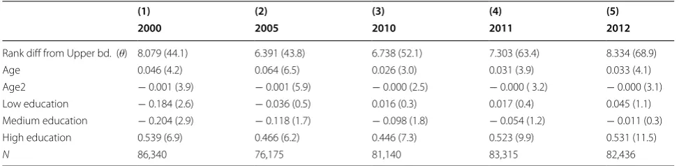
Figure 4 provides local linear regression estimates
on the relationship between the full-time weights and
the rank difference θtsi as further plausibility check. For
wages close to the upper bound (a rank difference close to zero) the weights are close to one, indicating that the (2)
ft_weighttsi=min
Pr(pt2012i =0|θtsi,xtsi)
Pr(pttsi=0|θtsi,xtsi)
, 1
=min
1−Pr(pt2012i=1|θtsi,xtsi)
1−Pr(pttsi=1|θtsi,xtsi)
, 1
. Table 1 Probit regression for part‑time spell reported, men
Probit regressions for different years (columns). t statistics in parentheses. rank diff from upper bd. ( θ ) rank difference between the rank of the individual’s own wage and the rank of the upper bound for correction, θtsi=0.88−Ft_f(wagetsi) (see Sect. 3). low education intermediate high school degree after ten years, medium
education high school degree after at least twelve years or a vocational degree, high education college degree. The regression also includes ten dummies for different occupation categories, 13 dummies for different industries, and ten dummies for the West German states. The reference category involves observations with missing values for education, occupation, industries, and states. The employment spells are weighted by their length
(1) (2) (3) (4) (5)
2000 2005 2010 2011 2012
Rank diff from Upper bd. ( θ) 8.079 (44.1) 6.391 (43.8) 6.738 (52.1) 7.303 (63.4) 8.334 (68.9)
Age 0.046 (4.2) 0.064 (6.5) 0.026 (3.0) 0.031 (3.9) 0.033 (4.1)
Age2 − 0.001 (3.9) − 0.001 (5.9) − 0.000 (2.5) − 0.000 ( 3.2) − 0.000 (3.1)
Low education − 0.184 (2.6) − 0.036 (0.5) 0.016 (0.3) 0.017 (0.4) 0.045 (1.1)
Medium education − 0.204 (2.9) − 0.118 (1.7) − 0.098 (1.8) − 0.054 (1.2) − 0.011 (0.3)
High education 0.539 (6.9) 0.466 (6.2) 0.446 (7.3) 0.523 (9.9) 0.531 (11.5)
N 86,340 76,175 81,140 83,315 82,436
9 One may wonder as to whether one should also correct spells which are
2012 part-time probability and the probability of being reported full-time in the observation year are very simi-lar. The weight decreases for a growing rank difference, implying that spells with lower wages are more likely to be misreported. For both genders, the estimates for the weights cover the part of the distribution below the ini-tially defined upper bound—every spell below the 88th and 29th percentile for women and men, respectively, in the total employment sample.
For our subsequent analysis of wage inequality, we weight the spells by the product of the full-time weight in
Eq. (2) and the relative length of the spell. The resulting
spell weight becomes
where lengthtsi denotes the length of the spell in days
and ndayst the total number of days in year t, 365 or 366, respectively.
4 Trends in wage inequality before and after the correction
We now investigate whether the paramount evidence reported in the literature for rising wage inequality until 2010 among full-timers is robust against the misreport-ing of low-wage part-time employment in the raw SIAB data as full-time employment during that time period. Doing so, we revisit the evidence reported in Möller
(2016) showing that correcting the data before 2011 does
not qualitatively change the finding of a strong rise in
wage inequality among full-timers until 2010.10
(3) weighttsi=ft_weighttsi·
lengthtsi ndayst
,
Downweighting the full-time employment spells up to 2011 mainly affects wages in the lower part of the distri-bution but still also changes higher wage percentiles. This is because a reduction in the weighted shares of work-ers with low wages mechanically increases all percen-tiles up the wage distribution, an effect which goes even beyond the percentiles above the upper bounds used for the correction. However, this increase in all percentiles is not uniform across the wage distribution—in fact the increase becomes smaller further up the distribution. Thus, the correction reduces the level of wage inequal-ity and it may possibly affect the estimated trend of wage inequality.
Figure 5 shows the trends of original and corrected
percentiles of the wage (in logs) distribution for women and men from 2000 onward. The figure shows that the upward correction is stronger in the lower tail of the wage distribution and, holding the wage level constant, the correction is stronger for women than for men. The correction for men at the median and the 25th percentile is small but still visible and it becomes sizeable at the 5th percentile for men. For women, the correction is sizeable even at the median and it grows further moving down the wage distribution. To give some numbers for 2010, the upward correction for women is 0.12 log-points (3% of the real log wage) at the 25th percentile and 0.18 log points (5%) at the 5th percentile. For men, it is 0.01 log-points (0.3%) at the 25th percentile and 0.04 log points (1.0%) at the 5th percentile. As intended, the correction smoothes the discontinuous development of the lower percentiles between 2010 and 2012. Even though the correction is stronger before 2011, the findings indicate a need for Table 2 Probit regression for part‑time spell reported, women
Probit regressions for different years (columns). t statistics in parentheses. rank diff from upper bd. ( θ ) rank difference between the rank of the individual’s own wage
and the rank of the upper bound for correction, θtsi=0.29−Ft_m(wagetsi) (see Sect. 3). low education intermediate high school degree after ten years, medium education high school degree after at least twelve years or a vocational degree, high education college degree. The regression also includes ten dummies for different occupation categories, 13 dummies for different industries, and ten dummies for the West German states. The reference category involves observations with missing values for education, occupation, industries, and states. The employment spells are weighted by their length
(1) (2) (3) (4) (5)
2000 2005 2010 2011 2012
Rank diff from Upper bd. ( θ) 2.814 (146.8) 2.558 (135.2) 2.355 (133.6) 2.804 (156.4) 3.061 (163.4)
Age 0.224 (45.8) 0.220 (46.6) 0.197 (44.4) 0.218 (49.6) 0.229 (52.0)
Age2 − 0.002 (39.8) − 0.002 (40.1) − 0.002 (37.3) − 0.002 (42.3) − 0.002 (44.1)
Low education − 0.009 (0.2) 0.017 (0.3) 0.090 (2.0) 0.109 (2.6) 0.075 (1.9)
Medium education − 0.027 (0.6) 0.005 (0.1) 0.067 (1.6) 0.209 (5.1) 0.153 (4.0)
High education 0.382 (7.8) 0.341 (6.5) 0.327 (7.3) 0.511 (11.9) 0.497 (12.3)
N 155,868 142,906 158,310 164,041 166,134
10 Recall that our analysis is restricted to West Germany whereas Möller
correction in 2011, the year of the break in the
part-time indicator.11
Clearly, the correction reduces the gap between differ-ent percdiffer-entiles, which means that it reduces the meas-ured wage inequality until 2011 compared to the original
data. Despite this, the graphical evidence in Fig. 5
sug-gests that the corrected percentiles and the percentiles based on the raw data seem to show quite similar trends
up to 2010. Figures 6 and 7 illustrate both points,
show-ing time trends for the difference between different percentiles of log wages. Wage inequality for females is higher in the lower half of the distribution, because the difference between the 50th and 20th percentile is larger than the one between the 80th and the 50th percentile. The full-time correction has its strongest effect on the
former as shown in Fig. 6. Based on Fig. 7, the
correc-tion for men is small in comparison and the difference
in the upper half of the distribution is larger than in the
lower half. Figures 8 and 9 provide a more detailed view
on wage trends by showing the cumulative growth since 2000 (measured as log differences) of wages at different percentiles.
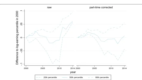
In contrast to the period until 2010, the trend in wage inequality between 2010 and 2014 is strongly affected by our correction. Based on the raw uncorrected data, one would be inclined to conclude that wage inequal-ity among women decreases strongly between 2010 and 2014 (e.g. the 80–20 gap decreases by about 10 log points,
Figs. 6 and 8 to the left) and it levels off for men (Figs. 7
and 9 to the left). After the correction, wage inequality for
both genders levels off and, especially in the lower part of the wage distribution, there is less real wage growth after
2010 (Figs. 8 and 9 to the right).
As final part of our empirical analysis, we investigate the age dimension of wage inequality. Antonczyk et al.
(2018) find that an important aspect of the rise of wage
inequality among men was that wage differences between older and younger workers increase strongly until 2004 and that real wages fell strongly for younger workers, especially in the lower part of wage distribution. Against this backdrop, we contrast workers aged 25 to 34 and those aged 35 to 55. Specifically, we investigate whether wage trends for younger workers at the bottom of the wage distribution continued to fall strongly after 2004
.8
5
.9
.9
5
1
full-time weight
0 .2 .4 .6 .8
theta
Women Men
Fig. 4 Local linear regression for the full-time weight. Estimates for a local linear regression of the full-time weight on the rank difference θ . For
individual percentile ranks close to the upper bound until we correct, θ approaches zero. θ is the larger the lower the rank in the wage distribution.
For women and men, only the part below the respective upper bound, 88th and 29 percentile, is considered for the correction
11 However, the implied trends of wage percentiles for the corrected data are
5th percentile, men
5th percentile, women 25th percentile, men
25th percentile, women 50th percentile, men
50th percentile, women
3.5
4
4.5
5
log-earnings
2000 2005 2010 2014
year Solid Line: Raw data, weighted by the length of spell Dashed Line: Part-time corrected
Fig. 5 Percentiles of log-wage distribution, full-time, raw and corrected. Percentiles of the log-wage distribution for full-time employees, inflation adjusted, only former West-Germany (without Berlin), only employees aged 25 to 55, without marginally employed and apprentices, weighted by the length of employment spells
.2
.4
.6
.8
1
Differences in log-earning percentiles
2000 2005 2010 2014
year
difference p80-p50 difference p50-p20 difference p80-p20
p80-p50, corrected p50-p20, corrected p80-p20, corrected
.2
.4
.6
.8
Differences in log-earning percentile
s
2000 2005 2010 2014
year
difference p80-p50 difference p50-p20 difference p80-p20 p80-p50, corrected p50-p20, corrected p80-p20, corrected
Fig. 7 Percentile differences of log-wage distribution for men, full-time, raw and corrected. Differences between the 80th and 50th, 50th and 20th and 80th and 20th percentile of the log-wage distribution for full-time employees, inflation adjusted, only former West-Germany (without Berlin), only employees aged 25 to 55, without marginally employed and apprentices, weighted by the length of employment spells
-.1
-.05
0
.0
5
.1
2000 2005 2010 2014 2000 2005 2010 2014
raw part-time corrected
20th percentile 50th percentile 80th percentile
Difference to log-earning percentile in 2000
year
-.15
-.1
-.05
0
.0
5
.1
2000 2005 2010 2014 2000 2005 2010 2014
raw part-time corrected
20th percentile 50th percentile 80th percentile
Difference to log-earning percentile in 2000
year
Fig. 9 Cumulative real wage growth for men, full-time. Differences in log real wages over time, indexed to 0 in year 2000, only former West-Germany (without Berlin), only employees aged 25 to 55, without marginally employed and apprentices, weighted by the length of employment spells
-.1
-.05
0
.0
5
.1
2000 2005 2010 2014 2000 2005 2010 2014
raw part-time corrected
20th percentile, aged 25-34 50th percentile, aged 25-34 80th percentile, aged 25-34 20th percentile, aged 35-55 50th percentile, aged 35-55 80th percentile, aged 35-55
Difference to log-earning percentile in 2000
year
and whether there was a reversal after 2010, while check-ing whether key results change after applycheck-ing our
cor-rection. Figures 10 and 11 show the wage trends by age
groups and gender, both based on the raw data and the corrected data.
Our findings show that cumulative wage growth at all percentiles is lower for younger workers than for older workers and that wage inequality within wage groups grows strongly over time (because wage growth at lower percentiles is lower than at higher percentiles). The effects of the correction are similar to what has been dis-cussed above for the overall wage distribution. The cor-rection reduces the wage growth after 2010, especially in the lower tail of the wage distribution and for women. The key findings are that there was a very strong fall of real wages for young workers until 2010, especially at lower percentiles with the 20th percentile falling by about 10 log points for women and 17 log points for men. After 2010, there is a modest recovery of wages for both men and women except for the 20th percentiles for men in both age groups and the 20th percentile for older women. Incidentally, wages at the 20th percentile for young women grow in parallel to the other percentiles in that group. Our findings confirm the strong decline of real wages for young workers at low percentiles [as stressed
by Antonczyk et al. (2018)] for men during a longer time
period (until 2010). Further, there is little indication of a recovery after 2010. Clearly, these findings would deserve more scrutiny, which is, however, beyond the scope of this paper.
5 Conclusions
The Sample of Integrated Labor Market Biographies (SIAB) are based on German social security records which involve an indicator for part-time or full-time work. These data are widely used to analyze trends in wage inequality among full-time workers. The reporting procedure for the part-time indicator changed in 2011 with dramatic consequences on the share of reported part-time workers. This paper develops a refined cor-rection procedure for this break and investigates the robustness of previous findings on the evolution of wage inequality in Germany. We argue that the full adjustment to the new reporting procedure was completed only in 2012 and therefore we also apply our correction approach to the data for 2011.
Our correction approach involves estimating the prob-ability of being reported to work part-time as a function of the rank difference in the wage distribution among all employees (full-timers and part-timers) for all years 2000
-.2
-.15
-.1
-.05
0
.0
5
.1
2000 2005 2010 2014 2000 2005 2010 2014
raw part-time corrected
20th percentile, aged 25-34 50th percentile, aged 25-34 80th percentile, aged 25-34 20th percentile, aged 35-55 50th percentile, aged 35-55 80th percentile, aged 35-55
Difference to log-earning percentile in 2000
year
to 2012. The full-time employment data before 2012 is then reweighted using inverse probability reweighting based on the estimated propensity scores. This approach detects and downweights observations which are likely to be misreported as full-time, which results in a continu-ous upward correction of low wage percentiles among full-timers. We plan to make the correction procedure available to all users of the SIAB data.
Using our correction, the paper confirms that the rise in wage inequality among full-time workers in West Ger-many until 2010 is not a spurious consequence of the misreporting of working time. Furthermore, based on our corrected data, we find that the fall in real wages among full-timers during the 2000s was strongest among young workers and there is in fact a trend reversal after 2010, as
already observed by Möller (2016). While the raw wage
data show strong wage growth for women after 2010, the correction shows that most of this growth is spurious. In fact, based on the corrected data, wage trends between 2010 and 2014 have contributed little to reverse the strong increase in wage inequality until 2010, a findings which holds in particular for low-wage earners among men. On a methodological note, our findings show the importance of correcting for the break in the part-time indicator when analyzing wage trends.
Future research should determine whether further key results in the literature on trends in wage inequality for
West Germany (see e.g. Card et al. 2013; Biewen et al.
2018) are robust when applied to the corrected data. In
addition, it will be of great interest to extend the analy-sis beyond the year 2014. From a methodological per-spective, this will allow to estimate longer term trends for data based on the new reporting procedure fully in place since 2012. From a substantive perspective, it will be interesting to investigate the impact of the long labor market boom with continuously falling unemployment since 2010 and the introduction of the national minimum wage in 2015 on wage trends and wage inequality.
Supplementary information
Supplementary information accompanies this paper at https ://doi. org/10.1186/s1265 1-019-0265-0.
Additional file 1. Readme file on data preparation.
Additional file 2. Stata code used for data data preparation.
Acknowledgements
We are very grateful to Johannes Ludsteck, Joachim Möller, Dana Müller, and Phillip vom Berge for helpful discussions.
Authors’ contributions
BF and AS conceived the study. BF developed the reweighting procedure and AS wrote the programs and analyzed the data. Both authors decided about the different steps of the empirical analysis and wrote the manuscript. Both authors read and approved the final manuscript.
Funding
This paper is part of the project “Female Employment Patterns, Fertility, Labor Market Reforms, and Social Norms: A Dynamic Treatment Approach”, DFG project number: FI 692/14-1 and PA 2536/1-1. Financial support by the DFG is gratefully acknowledged.
Availability of data and materials
All calculations in this paper were done based in the SIAB7514, which is available at the Research data centre (RDC) of the Institute for Employment Research (IAB) and the Federal Employment Agency in Nuremberg. The SIAB7514 is described by Ganzer et al. (2017). Due to data confidentiality restrictions the data cannot be made available in a repository but researcher can access the data through the RDC. A description of the data preparation and the STATA code used are available after publication of this paper (Addi-tional files 1, 2).
Competing interests
The authors declare that they have no competing interests.
Author details
1 IAB, Humboldt University Berlin, IFS, CESifo, IZA, ROA, Nuremberg, Germany. 2 Humboldt University Berlin, Berlin, Germany. 3 IAB (Institute for Employment Research), Regensburger Straße 100, 90478 Nuremberg, Germany.
Received: 19 July 2019 Accepted: 24 October 2019
References
Antonczyk, D., DeLeire, T., Fitzenberger, B.: Polarization and rising wage ine-quality: comparing the U.S. and Germany. Econometrics 6(2), 20 (2018) Bertat, T., Dundler, A., Grimm, C., Kiewitt, J., Schomaker, C., Schridde, H., Zem-ann, C.: Neue Erhebungsinhalte “Arbeitszeit” “ausgeübte Tätigkeit” sowie “Schul- und Berufsabschluss” in der Beschäftigungsstatistik. Methoden-bericht der Statistik der BA (2013)
Biewen, M., Seckler, M.: Unions, internationalization, tasks, firms, and worker characteristics: a detailed decomposition analysis of rising wage inequal-ity in Germany. J. Econ. Inequal. (2019). https ://doi.org/10.1007/s1088 8-019-09422 -w
Biewen, M., Fitzenberger, B., de Lazzer, J.: The role of employment interruptions and part-time work for the rise in wage inequality. IZA J. Lab. Econ. 7(1), 10 (2018)
Bundesagentur für Arbeit: Schlüsselverzeichnis für die Angaben zur Tätigkeit, Ausgabe 2010. Meldeverfahren zur Sozialversicherung (2019)
Card, D., Heining, J., Kline, P.: Workplace heterogeneity and the rise of West Ger-man wage inequality. Q. J. Econ. 128(3), 967–1015 (2013)
Dustmann, C., Ludsteck, J., Schönberg, U.: Revisiting the German wage struc-ture. Q. J. Econ. 124(2), 843–881 (2009)
Frodermann, C., Müller, D., Abraham, M.: Determinanten des Wiedereinstiegs von Müttern in den Arbeitsmarkt in Vollzeit oder Teilzeit. KZfSS Kölner Zeitschrift für Soziologie und Sozialpsychologie 65(4), 645–668 (2013) Ganzer, A., Schmucker, A., vom Berge, P., Wurdack, A.: Sample of integrated labour market biographies—regional file 1975–2014 (SIAB7514). FDZ-Datenreport, IAB Nürnberg, 1/2017 (2017)
Ludsteck, J., Thomsen, U.: Imputation of the working time information for the employment register data. FDZ-Methodenreport, IAB Nürnberg, 1/2016 (2016)
Möller, J.: Lohnungleichheit—Gibt es eine Trendwende? Wirtschaftsdienst
96(1), 38–44 (2016)
Statistisches Bundesamt.: Verbraucherpreisindizes für Deutschland. Jahresber-icht 2017 (2018)
Publisher’s Note