R E S E A R C H
Open Access
Reachability-based model reduction for
Markov decision process
Felipe M Santos
*, Leliane N Barros and Felipe W Trevizan
Abstract
This paper presents how to improve model reduction for Markov decision process (MDP), a technique that generates equivalent MDPs that can be smaller than the original MDP. In order to improve the current state-of-the-art, we take advantage of the information about the initial state of the environment. Given this initial state information, we perform a reachability analysis and then employ model reduction techniques to the reachable space of the original problem. Further, we also eliminate redundancies in the original MDP in order to speed up the model reduction phase. We also contribute by empirically comparing our technique against state-of-the-art model reduction
techniques and MDP solvers that do not perform model reduction. The results show that our approach dominates the current model reduction algorithms and outperforms general MDP solvers indenseproblems, i.e., problems in which actions have many probabilistic outcomes.
Keywords: Probabilistic planning; Markov decision process; Model reduction; Stochastic bisimulation
Background
One of the biggest challenges in the probabilistic plan-ning is to solve largeMarkov decision processes (MDPs) [1]. This is because the number of states in an MDP grows exponentially with the number of state variables, a problem known as the Bellman’s curse of dimension-ality[1]. Many techniques have been proposed to avoid the complete enumeration of states, e.g., by exploiting the structure of factored models [2, 3] and by using the infor-mation of the initial state to find the states relevant for the optimal solution by focusing on them [4, 5].
Another approach is to applymodel reductionto obtain a smaller MDP and then solve it using an off-the-shelf MDP solver [6]. In order to find the optimal solution for the original MDP, both the original and reduced MDP must be equivalent. Therefore, the problem of finding an equivalent and reduced MDP consists of computing a partitionP of the original MDP state spaceS, such that each block represents a subsetBi ⊆ Sthat groups equiv-alent states according to their reward and probabilistic transition functions.
*Correspondence: [email protected]
Institute of Mathematics and Statistics - University of São Paulo, Rua do Matão, 1010 São Paulo, Brazil
This paper extends the algorithms for computing stochastic bisimulation in two directions: reachability analysisandpartition elimination. In the former, we use the MDP’s initial state to find all the states relevant to the optimal solution and consider only this subspace of the original problem when applying model reduction. In the latter, we detect and delete intermediary partitions of the original MDP that are repeated, thus speeding up the con-vergence to a stochastic bisimulation. We also contribute with an empirical comparison among: the state-of-the-art model reduction algorithms and MDP solvers (that do not perform model reduction). The results show that our approach dominates the current model reduction algo-rithms in all problems, specially insparsedomain prob-lems where reachability analysis prunes a significant part of the state space. The experiments also show that our technique outperforms general MDPs solvers (that do not perform model reduction) indenseproblems, i.e., prob-lems in which actions have many probabilistic outcomes. This is true specially when the domain suffer a significant reduction. This happens because stochastic bisimulations withpartition eliminationcan summarize the dynamics of the domain and generate equivalent problems with half of the original MDP size.
The paper is organized as follows. The “Background” section presents our notation, background related to
MDPs, and algorithms to solve them. The “Aggregation algorithms” section presents the concepts of state aggre-gation algorithms and stochastic bisimulation, as well as the basic algorithm to compute them. The “Stochastic bisimulation over the reachable states” section contains our contributions to algorithms that compute stochas-tic bisimulations. The section “Results and discussion” empirically compares our technique combined with traditional planners against traditional model reduc-tion algorithms and planners that do not employ model reduction. Finally, the “Conclusions” section presents our conclusions.
Markov decision processes
An infinite-horizon MDP [1] is a tupleM=(S,A,P,R,γ ), where:
• S is a finite set of states that can be observed in different moments in time;
• A is a finite set of actions andA(s)⊆Ais the set of applicable actions in the states;
• P:S×A×Sis the transition function and is given byP(s|s,a)that defines the probability to reach
s∈Safter applying an actiona∈Ains∈S.P(·|·,a)
defines a probabilistic transition matrix where each row represents a states, each column represents a statesand an entry(s,s)has the probabilityP(s|s,a). We say that the transition matrix isdense if at least 50 % of the entries have probabilities greater than 0; otherwise, we called it asparse transition matrix; • R:S×Ais the reward function that represents the
reward received after applying an actiona∈Ain the states∈S; and
• γ ∈] 0, 1[is the discount factor used for weighting future rewards [1].
A solution of an MDP is apolicyπ :S →Athat maps each states∈Sto an actiona∈A.
The expected accumulated reward obtained when fol-lowing a policyπ from a statesis represented as Vπ(s) and is the fixed-point solution for the following system of equations:
Vπ(s)=R(s,π(s))+γ s∈S
P(s|s,π(s))Vπ(s), ∀s∈S.
(1)
A policyπ∗is optimal if, for every policyπands ∈S, Vπ(s) ≤ Vπ∗(s). Notice that π∗ might not be unique; however, the optimal expected accumulated reward from a state s, denoted by V∗(s), is unique [7]. The value function V∗ can be computed directly by finding the
fixed-point solution of the Bellman equations, i.e., the following system of equations:
V∗(s)=max a∈A
R(s,a)+γ s∈S
P(s|s,a)V∗(s)
, ∀s∈S.
(2)
An MDPM = (S,A,P,R,γ )is enumerative if all ele-ments of all sets that constitute the MDP are explicitly enumerated, e.g., state space S and probability tables P are represented directly by enumerating each element of them. Alternatively, an MDP can be represented in a factored form based on a set of state variables X =
{X1,. . .,Xn}. Each state is represented as a vector x = (x1,. . .,xn)of assignments where eachxi is either 0 or 1 to denote if the state variableXiis active or not. Thus, the size of the set of states in a factored MDP is 2n.
The transition function of a factored MDP is repre-sented by a set ofdynamic Bayesian networks (DBNs)[8], one for each action. A DBN for an actionais an acyclic directed graph that has the following two layers: (i) a layer representing the setXof state variables in the current state and (ii) a layer representing the setXof state variables in the next state. Every arc in a DBN representing an action is from the layerXtoXand represents the dependencies between state variables under an actiona. Given a vari-ableXj, theparentsofXj(denoted by parents(Xj)) are all variableXisuch that there exists an arc fromXitoXj.
A DBN also contains theconditional probability tables (CPTs)that give us the probability of a state variable Xj being true or false given the parents ofXj. The advantage of using DBNs is that we do not need to enumerate all pos-sible combinations of state variable values to represent the transition function. Instead, it is obtained as follows:
P(x|x,a)= n
i=1
P(xi|parents(Xj),a). (3)
An efficient way to represent the CPTs (and factored reward functions) is throughalgebraic decision diagram (ADD)[9]. ADDs extendbinary decision diagrams (BDDs) [10]. BDDs are decision trees represented in a more com-pact way in order to efficiently define functions with binary variables to a binary result, i.e.,f :Bn →B. ADDs are used to represent functions that map binary variables to real values, i.e.,f :Bn→R. Thus, to solve an MDP, we can also represent the value function as an ADD. There are ADD libraries to efficiently compute operations such as addition (⊕), multiplication (⊗), and marginalization
xi∈Xi
Algorithms for solving MDPs
Value iteration and topological value iteration
Thevalue iteration (VI)algorithm [1] uses dynamic pro-gramming in order to find V∗. Formally, VI solves the following recursive equations, wheret is the number of stages-to-go:
Vt(s)=
any value ift=0
maxa∈A R(s,a)+γ
s∈S P(s|s,a)Vt−1(s)
otherwise.
(4)
The algorithm converges to V∗ when the maximum error between the last two iterations is less than a small constant, for all states∈S. This is expressed as:
max s∈S |V
t(s)−Vt−1(s)| ≤. (5)
VI can take a long time to converge because it needs to update the values of the complete set of statesS in each iteration independently of the problem structure.
Topological value iteration (TVI)[11], an extension of VI, exploits the topological structure of the transition graph to speed up the convergence time by decreasing the number of updates performed.
Formally, TVI pre-processes the given MDP by per-forming a topological analysis of the graph representing the MDP, i.e., a graph in which the nodes are states and the arcs are actions. The result of this analysis is a set of the strongly connected components (SCCs)and TVI applies VI on each SCC in reversed topological order. This decom-position can speed up the convergence toV∗ when the original MDP can be decomposed into several SCCs with similar size. In the worst case, when the MDP has only one SCC, TVI performs worst than VI due to the overhead of the topological analysis.
Labeled real-time dynamic programming
Stochastic shortest path problem (SSP) [7] is another model for probabilistic planning. The main differences between SSPs and infinite-horizon MDPs is that SSPs contain the information about the initial state of the environment as well as a set of goal states represent-ing the stop criterion of the agent. Formally, an SSP is a tuple(S,s0,G,A,P,C)where:
• as in the MDPs,S, A, and P are the set of states, set of actions, and transition function respectively;
• s0∈Sis the initial state;
• G⊂Sis the non-empty set of goal states; and • C:S×Arepresents the cost of applying actiona∈A
in the states∈S.
SSPs are relevant for this work because any infinite-horizon MDP can be perfectly represented as an SSP [12, Section 7.3], thus we can also use algorithms devel-oped for SSPs to solve the problems presented in this paper.
One example of algorithm for solving SSPs isreal-time dynamic programming(RTDP) [4] that, given an SSP and a lower bound forV∗, computes an optimal policy for all therelevant states, i.e., all states reachable by the optimal policy starting froms0. RTDP starts froms0and visits the set of states following a greedy policy until a goal state is reached. This procedure is known as a trial and, for the case of infinite-horizon MDPs converted to SSPs, a trial can be seen as an infinite process that randomly fin-ishes with probability 1−γ every time a state is visited. RTDP performs trials until it has converged to the optimal solution.
In each state s visited in a trial, RTDP computes the greedy policy ins(the action that maximizes Equation 4), updatesVt(s), and samples a next state to be visited based on the probability distribution of the greedy action. Due to this sampling procedure, states with a low probability are updated less often than states with a higher probability, resulting in overall lower convergence.
Labeled RTDP (LRTDP) [5] is an algorithm that enhances RTDP providing a faster convergence of the optimal solution. This performance improvement is obtained by labeling the states that have already converged and finishes the trials when a converged state or goal is reached. LRTDP uses the procedureCheckSolved[5] that is responsible to decide if a state is converged or not. This decision is done based on the concept ofgreedy graph of a state s, i.e., the graph that contains all reachable states fromsfollowing the greedy policy. The optimal solution is obtained when all states in the greedy graph ofs0are marked as converged.
Aggregation algorithms
Given an MDPM, an optimal policy forMcan be found by using VI, TVI, or LRTDP. Another way to find an opti-mal policy is based on two steps: (1) getting an equivalent model of reduced size based on the original MDP and (2) solving the reduced model and applying the solution in the original MDP. The first step is known asstate aggregation for MDPs[13].
Mathematically, state aggregation algorithms for MDPs receive as input an MDPM=(S,A,P,R,γ )and computes a reduced MDPM = (S,A,P,R,γ )with a set of states Sthat groups states into blocks of states, calledabstract statesinM. It is desirable that: the set of states ofMbe much smaller than the set of states ofM, i.e.,|S| |S| and an optimal solution forMto also be optimal forM.
• Stochastic bisimulations (exact/approximate) [6, 14], a technique that receives an MDP (factored or enumerative) and returns an enumerative MDP (or a bounded-parameter MDP [15], i.e., an MDP whose functions are given by intervals);
• Homomorphisms (exact/approximate) [16, 17], techniques that are similar to stochastic
bisimulations, but can achieve greater reductions in some special scenarios;
• Structured policy iteration (SPI) [18], one of the first techniques to use decision trees to solve factored MDPs;
• Stochastic planning using decision diagrams
(SPUDD) [2], a technique that is a factored version of value iteration. This was the first algorithm that used ADDs to solve MDPs more efficiently; and
• Symbolic real-time dynamic programming - sRTDP
[3], a factored version of RTDP that also uses decision diagrams.
A complete overview about state aggregation algorithms is presented in [13]. Some of these algorithms are com-pletely factored, that is, they never use the concept of enumerative states set. At the same time, others can com-bine factored and enumerative representations. We chose exact stochastic bisimulations because with them, we can easily compare time and reduction performance against exact enumerative MDP planners. Moreover, we do not need to define a criterion to compare different approx-imate solutions because the exact solutions are unique. Thus, from now on, we will consider that model reduc-tion and model minimizareduc-tion are algorithms that compute exact stochastic bisimulations.
The state aggregation algorithms for MDPs usually work based on the concept of partitions. Apartitionof a setS is a set of disjoint subsets whose union is S itself. Each disjoint subset can also be called ablock. Given an enu-merative MDPMand a set of statesS, a partition overSis given byP = {B1,. . .,Bk}, wherePis a partition ofSand eachBi∈ {1,. . .,k}is a block.
Two important concepts for model reduction are refine-ment andcoarsening of a partition. A partition P is a refinement of a partitionPif and only if each block ofPis a subset of some block inP, i.e., a refinement splits a block Bi in sub-blocks generating a finer partition. IfP = P, Pstill is a refinement ofP. The concept of coarsening is opposite to the concept of refinement: ifPis a refinement ofP,Pis a coarsening ofP[6].
Definition 1. Given thatP1andP2are partitions ofS described by enumerative states, we can generate a par-tition P3 that is a refinement of P1 and P2 with the intersection of them, i.e.,P3 = P1∩P2such that each Bk ∈ P3 is computed by the intersection of two blocks
Bi ∈P1andBj∈P2, withBi∩Bj = ∅. To compute every Bk ∈P3, it is necessary to do all combinations ofBi∩Bj.
If we use factored representation instead of enumer-ative representation, it is possible to get more efficient algorithms for performing model reduction [6]. Hence, let X = {X1,. . .,Xn}be the set of state variables of a given factored MDP andS⊆2na set of valid states of this MDP. A block of states can be characterized by adisjunctive nor-mal form (DNF)expression over the boolean variables in X, i.e.,Bican be represented as a boolean formula and we use a labelvi to identify the block. Thus, alabeled par-tition ofS is a setP = {(B1,v1),. . .,(Bk,vk)}such that (ki=1Bi) =S. Furthermore, asPis a an augmented par-tition, each pairvi,vjassociated with blocksBi,Bjmust be different and unique in the partition. Each(Bi,vi)∈Pis a tuple with a partition blockBiand an unique labelvithat is common to alls∈Bi. For instance,P= {(X1, 2),(¬X1, 3)} is a labeled partition with two blocks: a block of states, labeled with 2, whereX1is satisfied and a block of states, labeled with 3, where¬X1is satisfied.
Definition 2.Given thatP1andP2 are labeled parti-tions ofSdescribed by DNF expressions, we can generate a partitionP3that is a refinement ofP1andP2with the intersection of them, i.e.,P3=P1∩P2whereBk ∈P3is computed by the conjunction (∧) of two blocksBi ∈ P1, Bj ∈ P2 such that Bi and Bj are not mutually exclu-sive DNF expressions of the kindX1∧ ¬X1. To compute every Bk ∈ P3, it is necessary to compute all combina-tions of conjunccombina-tions considering different possibilities of Bi∩Bj. The labelvk must be different from the labelsvi andvj. By definition, a partition ofSwith a single block is represented by the boolean expressiontrue.
For example, given the partitions (Fig. 1)P1= {(X1, 2), (¬X1, 3)} and P2 = {(X2 ∧ X3, 5),(X2 ∧ ¬X3, 7), (¬X2, 11)}, their intersection will result in the refined par-tition P3 = {(X1 ∧X2 ∧X3, 10), (X1∧X2∧ ¬X3, 14), (X1∧ ¬X2, 22),(¬X1∧X2∧X3, 15),(¬X1∧X2∧ ¬X3, 21), (¬X1∧ ¬X2, 33)}. In general, givenmpartitionsP1, . . . , Pm, it is possible to get a refinement by computing the intersection of them asP=mi=1Pi[6].
Figure 2 shows a sequence of refinements. In the begin-ning of the first iteration, it is given a partition with a single block. After the first iteration of refinements, the partition is split into two blocks. In the next two iterations, we get partitions of two and three blocks, respectively. Finally, a new refinement is done and the partition does not change. Hence, it is not necessary to split more blocks. From this example, we could extract an MDP M with
|S| =5.
Fig. 1Refinement of partitions. Refinement of partitionsP1with two blocks andP2, with three blocks. The refinement result is given byP1∩P2,
a partition with six blocks
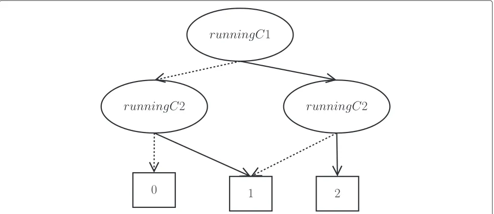
the same reward or transition probability. For example, consider the domainSysadmin, where we haven comput-ers that must be running. Given a problem (instance) of this domain, we can apply the actions rebootCior noop at each stage of the MDP. In an instance with two comput-ers:C1 and C2, we have two state variables: runningC1 and runningC2 and three actions: noop, rebootC1 and rebootC2. The reward function for the action noop, given as an ADD, can be viewed in Fig. 3. For instance, if we execute the noop action in the state where runningC1 is true and runningC2 is false, the reward is 1. To refer to the partitions of an MDP, we use a special notation: for each actiona ∈ A, we have a partitionPRawith respect to the reward function; and for each pair of actiona ∈ Aand state variableXi ∈ Xthat can be changed bya, we have a partitionPXaiwith respect to the factored probabilistic transition function.
The partition obtained from the reward func-tion in Fig. 4 is implicitly represented as PRnoop =
{(B1,v1),(B2,v2),(B3,v3)}, where: B1 = {runningC1 ∧ runningC2}, with reward 2; B2 = {(¬runningC1 ∧ runningC2)∨(runningC1∧ ¬runningC2)}, with reward 1; andB3= {¬runningC1∧ ¬runningC2}, with reward 0. We can do the same for the other actions generating the partitions:PrebootC1R andPrebootC2R .
The partitions obtained from the factored probabilistic transition functions, for theSysadminexample, for each pair of action and state variable are:PrunningC1noop ,PrunningC2noop ,
PrebootC1
runningC1,PrunningC2rebootC1 ,PrunningC1rebootC2 andPrunningC2rebootC2 . Thus, in general, the maximum number of different partitions we can have is|A| +(|A| × |X|), where|A|comes from the reward function of each action and|A| × |X|comes from the factored probabilistic transition functions considering each pair of action and state variable.
A labeled partition can be represented using an ADD where each leaf represents an unique labelvi. The DNF
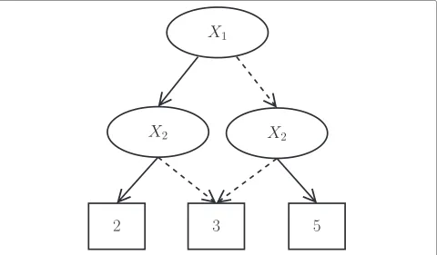
expression that characterizes a block of statesBiis given by the disjunction of the conjunctions among state vari-ables, obtained from different paths that go from the ADD root to the leaf labeled withvi. For instance, Fig. 5 shows an ADD that represents the following labeled partition:
P = {(X1∧X2, 2),(X1∧ ¬X2, 3)∨(¬X1∧ ¬X2, 3), (¬X1∧X2, 5)}
To compute the refinement ofqlabeled partitions rep-resented as ADDs, we need to get the product of ADDs representing these partitions. Note that performing the product of ADDs representing partitions is the same of computing the intersection of the partitions [6]. In this case, we need to define unique labels for them that will also be unique after the product is computed. For this purpose, the blocks are labeled with prime numbers.
Figure 4 shows the ADD that represents the reward function for the actionnoopin theSysadminexample that corresponds to the tabular representation in Fig. 3. We can make a partition based on this ADD by creating a copy of it and changing the leaf values to distinct prime num-bers as in Fig. 6. Figure 7 shows an example of partition refinement showed in Fig. 1 using ADDs. To refer to the partitions represented with ADDs, we use the following notation: PRa is denoted by PDDa,R and PXa
i is denoted by
Pa,Xi
DD.
Stochastic bisimulation concepts
This section presents a technique that receives an MDP as input and computes an enumerative MDP of reduced size by searching for astochastic bisimulation[6], i.e., a partition in which states in a same block have the same behavior under any action in the MDP.
Thus, these states can be considered equal because the partition can be seen as an equivalence relation [6].
Fig. 3Reward function as a table. Reward function for action noop in an instance of the domain SysAdmin with 2 computers
Definition 3.LetP be a partition ofS. We say thatP
is a uniform partition with respect to the reward function if, for each Bi ∈ P,s,s ∈ Bi, anda ∈ A, we have that R(s,a)=R(s,a)[6].
Definition 4.Given two blocksBj ∈ P andBw ∈ P, if the following holds for alls∈Bj,s∈Bj, anda∈A
s∈Bw
P(s|s,a)= s∈Bw
P(s|s,a),
for alls∈Bj,s∈Bj, anda∈A. Then, we say that blockBj is stable with respect toBw[6].
Definition 5. A block Bj is stable if it is stable with respect to allBw∈P[6].
Definition 6. (Stochastic bisimulation) A partitionPis homogeneous ifP is uniform with respect to the reward
function and if all blocks in P are stable. We say that a partition is a stochastic bisimulation if it is homo-geneous [6].
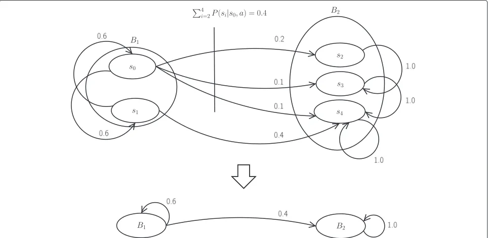
For example, consider the MDP with five states in Fig. 8 (upper). Suppose that the following conditions hold for this MDP:
• For alls∈S,A(s)=a, • R(B1,a)= −1, and • R(B2,a)=0.
Based on these conditions, we can say thatP = {B1,B2} is a homogeneous partition that results in an MDP M containing only two abstract states (Fig. 8 (lower)).
In order to find a stochastic bisimulation, we need to define an initial partition that can be a uniform parti-tion with respect to the reward funcparti-tion. After that, we
Fig. 5A partition represented as an ADD and its DNF expression. A partitionPof a set of statesSin which the blocks are represented by the set of state variablesX= {X1,X2}. The partition isP= {(X1∧X2, 2),((X1∧ ¬X2)∨(¬X1∧ ¬X2), 3),(¬X1∧X2, 5)}
need to refine the partition blocks in order to make them stable, i.e., we refine them by splitting blocks that contain states that should not be together according to the tran-sition function of these states. The process stops when all blocks are stable and the resulting partition is a stochastic bisimulation [6].
Definition 7.(Reduced enumerative MDP) Given a
partitionP that is a stochastic bisimulation, the reduced enumerative MDP [6] is defined asM =(S,A,P,R,γ ), where S is given by the blocks of P, i.e., Bi ∈ P is an abstract state belonging to S; R(Bi,a) = R(s,a) for any s ∈ Bi; and P(Bw|Bj,a) = s∈BwP(s
|s,a)
Fig. 7Refinement of partitions with ADDs. Refinement of partitionsP1andP2from Fig. 1, computed using the productP1⊗P2
for any s ∈ Bj and for all Bw ∈ P, Bj ∈ P and a∈A.
Theorem 1.Given a stochastic bisimulation P for an
MDP M and let Mbe the reduced MDP obtained fromP, then an optimal policy for Mis also optimal for M[6].
The advantage of solvingMis the possibility of doing less updates while looking for an optimal policy. For exam-ple, if s1,s5 ∈ SandBi = {s1,s5} ∈ S, we can update onlyV(Bi)instead ofV(s1)andV(s5), with the guarantee (Theorem 1) that in the optimal policy,π∗(s1)=π∗(s5)= π∗(B1).
Factored model reduction
Model reduction with factored splits (MRFS) is an algo-rithm to compute a homogeneous partition for factored MDPs [6]. MRFS can find a stochastic bisimulation using concepts of MDPs partitions combined with an opera-tion called structure-based split (SS) [6], that refines a single block Bj ∈ P with respect to a block Bw ∈ P in order to generate sub-blocks stable with respect to Bw ∈ P. The SS operation receives a block Bj ∈ P, a block Bw ∈ P and returns a partition P that is a refinement of P in which Bj is replaced by sub-blocks Bj = {B1,. . .,Bl}such that any sub-block in Bj is stable
with respect to Bw (Definition 4). This is computed as follows [6]:
SSBj,Bw,P
=P− {Bj}
∪
a∈A
BSBj,Bw,a
,
(6)
where BSBj,Bw,a=Bj∩Xi∈vars(Bw)P
a Xi
represents a block split considering one action and vars(Bw) is the set of state variables used to represent blockBw[6]. When BS(Bj,Bw,a)is done, we have a partition of blockBjthat is stable with respect toBwconsidering only actiona. To have Bj stable with respect toBw, SS calls BS for each actiona ∈ Aand compute the intersection of the resul-tant partitions. The usage of vars(Bw)instead of all state variables in Xis a way to efficiently compute the parti-tions, ignoring variables that will not affect the transition to blockBw.
With SS, model reduction does not enumerate all states explicitly while refining blocks, since the splits are done using only the state variables in vars(Bw)to refine a block Bj with respect to a block Bw [6]. MRFS works as fol-lows. The process starts with a uniform partition with respect to the reward function. After that, while the cur-rent partition P contains a pair of blocks Bj,Bw ∈ P such thatBj is not stable with respect toBw, the process calls SS using Bj and Bw as parameters. In the refined partition, the sub-blocks ofBjare stable with respect to Bw[6].
MRFS can also be computed with ADDs [19] by gener-ating a partition for each MDP function and refine them. To do this efficiently, we can ignore some of these parti-tions considering that in the factored MDP structure, we can have state variables that are irrelevant to model reduc-tion [20]. Thus, model reducreduc-tion can consider only the essential state variables, namedXe. One way to compute Xeis to add the state variables inPRAtoXeand, after that, recursively add the parents of those variables looking for
the factored MDP DBNs [20]. Using the set Xe, we can compute MRFS with ADDs as follows:
PDD=PDDA,R⊗PDDA,Xe, (7)
where PDDA,R = a∈APDDa,R and PA,Xe
DD =
a∈A
Xi∈XeP
a,Xi
DD
.
Methods
In the next sections we present the techniques that we use to improve model reduction performance.
Stochastic bisimulation over the reachable states
Suppose we have an MDP in which there is initial state information, that is, an MDP where we know a given initial states0 ∈ S. MRFS can be improved if we use the reach-able states information given s0, specially in problems that have sparse transition matrixes, i.e., where the set of reachable states can be much smaller than the complete set of states.
LetSreachable|s0 be the set of reachable states givens0. If this set is computed before we look for a stochastic bisimulation, it is possible to get a reachability parti-tionPDDS|s0 = Breachable|s0, 1
,B¬reachable|s0, 0
, in which Breachable|s0 represents the block of reachable states given s0
Sreachable|s0
and B¬reachable|s0 represents the block of unreachable states givens0S\Sreachable|s0
.
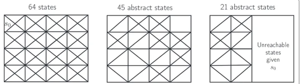
Figure 9 summarizes three different kinds of partitions that could be done over a set of statesS:
(a) a partition in which the states inS are divided into |S|blocks, i.e., each block contains a single state; (b) a partition overS in which each block can contain
more than one state; and
(c) a partition overS that has refinements only in the subsetSreachable|s0.
If we consider only partitions of item (c) to com-pute stochastic bisimulations, we can have the following advantages:
• model reduction begins with smaller partitions, what makes computing more efficient; and
• the reduced model can be smaller than (b).
To find PS|s0
DD, it is necessary to visit all the reachable states givens0. This procedure is done layer by layer, sim-ulating each action of the MDP in each reachable state (similarly to a breadth-first search [21]). Reachable states can be efficiently computed representing the sets of states in each layer as BDDs [22] and using BDD operations such as union, intersection, and marginalization. Algorithm 1 shows how we compute the reachable states given an MDP Mand a states0.
Algorithm 1:GetReachabilityPartition (M,s0)
Input:M: a factored MDP,s0: an initial state represented in the factored way
Output:PS|s0
DD: a reachability partition. PS|s0
DD ← {0}; PS|s0
DDprev← {0};
CurrentLayerDD← {0};
CurrentLayerDD←CurrentLayerDD∪ {s0→1};
whiletruedo
NextLayerDD← ∅; PS|s0
DDprev ←P
S|s0 DD;
foreacha∈Ado
ifNextLayerDD= ∅then
// Consider that GetSuccessorsByAction do what it is proposed to do and;
// return a new layer of DD.; NextLayerDD←
GetSuccessorsByAction(CurrentLayerDD,a);
end else
NextLayerByActionDD←
GetSuccessorsByAction(CurrentLayerDD,a);
NextLayerDD←
NextLayerDD∪NextLayerByActionDD;
end end PS|s0
DD ←P
S|s0
DD ∪NextLayerDD;
ifPDDS|s0prev=PDDS|s0 then
break;
end
CurrentLayerDD←NextLayerDD;
end
returnPDDS|s0;
Reachability-based model reduction
Reachability-based MRFS (ReachMRFS) is an extended version of MRFS that computes stochastic bisimulations over Sreachable|s0. Hence, it is required to compute first the reachability partition,PS|s0
DD (Algorithm 1), and after that, we compute MRFS considering only the states in Breachable|s0.
The algorithm ReachMRFS (Algorithm 2) works as fol-lows. In the first external foreach, partitions PDDa,R are multiplied by the partitionPS|s0
DD, resulting in the partitions Qa,R
DD (i.e., partitions based on the reward function for an actionaover the reachability partition), where unreach-able states are labeled with 0. As reachability partition has only two blocks, labeled with the values 0 and 1, when we compute the product of this partition with other MDP partitions, some leaves get the value 0 and others stay the same. In this way, many leaves can receive a value 0, which reduces the number of leaves and enables us to have a more compact representation. Furthermore, if we com-pute the refinements among partitions that were already simplified, the number of blocks in the refined partition is smaller than the number of partitions using all the pos-sible states. The partitions Qa,RDD are used to compute a uniform partition with respect to the reward function (i.e., for all action a ∈ A) over Sreachable, that we call PA,R
DD.
Algorithm 2:ReachMRFS(M,PS|s0 DD,Xe)
Input:M: a factored MDP;PSDD|s0: a reachability partition,Xe: the essential state variables.
Output:P: a partition in which exists a stochastic bisimulation over the reachable states and 1 block that contains all the unreachable states givens0.
PA,R
DD ←1;
foreacha∈Ado
Qa,R
DD←PDDa,R⊗P S|s0 DD; PA,R
DD ←PDDA,R⊗Qa,RDD;
end PA,Xe
DD ←1;
foreacha∈Ado
Qa,Xe
DD ←1;
foreachXi∈Xedo Qa,Xe
DD ←Qa,XDDe⊗PDDa,Xi⊗P S|s0 DD;
end PA,Xe
DD ←P
A,Xe
DD ⊗Q
a,Xe
DD;
end
PDD←PDDA,R⊗P A,Xe
DD ;
In the second externalforeach, we compute a partition with stable blocks over the reachable states in the same way, by getting a simpler partitionPDDA,X. Finally, in the last two lines, we compute the stochastic bisimulation over reachable states and return it.
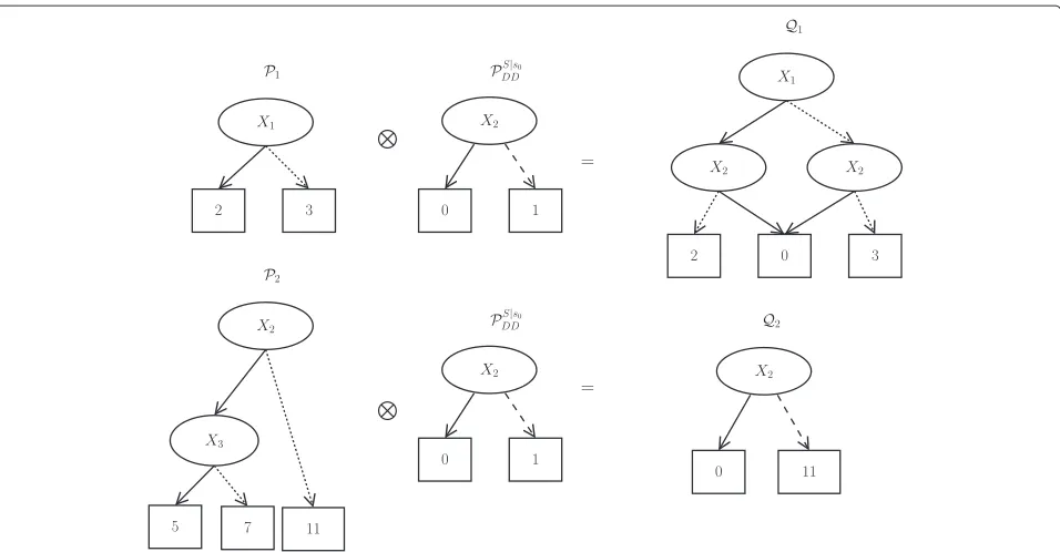
While MRFS computes the partition intersections as in Fig. 7, ReachMRFS use the reachability partition to simplify the computation. The advantages appear in two ways: (1) the program needs less space to store the ADDs in main memory and (2) the products among partitions can be done faster because many leaves are equal to 0, specially in problems with a sparse transition matrix. The benefits of ReachMRFS can be seen in Figs. 10 and 11 that shows the reduction in the size of the ADDs and hence, in the resulting partition when compared with the refinement in Fig. 7.
Reachability-based model reduction with partitions elimination
Another improvement to efficiently compute stochastic bisimulations is the elimination of repeated partitions computed by the algorithms MRFS and ReachMRFS. These algorithms use partitions based on reward and transition functions. In a general way, the maximum num-ber of distinct MDP partitions used by these algorithms is at most|A| +(|A| × |X|). However, in practical situations, these partitions are not all distinct and if we compute the stochastic bisimulation using all these partitions, the process can be very slow.
Let P and P be partitions of an MDP. We say that
P = P if|P| = |P|and if for eachB
i ∈ P there is a blockBj ∈Pwith the same DNF characterizing both of them. Based on this concept, a partitionPobtained from a functionf(reward or probabilistic transition) is repeated if the reduction algorithm found a partitionP(beforeP), obtained from a functiong(reward or probabilistic tran-sition), and we haveP = P. Given a list of partitionsL, we say the partitions are distinct among themselves if for each partitionPi ∈ Lobtained from an MDP function, Ldoes not havePjobtained from another MDP function such thatPi=Pj.
ReachMRFS-V2 (Algorithm 3) is a version of ReachM-RFS that starts computing partition elimination and then computes the refinements among the partitions inL.
Results and discussion
In [23], we have shown that ReachMRFS-V2 can be much more efficient than MRFS, specially in sparse domains. At the same time, in dense domains, the overhead of reach-ability analysis does not affect the general performance of model reduction because we use efficient ADD operations to find the reachable states. In this work, we complete those results by including VI and TVI to solve the reduced MDP. Furthermore, we also solve the original MDP M
Algorithm 3:ReachMRFS-V2 (M,PS|s0 DD,Xe)
Input:M: a factored MDP,PS|s0
DD: a reachability partition,Xe: a set of essential state variables in the MDP.
Output:P: a partition in which exists a stochastic bisimulation over the reachable states and 1 block that contains all the unreachable states givens0.
P ←1;
Pdistinct ← ∅/* initializes a map that say if a partition is repeated or not.*/;
foreacha∈Ado
Pdistinct.add(PRa→true);
foreachXi∈Xedo
Pdistinct.add(PXai →true)
end end
fori=1to|Pdistinct|do
ifPdistinct[i]=truethen
forj=i+1to|Pdistinct|do ifPdistinct[i]=Pdistinct[j]then
Pdistinct[j]←(Pdistinct[j]→false);
end end end end
L← ∅;
fori=1to|Pdistinct|do
ifPdistinct[i]=truethen L.add(Pdistinct[i]);
end end
/* Computes the refinements using the partitions in L and the reachable states in PSDD|s0. */;
foreachPi∈Ldo P ←P∩Pi∩PDDS|s0;
end returnP;
using these three algorithms to identify the trade-offs of applying model reduction.
Fig. 10Partitions over the set of reachable states givens0. The partitionsP1andP2of Fig. 7 are multiplied by the resulting partitionPDDS|s0, resulting inQ1andQ2
in Java using the official RDDL Simulator (RDDLSim) [24]. Our implementation is available in the following repository: http://github.com/felipemartinsss/repository/ tree/master/AIPlannersForRDDLSim.
The benchmark problems were taken from the Inter-national Probabilistic Planning Competition (IPPC-2011), which were specified inRDDL (Relational Dynamic Influ-ence Diagram Language)[24], a language to represent fac-tored MDPs. In the IPPC-2011, there were eight domains with ten instances each and we selected the following domains for our experiments:Crossing Traffic,Elevators, Game of Life,NavigationandSkill Teaching.
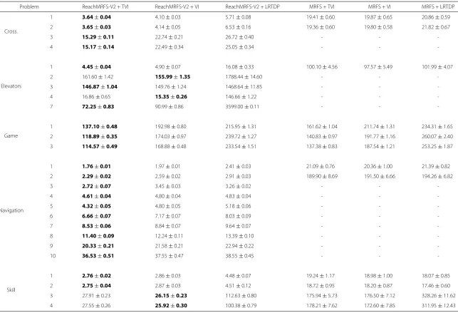
Table 1 presents the comparison between ReachMRFS-V2 and MRFS using VI, TVI, and LRTDP as planners to
solve the reduced MDP. As expected, the performance of the ReachMRFS-V2 dominates the performance of MRFS in all the problems, i.e., the slowest ReachMRFS-V2 planner (usually ReachMRFS-ReachMRFS-V2 + LRTDP) is faster than all planners that use MRFS planners. This is due the reachability analysis and partition elimination applied by ReachMRFS-V2.
Another interesting trend in Table 1 is that TVI (LRTDP) is the best (worst) planner for solving the reduced MDPs generated by both ReachMRFS-V2 and MRFS. The reason for this trend is the fact that all the states in the reduced MDPs are reachable from their initial states. Therefore, the sampling procedure of LRTDP is inefficient in comparison with the topological analysis
al.
Journal
o
ft
he
Brazilian
C
omputer
Society
(2015) 21:5
Page
13
of
16
Cross.
1 3.64±0.04 4.10±0.03 5.71±0.08 19.41±0.60 19.87±0.65 20.86±0.59
2 3.65±0.03 4.14±0.05 6.53±0.16 19.36±0.60 19.80±0.58 21.82±0.67
3 15.29±0.11 22.74±0.21 26.72±0.40 - -
-4 15.17±0.14 22.49±0.34 25.05±0.34 - -
-Elevators
1 4.45±0.04 4.90±0.07 16.08±0.33 100.10±4.56 97.57±5.49 101.99±4.07
2 161.60±1.42 155.99±1.35 1788.44±14.60 - -
-3 146.87±1.04 149.76±1.24 1468.64±11.85 - -
-4 16.86±0.65 15.35±0.26 146.66±1.22 - -
-7 72.25±0.83 90.99±0.86 3599.00±0.11 - -
-Game
1 137.10±0.48 192.98±0.80 215.95±1.31 161.62±1.04 211.74±1.31 234.31±1.65
2 118.89±0.35 174.03±0.97 239.72±1.27 140.83±0.97 191.77±1.16 260.07±2.40
3 114.57±0.49 168.88±0.48 233.54±1.51 137.38±0.83 187.54±1.21 253.25±1.87
Navigation
1 1.76±0.01 1.97±0.01 2.41±0.03 21.09±0.76 20.36±1.00 21.39±0.82
2 2.29±0.02 2.59±0.02 2.91±0.03 189.90±8.69 191.50±6.66 194.26±6.82
3 2.72±0.07 3.45±0.03 3.26±0.02 - -
-4 4.61±0.04 4.80±0.04 4.83±0.04 - -
-5 4.32±0.05 4.80±0.05 5.18±0.06 - -
-6 6.66±0.07 7.17±0.07 8.03±0.09 - -
-7 8.53±0.06 8.84±0.07 9.64±0.07 - -
-8 11.40±0.09 12.24±0.11 13.39±0.10 - -
-9 20.33±0.21 21.58±0.21 22.94±0.22 - -
-10 36.53±0.51 37.55±0.47 38.55±0.45 - -
-Skill
1 2.76±0.02 2.86±0.03 4.48±0.07 19.24±1.17 18.98±1.00 18.07±0.85
2 2.75±0.04 2.87±0.03 4.51±0.12 18.72±0.95 18.20±0.87 17.46±0.60
3 27.91±0.23 26.15±0.23 112.63±0.80 175.94±5.73 176.50±7.12 328.26±11.62
4 27.55±0.26 25.92±0.30 100.38±0.79 178.21±7.62 172.60±7.85 311.95±12.43
al.
Journal
o
ft
he
Brazilian
C
omputer
Society
(2015) 21:5
Page
14
of
16
Problem ReachMRFS-V2 + TVI ReachMRFS-V2 + VI ReachMRFS-V2 + LRTDP TVI VI LRTDP
Cross.
1 3.64±0.04 4.10±0.03 5.71±0.08 4.51±0.03 2594.45±58.66 3.16±0.05
2 3.65±0.03 4.14±0.05 6.53±0.16 4.47±0.04 2007.41±37.64 2.92±0.04
3 15.29±0.11 22.74±0.21 26.72±0.40 18.95±0.16 - 12.79±0.18
4 15.17±0.14 22.49±0.34 25.05±0.34 19.50±0.31 - 17.43,0.18
Elevators
1 4.45±0.04 4.90±0.07 16.08±0.33 5.83±0.16 135.46±3.61 13.50±0.38
2 161.60±1.42 155.99±1.35 1788.44±14.60 240.45±6.25 - 555.47±7.06
3 146.87±1.04 149.76±1.24 1468.64±11.85 217.75±5.41 - 980.74±8.64
4 16.86±0.65 15.35±0.26 146.66±1.22 14.61±0.20 1964.44±32.10 82.39±1.09
7 72.25±0.83 90.99±0.86 3599.00±0.11 78.90±1.17 208.30±3.48 1363.33±11.72
Game
1 137.10±0.48 192.98±0.80 215.95±1.31 557.46±6.35 514.48±4.60 917.27±14.06
2 118.89±0.35 174.03±0.97 239.72±1.27 440.28±5.33 399.34±3.72 1263.55±9.63
3 114.57±0.49 168.88±0.48 233.54±1.51 406.64±4.95 369.03±3.74 1399.49±7.12
Navigation
1 1.76±0.01 1.97±0.01 2.41±0.03 1.40±0.01 43.49±0.96 2.01±0.02
2 2.29±0.02 2.59±0.02 2.91±0.03 1.47±0.01 365.03±10.71 2.16±0.04
3 2.72±0.07 3.45±0.03 3.26±0.02 1.64±0.01 - 2.46±0.03
4 4.61±0.04 4.80±0.04 4.83±0.04 3.30±0.03 - 3.85±0.23
5 4.32±0.05 4.80±0.05 5.18±0.06 2.56±0.03 - 3.50±0.08
6 6.66±0.07 7.17±0.07 8.03±0.09 3.60±0.05 - 6.62±0.40
7 8.53±0.06 8.84±0.07 9.64±0.07 5.10±0.09 - 5.66±0.26
8 11.40±0.09 12.24±0.11 13.39±0.10 4.61±0.03 - 5.69±0.10
9 20.33±0.21 21.58±0.21 22.94±0.22 5.59±0.07 - 6.66±0.14
10 36.53±0.51 37.55±0.47 38.55±0.45 7.93±0.09 - 7.73±0.12
Skill
1 2.76±0.02 2.86±0.03 4.48±0.07 4.09±0.02 38.62±0.98 1.49±0.02
2 2.75±0.04 2.87±0.03 4.51±0.12 4.11±0.03 41.03±1.00 1.56±0.02
3 27.91±0.23 26.15±0.23 112.63±0.80 38.25±0.71 - 12.44±0.38
4 27.55±0.26 25.92±0.30 100.38±0.79 38.84±0.75 - 11.95±0.34
applied by TVI since no state in the reduced MDPs can be ignored.
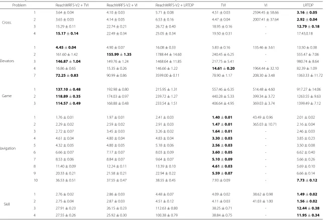
In Table 2, we compare ReachMRFS-V2 against no model reduction using VI, TVI, and LRTDP as planners.
For the Crossing Traffic domain, model reduction initially does not pay off and LRTDP has the best performance; however, as the size of the problem increases (problem #4), the reduced MDP is considerably smaller and ReachMRFS-V2 + TVI has the best overall performance.
In theElevatorsdomain, ReachMRFS-V2 + TVI is the overall best planner with ReachMRFS-V2 + VI being a closer runner-up. The reason for such performance is that the reachability analysis suffices to reduce the problem to a few thousand states. However, the reachable space con-tains only one strongly connected component, what is the worst case for TVI, therefore the overhead of the model reduction pays off when compared with TVI.
For the Game of Life domain, ReachMRFS-V2 + TVI dominates all the other planners and solve all the instances from three to ten times faster than the approaches with-out model reduction. This performance improvement is because theGame of Lifeproblems are dense and all their states are reachable. Therefore, all the reduction obtained by ReachMRFS-V2 is due to the stochastic bisimulations.
For the Navigation domain, TVI has the best perfor-mance in almost all the instances because all the model reduction is due only to the reachability analysis; there-fore, the stochastic bisimulations represent an expensive overhead.
For theSkill Teachingdomain, LRTDP dominates all the other approaches because this domain is sparse and most of the model reduction is due to the reachability analy-sis. For instance, the problem number 4 has 224possible states, only 1053 of them are reachable froms0, and the reduced model has 702 states. Therefore, the stochastic bisimulation contributes with a negligible reduction in the model.
Conclusions
The experiment results show that model reduction always pays off when we have information about the initial state. For MDPs with dense transition function, the results show that stochastic bisimulation computation can explore the domain structure and, combined with the TVI planner to solve the reduced model, can have the best performance. For instance, the Game of Life domain problems with nine variables were solved in 2–3 min with ReachMRFS-V2 + TVI (while without the reduction, LRTDP takes 15–23 min). For sparse domains likeElevatorsand Cross-ing traffic, the results show that there is an overhead of the model reduction. However, for 8 out of 26 problems, this overhead pays off and ReachMRFS-V2-based plan-ners are the best overall considered planplan-ners. It is a future
research topic to find a general rule for deciding whenever ReachMRFS-V2 should be applied or not.
Competing interests
The authors declare that they have no competing interests.
Authors’ contributions
This work is part of FMS Master thesis and LNB was his advisor. FMS carried out most of the investigation, implementation, experiments, and writing. LNB gave important ideas to the project and also contributed in the writing and revision of this manuscript. FWT gave important ideas about new techniques to solve MDPs and the implementation of the TVI algorithm and suggested a new series of experiments; he also gave an important contribution in writing and revising the paper. All authors read and approved the final manuscript.
Acknowledgements The authors would like to thank:
• CAPES, for supporting FMS during the master degree research; • FAPESP, for supporting FWT (process number 2013/11724-0); • Mijail Gamarra Holguin, for helping with the implementation of the
planners and the use of ADD library; and
• Karina Valdivia Delgado, for some ideas on factored representation and operations of MDPs.
Received: 20 May 2014 Accepted: 30 April 2015
References
1. Puterman ML (1994) Markov decision processes: discrete stochastic dynamic programming. John Wiley & Sons, New York, NY, USA 2. Hoey J, St-Aubin R, Hu A, Boutilier C (1999) SPUDD: Stochastic planning
using decision diagrams. In: Proceedings of the 15th Conference on Uncertainty in Artificial Intelligence. Morgan Kauffman, San Franciso, CA, USA. pp 279–288
3. Feng Z, Hansen EA, Zilberstein S (2003) Symbolic generalization for on-line planning. In: Proceedings of the 19th Conference on Uncertainty in Artificial Intelligence. Morgan Kaufmann, San Francisco, CA, USA. pp 109–116
4. Barto AG, Bradtke SJ, Singh SP (1993) Learning to act using real-time dynamic programming. Artif Intell 72:81–138
5. Bonet B, Geffner H (2003) Labeled RTDP: improving the convergence of real-time dynamic programming. In: Proceedings of 13th International Conference on Automated Planning and Scheduling. AAAI Press, ICAPS, Trento, Italy. pp 12–21
6. Givan R, Greig M, Dean T (2003) Equivalence notions and model minimization in Markov decision processes. Artif Intell 147:163–223 7. Bertsekas D, Tsitsiklis JN (1996) Neuro-dynamic programming. Athena
Scientific, Cambridge, MA, USA
8. Dean T, Kanazawa K (1990) A model for reasoning about persistence and causation. Comput Intell 5:142–150
9. Bahar RI, Frohm EA, Gaona CM, Hachtel GD, Macii E, Pardo A, Somenzi F (1993) Algebraic decision diagrams and their applications. In: Proceedings of the 1993 IEEE/ACM International Conference on Computer-aided Design. IEEE Computer Society Press, Los Alamitos, CA, USA. pp 188–191 10. Bryant RE (1986) Graph-based algorithms for Boolean function
manipulation. IEEE Trans Comput 35:677–691
11. Dai P, Goldsmith J (2007) Topological value iteration algorithm for Markov decision processes. In: IJCAI’07 Proceedings of the 20th International Joint Conference on Artificial Intelligence. Morgan Kauffman, San Francisco, CA, USA. pp 1860–1865
12. Bertsekas DP (1995) Dynamic programming and optimal control. Vol. 1. Athena Scientific, Cambridge, MA, USA
13. Li L, Walsh TJ, Littman ML (2006) Towards a unified theory of state abstraction for MDPs. In: Proceedings of the 9th International
Sysmposium on Artificial Intelligence and Mathematics, Fort Lauderdale, Florida, USA. pp 531–539
processes. In: Proceedings of the 13th Conference on Uncertainty in Artificial Intelligence. Morgan Kauffman, San Francisco, CA, USA. pp 124–131
15. Givan R, Leach S, Dean T (2000) Bounded-parameter Markov decision processes. Artif Intell 122:71–109
16. Ravindran B, Barto AG (2002) Model minimization in hierarchical reinforcement learning. Lecture Notes Comput Sci 2371/2002:196–211 17. Ravindran B, Barto AG (2004) Approximate homomorphisms: a framework
for non-exact minimization in Markov decision processes. In: Proceedings of the 5th International Conference on Knowledge Based Computer Systems, Hyderabad, India
18. Boutilier C, Dearden R, Goldszmidt M (1995) Exploiting structure in policy construction. In: IJCAI-95. University of British Columbia Vancouver, BC, Canada, Canada. pp 1104–1111
19. Kim KE, Dean T (2002) Solving factored MDPs with large action space using algebraic decision diagrams. In: Proceedings of the 7th Pacific Rim International Conference on Artificial Intelligence: Trends in Artificial Intelligence. Springer-Verlag, London, UK. pp 80–89
20. Guo W, Leong TY (2010) An analytic characterization of model minimization in factored Markov decision processes. In: Proceedings of the 24th AAAI Conference on Artificial Intelligence. AAAI Press, Atlanta, Georgia. pp 1077–1082
21. Russel S, Norvig P (2003) Inteligência Artificial: Uma Abordagem Moderna. Segunda edn.. Campus/Elsevier, Rio de Janeiro
22. Pednault EPD (October, 1994) ADL and the state-transition model of action. Journal of Logic and Computation, Volume 4, Number 5:1077–1082
23. dos Santos FM, de Barros LN, Holguin MG (2013) Stochastic bisimulation for mdps using reachability analysis. In: 2013 Brazilian Conference on Intelligent Systems (BRACIS), Fortaleza, Ceará, Brazil. pp 213–218 24. Sanner S (2010) Relational dynamic influence diagram language (RDDL):
language description. http://users.cecs.anu.edu.au/~ssanner/IPPC_2011/ RDDL.pdf
Submit your manuscript to a
journal and benefi t from:
7Convenient online submission
7Rigorous peer review
7Immediate publication on acceptance
7Open access: articles freely available online
7High visibility within the fi eld
7Retaining the copyright to your article