R E S E A R C H
Open Access
Tractable lithium-ion storage models for
optimizing energy systems
Fiodar Kazhamiaka
*, Catherine Rosenberg and Srinivasan Keshav
*Correspondence: fkazhami@uwaterloo.ca University of Waterloo, 200 University Ave. W, N2L 3G1 Waterloo, ON, Canada
Abstract
Model-based optimization of energy systems with batteries requires a battery model that is accurate, tractable, and easy to calibrate. Developing such a model is
challenging because electrochemical batteries exhibit complex behaviours. In this paper, we propose and evaluate a family of battery models that have different trade-offs between accuracy and complexity. We derive our models from a recently developed battery model, which is accurate and easy to calibrate but is not tractable. We evaluate our models against the commonly-used benchmark tractable model using a set of experiments that characterize the cycling behaviour of two Lithium-ion battery chemistries, as well as dynamic charge/discharge experiments. We further compare the models for two typical energy system applications, solar farm firming and grid regulation, to show the impact of the choice of battery model on the results. Finally, we evaluate the increase in accuracy when battery models are calibrated with the proper operating range.
Keywords: Battery model, Optimization, Energy
Background
The rapid decline in the cost of energy storage, particularly Lithium-ion batteries, has motivated a wide range of storage applications (Scrosati et al.2011). Many of these appli-cations, such as grid support and home energy management, require large, expensive battery systems. Hence there are many research studies being conducted on optimal bat-tery dimensioning and operation using model-based analysis of the energy system under consideration.
There exists several models which can accurately take into account the dynamic behaviour of Lithium-ion cells, including their non-linear properties such as voltage hys-teresis, efficiency losses, degradation, and temperature effects. A cell model has to be combined with a battery management system (BMS) model, which captures voltage, cur-rent, and temperature limits, to get a complete dynamic battery system model. Most of the cell models use an equivalent circuit to emulate model behaviour (see He et al. (2011); Hu et al. (2012); Chen and Rincon-Mora (2006) for examples) or complex equations to rep-resent the electrochemical interactions inside the battery (see Klein et al. (2013); Tanim et al. (2015) for examples). Some of these models are difficult to calibrate because they require data which is onerous to obtain (i.e., can only be obtained via experiments). For example, RC circuit models (Chen and Rincon-Mora2006; Hu et al.2012) require pulse charge/discharge measurements to set the resistance and capacitance parameters of the
circuit, and while there are attempts to reduce the calibration effort of these models (Ein-horn et al.2013; Hentunen et al.2014; Jackey et al.2013), calibrating them is still not an easy task. Furthermore, these models are described using complex mathematical func-tions such as differential equafunc-tions, and this makes them unsuitable for optimization studies usingmathematical programs.
The computational effort required to solve a mathematical program is proportional to the number and complexity of equations and model constraints in the program. The sim-plest programs to solve are linear programs (LP), which have reasonable solving times even when the program has hundreds of thousands of constraints (Gearhart et al.2013). The most commonly used battery model in studies requiring an optimization framework is linear (for examples, see Khalilpour and Vassallo (2016); Hassan et al. (2017); Mehra-bankhomartash et al. (2017); Atia and Yamada (2016); Chen et al. (2012)). It uses power as input, rather than current. This model, henceforth referred to as thebenchmark, uses linear and constant approximations to many of the non-linear dynamic characteristics of a Lithium-ion battery, and the loss in model accuracy as a result of these approximations is not clear. We are unaware of any published works that thoroughly evaluate the bench-mark model’s accuracy, explain how to calibrate it properly, and explore how it affects the results of the optimization studies that use it.
In this paper, we start by comparing the accuracy of the benchmark to an experimentally-validated, non-linear, and non-analytic PI model1 developed by Kazhamiaka et al. (2018) which is also based (power is conserved, and power-based models are much simpler since they do not necessarily require voltage/current transformations). To do so, we propose a calibration process for the benchmark and we find that it compares poorly with the PI model in estimating the battery energy content, which suggests that it is problematic to base battery optimization studies on this model. This finding motivates the development of new battery models with improved accuracy to replace the benchmark as the go-to model for mathemati-cal programming. Developing and validating these new models is the main focus of this paper. In this context, we aim at developing models with the following desirable properties:
1. Tractability: use only simple polynomial expressions with low degrees. The goal is to be as simple as possible to reduce the computation time, while respecting the inherent non-linearity of Lithium-ion batteries.
2. Calibration using only the data commonly found in a battery datasheet (spec), to avoid onerous experiment-based calibration and therefore make it more likely for the model to be adopted by the research community.
3. Use power as input, rather than current.
4. Integrate the constraints typically imposed by a BMS, i.e., a complete battery model, rather than a cell model.
• We evaluate the accuracy of the benchmark model and incidentally show how to calibrate it.
• We methodically extract three tractable models, one of which is linear, from the PI model and explain how to calibrate them using a spec sheet.
• We thoroughly evaluate each of them using anextensive measurement campaign on two Lithium-ion battery chemistries.
• We conduct two application studies that illustrate the effect of model complexity on the outcome of optimization analyses.
• We provide guidelines for researchers on how to choose which model to use in order to improve the accuracy of their battery system study.
The main messages of our study are the following:
• We have developed a new linear model that is more accurate and just as tractable as the benchmark model for optimization studies.
• The choice of model can significantly affect the conclusions of model-based energy system studies and that sometimes a quadratic model is necessary.
• The operating range of the battery is a crucial parameter for obtaining accurate results with simplified models.
The rest of the paper is organized as follows. In the “Existing models” section we describe the benchmark and PI models. In “A Family of Tractable Models” section, we simplify the complex aspects of the PI model to develop and calibrate a set of tractable models. In the “Evaluation” section, we compare the accuracy of the tractable models, the benchmark and the PI model. In the “Applications” section, we dimension a solar farm and a grid regulation battery application using different models to characterize the practical trade-off between the accuracy and complexity of our tractable models. We provide some practical advice on how to choose the right model for a system study In the “Discussion and Limitations” section and conclude the paper in the “Conclusion” section.
Existing models
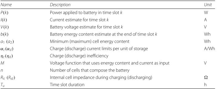
In the following, we use a discrete time model. The duration of a time slot isTuand the time index isk. Table1summarizes the notations and the corresponding units.
Table 1Notation
Name Description Unit
P(k) Power applied to battery in time slotk W
I(k) Current estimate for time slotk A
V(k) Battery voltage estimate for time slotk V
b(k) Battery energy content estimate at the end of time slotk Wh
a1(a2) Minimum (maximum) cell energy content Wh
αc(αd) Charge (discharge) current limits per unit of storage A/Wh
ηc(ηd) Charge (discharge) inefficiency
M Voltage function that uses energy content and current as input V
n Number of cells that compose the battery
Ric(Rid) Internal cell impedance during charging (discharging)
The Benchmark Model
Given the energy content,b(k−1), of a battery in time-slotk−1, and an applied power
P(k)which is constant over time slotk, the benchmark model calculates an estimate of the energy contentb(k)at the end of thekthtime slot using simple linear equations. It models three basic properties of a cell: 1) the charging and discharging inefficiencies (ηdandηc, respectively), 2) the upper and lower energy content limits (a1anda2, respectively), and 3) the charging and discharging current limits (αcandαd, respectively), which are converted into power limits by taking their product with the corresponding nominal cell voltage (Vnom,candVnom,d). The (constant) values of all these parameters can be obtained from the spec sheet of the cell. For a battery system comprised ofncells, the battery energy and power limits scale withn.
The typical formulation of the benchmark model for a battery withncells is given below. The piece-wise Eq.2is often expressed in linear form by splittingP(k)into separate charg-ing and dischargcharg-ing variables, sayc(k)andd(k)respectively. It is physically impossible for the model to charge and discharge the battery simultaneously, which yields the following non linear constraintc(k)·d(k)=0. It has been shown in Ghiassi-Farrokhfal et al. (2016) that this constraint can often be relaxed, making the model linear.
The benchmark (ncells):
b(k)=b(k−1)+E(k) (1)
E(k)=
ηcP(k)Tu :P(k)≥0 ηdP(k)Tu :P(k) <0
(2)
nαdVnom,d≤P(k)≤nαcVnom,c (3)
na1≤b(k)≤na2 (4)
Note that ηc, ηd, a1, and a2 are all constant, and the performance of the model is heavily dependent on the calibration of these parameters. However, it is com-mon practice to calibrate the model without considering the following: 1) the operating range of the application (discussed in the “Operating Range” section), and 2) all of the data typically available in a spec sheet. In most papers, the following parameters are used for lithium-ion batteries irrespective of the operating range: the discharging efficiency is equal to the charging efficiency and is in the range of 90–95%, anda1 = 0,a2 = BwhereBis a ‘nominal’ capacity. We will show that the benchmark model can be derived from the PI model, and hence the calibration procedure we propose is based on the calibration of the PI model, where parameter values are computed from spec sheet data. We discuss parameter calibration in greater detail in the “Methodology” and “Operating Range” sections.
The PI Model
The purpose of a dynamic battery model is to compute the evolution of the energy content of a battery as it is charged or discharged. However, it is extremely dif-ficult to directly measure the energy content of a battery. The PI model takes advantage of the relationship between battery voltage and current, which are easy to measure, to infer the energy content. The full formulation, calibration proce-dure, and evaluation of the PI model can be found in Kazhamiaka et al. (2018). All of our tractable models are derived from the PI model, so we describe it in detail below.
The inputs to the PI model are the applied power P(k), and the energy con-tent of the battery in the previous time step, b(k − 1). The model calculates an estimate of the resulting battery V(k), charge/discharge current I(k), and energy content b(k). It takes into account the voltage- and current-dependent charging and discharging inefficiencies (ηc(I(k)) < 1 and ηd(I(k)) > 1, respectively), the current-dependent lower and upper limits on the energy content (a1(I(k))
and a2(I(k)), respectively), as well as the charging and discharging current limits (αcandαd, respectively).
The voltage of the battery is modeled using a function M which maps the energy content and applied current to a unique battery voltage. The M function cap-tures the voltage hysteresis behaviours, where the voltage jumps relative to the open-circuit voltage (idle battery) when a charging current is applied, and drops when a discharging current is applied. The M function also captures the pro-portional change in voltage with respect to the change in the battery’s energy content.
The functions a1(.), a2(.), and M(.) and constants αc and αd are parameters to the model and can be obtained using a spec sheet.ηc(.)andηc(.)are given by Eqs.7and8 respectively. They are functions ofIandV as well as the internal impedances of a cell
Ric and Rid for charging and discharging respectively, which can also be found in a spec sheet2.
The following set of equations and constraints describes the PI model: The PI model:
b(k)=b(k−1)+E(k) (5)
E(k)=
ηc(I(k),V(k))P(k)Tu:P(k)≥0 ηd(I(k),V(k))P(k)Tu:P(k) <0
(6)
ηc(I(k),V(k))=1−I(k)Ric
nV(k) :I(k)≥0 (7)
ηd(I(k),V(k))=1−I(k)Rid
nV(k) :I(k) <0 (8)
V(k)=M(b(k),I(k)) (9)
I(k)= P(k)
V(k) (10)
nαd≤I(k)≤nαc (11)
This formulation requires the numerical computation of the intersection between the surface defined by Eq.9 in the plane(I(k),V(k)) and the surface (in the same plane) defined by the following equation (assumingP(k)≥0):
b(k)=b(k−1)+
1− I(k)Ric
nV(k)
I(k)V(k)Tu
The details of this process, as well as instructions on how to calibrate the model parameters, are documented in Kazhamiaka et al.2018.
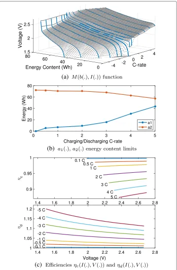
Thea1(.),a2(.),M(.),ηc(.), andηd(.)functions are shown for a Lithium-Titanate (LTO) cell (Leclanché 2014) in Fig. 1, where the current is expressed in terms of C-rate; 1 C is defined as the current which fully discharges the battery in one hour. The cell has a nominal charge capacity of 30 Ah, hence 1 C corresponds to a 30 A current. A negative C-rate is used to represent a discharging current.
A Family of Tractable Models
The PI model has three principal components: theMfunction that maps from energy content and charge/discharge current to battery voltage, the energy content limits (a1(.) anda2(.)), and the inefficiency functions (ηc(.)andηd(.)). TheM,a1, anda2functions are numerically derived from the spec sheet, i.e., they are not explicit, and this prevents the PI model from being used as part of a mathematical optimization program. The inefficiency functions are explicit but yield non-linearities and this makes the model difficult to use for mathematical optimization.
We therefore derive a set of tractable models by approximating these three components with polynomials. Our methodology is to test different combinations of approximations, starting with higher degree polynomials and working down to constant approximations, keeping combinations that show a noticeable difference in performance compared to the next iteration, and discarding those that do not have a favourable accuracy-complexity trade-off. We test each combination by simulating charge/discharge cycles at different C-rates and comparing theb(k)estimates of the model with that of the PI model to quan-tify the loss of accuracy due to the approximations. The complexity of each model is on the spectrum between the PI and benchmark models; indeed, approximating the three complex components of the PI model with constants results in the benchmark model. In developing our models, we experimented with polynomial approximations of degree less than or equal to 3.
In this section, we show how to derive the benchmark model and three novel tractable models which have a favourable accuracy-complexity trade-off.
Methodology
(a)
(b)
(c)
Fig. 1aMfunction, which maps the applied current and energy content to a unique voltage, shown with blue curves obtained from a spec and grey points representing the interpolated surface between the curves. ba1(.)anda2(.): points obtained from the spec.cηc(.)andηd(.), with each line representing the efficiency
at a different C-rate, as per Eqs.7and8
Voltage Estimate
When a battery has a certain amount of energy that can be extracted from it, and is subject to a current, this results in a certain voltage across the positive and negative electrodes. In the PI model, the voltage estimate is obtained by using theMfunction, which rep-resents the relationship between energy, current, and voltage for a given battery, and is obtained by sampling the voltage curves found in the battery’s spec sheet. To make the PI model analytical,Mhas to be expressed in analytic form. We consider the following two polynomial approximations3:
V(k)=
Vnom,d :P(k) <0 Vnom,c :P(k)≥0
(13)
V(k)=x00+x10I(k)+x01b(k) (14)
The constant approximation of the voltage corresponds to the ‘nominal’ voltage of the battery,Vnom,cwhen charging andVnom,d when discharging; these can be computed by taking the average of the voltage curves over the OR. Note that we can separate the charg-ing voltage from the dischargcharg-ing voltage (as done in Eq.13) for the linear approximation (Eq.14) without increasing the complexity of the model because of the natural separation between charging and discharging processes in Eqs.6,11, and12, but we found that this has little effect on the overall accuracy of the resulting model when applied to Eq.14.
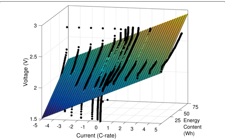
Figure2shows the non-analyticMfunction from the PI model, and the linear approx-imation given by Eq. 14 which takes the form of a plane with the best least-squares approximation of the function4over the OR. The plane is able to capture the positive slope of the voltage with increasing current and energy content, but does not capture the
rapid drop as the battery voltage approaches the lower limit. A cubic function is able to capture these dynamics, however we found that the additional complexity of the cubic function over the plane offered negligible improvements to the accuracy of the model.
Energy content limits
Energy content limits are functions of the current, and can be obtained empirically from the voltage curves in the spec sheet. We consider the following approximations toa1(.) (similarly fora2(.)):
a1(I(k))=na¯1 (15)
a1(I(k))=u1I(k)+v1n (16)
¯
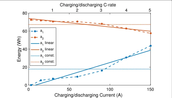
a1is computed by taking the average of thea1(.)curve over the OR, andu1andv1are parameters which define the line of best fit (least-squares) toa1(.)over the OR. In our evaluation, we found that the linear form in Eq. 16offers the best trade-off between accuracy and complexity, i.e., better approximations offered very small improvement in accuracy at the cost of much higher complexity. Figure3shows thea1(.)anda2(.) func-tions for an LTO cell, as well as their linear least-squares and constant approximafunc-tions used in our tractable models.
Charging/discharging efficiencies
In the PI model, the charging (resp. discharging) efficiency (Eqs.7,8) is a function of the voltage, current, and nominal internal resistance during charging(Ric)(resp. discharging (Rid)). The efficiency formula makes the model inherently non-linear, since bothIandV
are variables of the model and hence the equation is quadratic in terms of the variables. Furthermore, the energy content update equation (Eq.6) has a product of the efficiency and the applied power–which is the free variable in an optimization problem–to update
Fig. 3Lower(a1)and upper(a2)energy limits for an LTO cell, along with linear and constant
the battery energy content estimate. We consider the following approximations forηc (similarly forηd):
ηc= ¯ηc (17)
ηc(I(k))=1− I(k)Ri
Vnom,c
(18)
Using constant approximations for the charging(ηc)¯ and discharging(ηd¯)efficiency linearizes this part of the model; they are calculated as the average values ofηc(I,V)and ηd(I,V)over the OR. Another approximation (Eq.18) can be obtained by usingVnom,c in place of V(k) to reduce the dimensionality of the calculation, thereby reducing the non-linearities in the model.
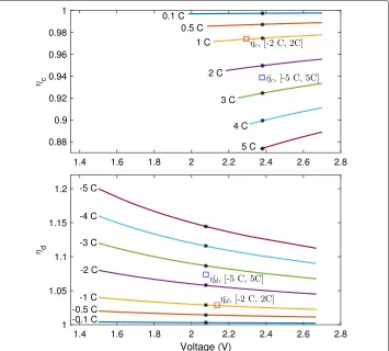
To illustrate the efficiency functions and the effect of the approximations, the charging and discharging efficiencies of an LTO cell is shown in Fig.4, with solid lines represent-ing Eqs.7and8, asterisks representing the efficiencies when calculated using a constant approximation of the charging voltage asVnom,c andVnom,d, and squares representing constant efficiency approximations.
Fig. 4The charging and discharging efficiencies of an LTO cell withRic=Rid=0.002m. Each solid line
represents the efficiency calculated using Eqs.7or8at the labeled charging/discharging C-rate. Each asterisk represents the approximation whereV=Vnom,cfor charging andVnom,dfor discharging. The constant
Operating Range
The operating range (OR) is an important parameter to consider when calculating the approximations to different curves. We define the OR as the range of currents that we expect to be applied to the battery. The intuition is that we should match the parameters of the modelled battery to reflect the actual operation of the battery, rather than calibrating the model to be as accurate as possible over the full OR capabilities of the battery. Indeed, some applications do not use the full OR. When the OR is narrow, we can expect a lower modelling error.
In Figs.2,3, and4, the approximations to the corresponding functions were computed over the full operating range ([-5 C, 5 C] for the LTO cell) unless otherwise noted. In this paper, we compute the constant approximations to be equal to the average value of their corresponding curve over the OR, and choose linear approximations that minimize the least-squared error to the curve over the OR. For example, Fig.4shows the constant approximation for charging efficiency(ηc)¯ and discharging efficiency(ηd)¯ for the full OR of [-5 C, 5 C] as well as for a narrower OR of [-2 C, 2 C];ηc¯ is higher for the narrower OR because the efficiency is higher at lower C-rates.
Models
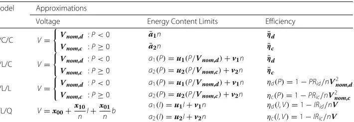
We have developed notation to refer to each of the four models that we describe next, based on how the voltage, energy limits, and efficiencies are approximated. Similar to Kendall’s notation for queues (Kendall1953), each component of the model is described by a letter with slashes in between, i.e., Voltage function/Energy limit/Efficiency (V/E/η) notation. A letter ‘Q’ means that that calculation uses a quadratic approximation, such as the voltage function in the PI model; ‘L’ represents a linear approximation, and ‘C’ a constant approximation5.
The four analytic models are summarized in Table2, and we describe them below. Out of the four models, three approximate the voltage using two constantsVnom,candVnom,d. For these three models, we can write their formulation in terms of power by replacing
I(k) > 0 byP(k)/Vnom,candI(k) < 0 byP(k)/Vnom,d in the PI model and can remove Eqs.9and10completely.
C/C/C
This model is exactly the benchmark summarized in Eqs.1–4, and we henceforth refer to it as the C/C/C model. It uses constant approximations for efficiencies and energy
Table 2Summary of Analytical Models Model Approximations
Voltage Energy Content Limits Efficiency
C/C/C V=
Vnom,d :P<0 Vnom,c :P≥0
¯ a1n
¯ a2n
¯
ηd ¯
ηc
C/L/C V=
Vnom,d :P<0 Vnom,c :P≥0
a1(P)=u1(P/Vnom,d)+v1n
a2(P)=u2(P/Vnom,c)+v2n ¯
ηd ¯
ηc
C/L/L V=
Vnom,d :P<0
Vnom,c :P≥0
a1(P)=u1(P/Vnom,d)+v1n
a2(P)=u2(P/Vnom,c)+v2n
ηd(P)=1−PRid/nV2nom,d
ηc(P)=1−PRic/nV2nom,c
L/L/Q V=x00+ x10
n I+
x01
n b
a1(I)=u1I+v1n
a2(I)=u2I+v2n
ηd(I,V)=1−IRid/nV
ηc(I,V)=1−IRic/nV
limits, and a constant approximation of the voltage. It is linear (see the discussion in “The Benchmark Model” section) and all the equations can be written in terms ofb(k)and
P(k)only. It has low energy estimation errors when the OR is narrow (Kazhamiaka et al.2016), and hence it is important to calibrate it with respect to the OR. Treating the benchmark model as a derivative of the PI model makes the calibration procedure (see “Methodology” section) clear, as it utilizes the available spec data, and thereby improves model accuracy. For example, the charging efficiency calculated for an LTO battery with an OR of [-5 C, 5 C] is 0.94, and is increases to≈0.975 for an OR of [-2 C, 2 C]; for a Lithium-Ferrous-Phosphate (LiFePO4) battery (A123 Systems2009), the efficiency for an OR of [-2 C, 2 C] is calculated to be≈0.985.
C/L/C
This model uses constant approximations of the charging and discharging voltage as well as charging and discharging efficiencies, and uses a linear approximation to the energy content limits. Similarly to the C/C/C model, all the equations can be written in terms of
b(k)andP(k)only. Notably, it has the same complexity as the C/C/C model (linear), while offering a better approximation to the energy limits.
C/L/C:
b(k)=b(k−1)+E(k) (19)
E(k)=
¯
ηcP(k)Tu :P(k)≥0 ¯
ηdP(k)Tu :P(k) <0
(20)
nαdVnom,d≤P(k)≤nαcVnom,c (21)
u1 P(k) Vnom,d +
v1n≤b(k)≤u2 P(k) Vnom,c +
v2n (22)
C/L/L
This model uses constant voltage approximations, the same efficiency formula as the PI model, and linear energy content limits. The constant voltage approximation makes the efficiency function linear. Note that in the formulation, we have excluded an explicitI(k)
term since, due to the constant voltage approximations, the current is estimated as either
P(k)/Vnom,corP(k)/Vnom,d. Hence, all the equations can be written in terms ofb(k)and P(k). Altogether, this model is quadratic inP(k).
C/L/L:
b(k)=b(k−1)+E(k) (23)
E(k)=
ηc(P(k))P(k)Tu :P(k)≥0 ηd(P(k))P(k)Tu :P(k) <0
(24)
ηc(P(k))=1− P(k)Ric
nV2 nom,c
(25)
ηd(P(k))=1− P(k)Rid
nVnom,d2 (26)
nαdVnom,d≤P(k)≤nαcVnom,c (27)
u1 P(k) Vnom,d +
v1n≤b(k)≤u2 P(k) Vnom,c +
L/L/Q
This is the most complex of our explicit models. It combines a linear bivariate voltage function, the same quadratic efficiency formula used in the PI model, and a linear approx-imation for the energy limits. The formulation resembles that of the PI model with the voltage and energy limits replaced by explicit functions. The model is
L/L/Q:
b(k)=b(k−1)+E(k) (29)
E(k)=
ηc(P(k))P(k)Tu :P(k)≥0 ηd(P(k))P(k)Tu :P(k) <0
(30)
ηc(I(k))=1− I(k)Ric
nV(k) (31)
ηd(I(k))=1−I(k)Rid
nV(k) (32)
V(k)=x00+ x10
n I(k)+ x01
n b(k) (33)
I(k)= P(k)
V(k) (34)
nαd≤I(k)≤nαc (35)
u1I(k)+v1n≤b(k)≤u2I(k)+v2n (36)
Note that all the equations can be written in terms ofb(k),I(k)andP(k)and the model is non-linear in bothI(k)andP(k). Hence, this model is much more complex and difficult to use.
Evaluation
In our evaluation, for each of the analytic models discussed in the “Models” section, we quantify the loss of accuracy in the energy content estimate with respect to the PI model. We take this approach because measuring the energy content of a battery directly is very difficult. Hence, we use the PI model to estimate the energy content of the battery, since prior work has found it to accurately model battery dynamics.
More precisely, to evaluate our models, we use LTO (Leclanché2014) and Lithium-Ferrous-Phosphate (LiFePO4) (A123 Systems 2009) battery measurements collected while running charge/discharge cycling experiments on these batteries at different C-rates with 2-3 cycles per C-rate, and use the PI model to calculate the energy content of these batteries over the course of the experiment. We then recreate these experiments using simulations of each one of our tractable models, assuming the same applied power that was used in our experiments. We then compare the energy content in the battery over time as simulated by each of our models to the energy content calculated by simulating the battery using the PI model.
Constant-current cycles
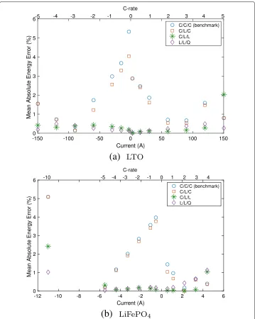
(a)
(b)
Fig. 5Mean absolute energy error for LTO cell (a) and LiFePO4 cell (b) for constant-current cycles at different C-rates (top scale)/Amperes (bottom scale)
mimics their order in terms of complexity. The relative differences in accuracy between the models can be used to understand how much error each approximation contributes. For example, having a linear voltage function (L/L/Q) offers little improvement in accu-racy over using two constants (C/L/L) for all but the most extreme C-rates. C/C/C and C/L/C have low errors around 2-3 C for LTO for both charging and discharging, and at 5C discharging and 2 C charging for LiFePO4 because the constant efficiency approximation happens to be close to the PI model’s efficiency at these currents, as shown for an LTO cell in Fig.4.
appears to be the case in the 5 C charging test for the LTO battery, where the errors of the C/C/C and C/L/C models are lower than the C/L/L model error.
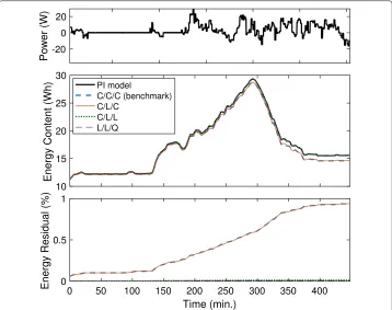
Varying charge/discharge profile
To evaluate the accuracy of the models in a realistic setting, we conducted an experiment which mimics the charge/discharge pattern if an LTO battery were installed in a building with photovoltaic (PV) panels, and used as a buffer to store excess PV solar generation and provide power to the building when PV was not enough. We then simulated this system using our analytic models which were calibrated with an OR of [-2 C, 2 C], and with the PI model to use as our benchmark. Figure6shows the power profile used in our experiment, the resulting energy content evolution over an 8-hour period, as well as the residual with respect to the PI model’s energy content estimate. This experiment highlights the effect of the efficiency and voltage function approximations, since the battery did not approach any energy content limits over the course of the test. The residual for all the models stays below 1% of the total energy capacity of the LTO battery, with the residual of C/L/L and L/L/Q models well below 0.1%.
From these experiments alone, it is unclear if 1% or 0.1% residuals are low enough for us to get useful results when these models are used for energy system analysis. Likewise, the MAEE is not easy to relate to the impact of these errors on the actual application of these models. For this reason, we next compare these models in terms of their performance in two case studies.
Applications
We performed case studies that compare the accuracy of our models with respect to the PI model for relevant metrics in two battery applications: a solar farm firming application, and grid regulation services. The purpose of these case studies is to exhibit the effects of the choice of battery model on the conclusions that are made. Both case studies are performed via simulations and will be described next.
To obtain results with the proper operating range (OR), which differs for a given appli-cation and battery size6. We run each simulation twice. First, we calibrate the model with the maximum OR of the battery, i.e., [αd,αc], and simulate the application. We then observe the OR that was actually used in the simulation, re-calibrate the model, and run the simulation a second time. We report the results from the second simulation.7
Solar farm firming
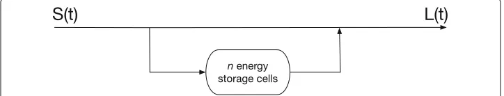
We consider a small (100 kW) solar farm participating in an electricity market with hourly power commitments and penalties for failing to adhere to the commitment. Figure 7 shows the basic structure of the system, whereS(t)is the incoming solar power which we model using measured data. The loadL(t)represents the hourly power commitment that is made by the operator. We assume that the operator always commits to providing the average hourly solar production, and a battery is used to firm the intra-hourly fluctuations in PV production.8
An important metric in this application is the amount of energy that was needed from the battery but not delivered, i.e., when not enough PV is being generated to meet the power commitment and the operator needs to discharge the battery but is unable to because the battery does not have enough energy or the required power is too high for the battery to provide. We call this theunmet loadon the battery. Choosing a battery size to meet an unmet load target is a classic optimization problem. To see the difference that the choice of battery model will make on the conclusions of this study, we calculate the unmet load by simulating the system with a solar measurement trace for 100 days across a range of battery sizes.
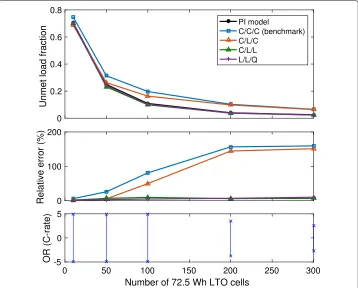
We present results with the model calibrated for the LTO battery chemistry, and remark that we obtained similar results for the LiFePO4chemistry. Figure8shows the unmet load calculated for different battery sizes using the PI model as well as the four analytic models, and the OR used to calibrate model parameters for each battery size. The relative error is very low for the L/L/Q and C/L/L models, and very high for C/C/C and C/L/C models.
The C/L/C model has a low error for 10 and 50 cell batteries, and high error for larger sizes; this is due to the OR and its effect on the different parameters. For smaller battery sizes, the OR is maxed out at [-5 C, 5 C], although the actual currents are much more
Fig. 8Unmet load for different battery sizes, computed using five different models. Relative error is with respect to the PI Model, and the effective OR calculated by the PI model is shown in the bottom-most figure
uniformly distributed across the OR with a small (10 - 50 cell) battery compared to the 100-cell battery where the 5 C is a rare occurrence. The OR gradually narrows as the number of cells increases to 300. For a large OR, it is crucial to model the energy limits as a function of the current, which is why the C/L/C model outperforms the C/C/C model. For narrower OR, the efficiency estimate becomes a more important factor as demonstrated by the high accuracy of L/L/Q and C/L/L models and the similar (poor) accuracy of C/L/C and C/C/C models.
The conclusions of this study can vary greatly depending on the choice of battery model. For example, if the purpose of the study is to determine the smallest battery size that is sufficient to achieve an unmet load target of 40%, all models suggest a similar size. However, for a more realistic 10% target, the size suggested by the C/C/C and C/L/C models is over 2x larger than the size suggested by the C/L/L and L/L/Q models. The main message is that neither of the linear models works well for this application, and a more complex model such as C/L/L is needed to get accurate results.
Regulation
contract. In this case study, we model an LTO battery and fix the energy content at the start of the contract to 50% of the battery’s maximum capacity.
We presents the results for down-regulation, where the battery is discharged. Figure9 shows the power that the battery can consistently provide for various contract durations. We also compute the relative error with respect to the results obtained using the PI model. The C/C/C model has very poor accuracy for all contract lengths, which can be explained by noting that the energy limit is the most important parameter for this application. The L/L/Q model has slightly larger errors (up to 5%) than the C/L/C and C/L/L models, which is not an intuitive result and is an important observation; since we are dealing with approximations of multiple components of the PI model, there is room for errors introduced by these components to cancel each other out. Indeed, the improved voltage estimate of the L/L/Q model in turn leads to an accurate current estimate, which is then used to calculate efficiency and energy limits, while the constant voltage approximation in C/L/L and C/L/C models leads to a poor current estimate which actually ends up partially negating the errors in the energy limit approximation. The main message here is that a linear model (C/L/C) is accurate enough for this application.
To highlight the effect of the OR on the accuracy of the models, we have calculated the results for the regulation application with a full OR ([-5 C, 5 C]) for all contract lengths. Figure10shows the power commitment suggested by the C/C/C, C/L/C, and C/L/L mod-els with a full OR, compared to the same modmod-els calibrated with the actual OR of the application for each contract length. Every model has worse accuracy when calibrated for the full OR. Note that the L/L/Q model is not shown because its accuracy is almost
Fig. 10 Computed vs. full OR calibration for the regulation application
unchanged when calibrating for a narrower OR; this is an intuitive result, as the L/L/Q model uses better approximations which are not as sensitive to the OR.
Discussion and Limitations
Our extensive experimentation with different models and calibration methods has given us insight into how to choose and calibrate a battery model for energy system analysis, in particular for system control and sizing optimization studies. Below, we outline four considerations in selecting a model.
1. What is the size of the optimization problem? For small problems that could be solved by non-linear optimization methods in a reasonable time frame, the L/L/Q and C/L/Q models could be used. Large problems require efficient methods such as linear programming, which require a linear model. In this case, we suggest using the C/L/C model, since it is more accurate than the commonly used C/C/C model, with no added complexity.
2. What battery chemistry is being modelled? Some chemistries, such as LiFePO4, have “flat” voltage profiles which can be approximated well as a constant voltage. Cells with very low internal impedance have high efficiency values (close to 1) which could be closely approximated using a constant. The area under the voltage curve for different C-rates on a voltage vs. charge graph (commonly found in a spec sheet) can hint at the shape of the energy limit function10. This information can help guide the choice of battery model.
4. What is the operating range of the application? If it is known a priori, it should be used to calculate the parameters of the battery. If it is unknown, the analysis should first be conducted with the model calibrated using the maximum OR that the battery allows, keeping track of the OR that is actually used by the battery in the analysis. Then, the analysis should be re-run with parameters computed for the OR observed in the first analysis. This can be repeated until the calibrated OR matches the observed OR; in our experience, we noticed that there was little benefit in going beyond one or two iterations of this method.
Our work has two main limitations. The first is that we have only evaluated our model on two Lithium-ion battery chemistries; we defer the testing of a broader range of electro-chemical storage technologies to future work. Finally, there are limitations to the PI model that are inherited by the tractable models we have derived: it does not model the effects of temperature on the battery, and does not take the battery state of health and degradation into account.
Conclusion
We propose three novel, analytical, and easily-calibrated battery models which are derived from the PI model: the C/L/C, C/L/L, and L/L/Q models. These models were obtained by using a methodology that involves measuring the effect of different degrees of approximations to complex and non-analytic PI model components, and selecting the models with a desirable trade-off between accuracy and complexity. In our evaluation, we compare the accuracy of the derived models in three settings: constant-current cycling, a real-world charge/discharge profile, and two energy system case studies. In particular, we show that the C/L/C model is more accurate and just as tractable as the benchmark model for optimization studies. We also show that the choice of model can significantly affect the conclusions of model-based energy system studies and that sometimes a non linear model (C/L/L) is necessary. Finally, we show that the operating range of the battery is a crucial parameter for obtaining accurate results with simplified models.
Endnotes
1PI stands for “Power-based Integrated”, because it uses power as input and integrates
the BMS and cell models into a single model.
2If the spec sheet provides only one value for internal impedance, then we use that
value for bothRicandRid.
3To scale these equations to more than one cell, we divideI(k)andb(k)bynwherever
they appear.
4We use MATLAB’sfitfunction to compute the linear approximation.
5Technically, the voltage approximation given in Eq.13corresponds to two constants
instead of one.
6The effect of the battery size on the OR, which is given in terms of C-rate, can be
explained concisely via example: an application may require a current of 100 Amps, which equates to 1 C for a particular battery, but only 0.5 C when the battery’s size is doubled
7One could continue re-running simulations using the OR observed in the previous
8A comprehensive study of this system can be found in Ghiassi-Farrokhfal et al. (2015). 9A comprehensive study of this application can be found in Fooladivanda et al. (2016) 10The area under a discharging voltage vs. charge curve is equal to the energy
discharged from the battery at the given C-rate.
Abbreviations
BMS: Battery management system; LP: Linear program; LTO: Lithium-titanate; LiFePO4: Lithium-ferrous-phosphate; MAEE: Mean absolute energy error; OR: Operating range; PI: Power-based integrated battery model; PV: Photovoltaic
Acknowledgements
We acknowledge Prof. Karl-Heinz Pettinger and the technicians at the Ruhstorf Technology Center for Energy for helping us run the experiments that contributed to the evaluation of our models.
Funding
None to declare.
Availability of data and materials
The data sets used to drive the evaluation of the models are available from the corresponding author on reasonable request.
Authors’ contributions
All of the authors worked together to conceive the ideas summarized in this paper, and to write and review the paper. The implementation of the models in MATLAB, their evaluation, and application testing was done by FK. All authors read and approved the final manuscript.
Competing interests
The authors declare that they have no competing interests.
Publisher’s Note
Springer Nature remains neutral with regard to jurisdictional claims in published maps and institutional affiliations.
Received: 6 February 2019 Accepted: 12 April 2019
References
A123 Systems (2009) High Power Lithium Ion APR18650M1A. A123 Systems. LiFePO4 cell specifications.https://blizzard. cs.uwaterloo.ca/iss4e/wp-content/uploads/2019/04/A123-APR18650M1A.pdf
Atia R, Yamada N (2016) Sizing and analysis of renewable energy and battery systems in residential microgrids. IEEE Trans Smart Grid 7(3):1204–1213
Chen M, Rincon-Mora GA (2006) Accurate electrical battery model capable of predicting runtime and iv performance. IEEE Trans Energy Convers 21(2):504–511
Chen S, Gooi HB, Wang M (2012) Sizing of energy storage for microgrids. IEEE Trans Smart Grid 3(1):142–151 Einhorn M, Conte FV, Kral C, Fleig J (2013) Comparison, selection, and parameterization of electrical battery models for
automotive applications. IEEE Trans Power Electron 28(3):1429–1437
Fooladivanda D, Rosenberg C, Garg S (2016) Energy storage and regulation: an analysis. IEEE Trans Smart Grid 7(4):1813–1823
Gearhart JL, Adair KL, Detry RJ, Durfee JD, Jones KA, Martin N (2013) Comparison of open-source linear programming solvers. Tech. Rep. SAND2013-8847
Ghiassi-Farrokhfal Y, Kazhamiaka F, Rosenberg C, Keshav S (2015) Optimal design of solar pv farms with storage. IEEE Trans Sustain Energy 6(4):1586–1593
Ghiassi-Farrokhfal Y, Rosenberg C, Keshav S, Adjaho M-B (2016) Joint optimal design and operation of hybrid energy storage systems. IEEE Journal Sel Areas Commun 34(3):639–650
Hassan AS, Cipcigan L, Jenkins N (2017) Optimal battery storage operation for pv systems with tariff incentives. Appl Energy 203:422–441
He H, Xiong R, Zhang X, Sun F, Fan J (2011) State-of-charge estimation of the lithium-ion battery using an adaptive extended kalman filter based on an improved thevenin model. IEEE Trans Veh Technol 60(4):1461–1469 Hentunen A, Lehmuspelto T, Suomela J (2014) Time-domain parameter extraction method for thévenin-equivalent
circuit battery models. IEEE Trans Energy Convers 29(3):558–566
Hu X, Li S, Peng H (2012) A comparative study of equivalent circuit models for li-ion batteries. J Power Sources 198:359–367 Jackey R, Saginaw M, Sanghvi P, Gazzarri J, Huria T, Ceraolo M (2013) Battery model parameter estimation using a layered
technique: an example using a lithium iron phosphate cell. Technical report. SAE Technical Paper
Kazhamiaka F, Keshav S, Rosenberg C, Pettinger K-H (2018) Simple spec-based modelling of lithium-ion batteries. IEEE Trans Energy Convers 33:1757–1765
Kazhamiaka F, Rosenberg C, Keshav S, Pettinger K-H (2016) Li-ion storage models for energy system optimization: the accuracy-tractability tradeoff. In: Proceedings of the Seventh International Conference on Future Energy Systems. ACM. p 17
Kendall DG (1953) Stochastic processes occurring in the theory of queues and their analysis by the method of the imbedded markov chain. Ann Math Stat:338–354
Klein R, Chaturvedi NA, Christensen J, Ahmed J, Findeisen R, Kojic A (2013) Electrochemical model based observer design for a lithium-ion battery. IEEE Trans Control Syst Technol 21(2):289–301
Leclanché (2014) LecCell 30Ah High Energy. Leclanché. Lithium-Titanate cell specifications.https://blizzard.cs.uwaterloo. ca/iss4e/wp-content/uploads/2019/04/leccell-30ah-high-energy.pdf
Mehrabankhomartash M, Rayati M, Sheikhi A, Ranjbar AM (2017) Practical battery size optimization of a pv system by considering individual customer damage function. Renew Sust Energ Rev 67:36–50
Scrosati B, Hassoun J, Sun Y-K (2011) Lithium-ion batteries. a look into the future. Energy Environ Sci 4(9):3287–3295 Tanim TR, Rahn CD, Wang C-Y (2015) A temperature dependent, single particle, lithium ion cell model including
electrolyte diffusion. J Dyn Syst Meas Control 137(1):011005
Zou C, Manzie C, Neši´c D (2016) A framework for simplification of pde-based lithium-ion battery models. IEEE Trans Control Syst Technol 24(5):1594–1609
Submit your manuscript to a
journal and benefi t from:
7Convenient online submission
7Rigorous peer review
7Immediate publication on acceptance
7Open access: articles freely available online
7High visibility within the fi eld
7Retaining the copyright to your article