Reliability Design for Large Scale Data
Warehouses
Kai Du1, Zhengbing Hu2, Huaimin Wang1, Yingwen Chen1, Shuqiang Yang1, Zhijian Yuan1 1School of Computer Science, National University of Defense Technology, Changsha, China
2Department of Information Techonolgy, Huazhong Normal University, Wuhan, China
Email: [email protected]
Abstract—Data reliability has been drawn much concern in
large-scale data warehouses with 1PB or more data. It highly depends on many inter-dependent system parameters, such as the replica placement policies, number of nodes and so on. Previous work has roughly and separately discussed the individual impacts of these parameters, and seldom provided their optimal values, nor mentioned their optimal combination. In this paper, we present a new object-based-repairing Markov model. Based on analyzing this model in three popular replica placement policies, we figure out the individual optimal values of these parameters at first, and then work out their optimal combination by GA. Compared with the existing models, our model is easier to solve while reaching more integrative and practical conclusions. These conclusions can effectively instruct the designers to build more reliable large-scale data warehouses.
Index Terms—data reliability, reliability model, large-scale
data warehouse
I. INTRODUCTION
Many applications depending on large scale storage have emerged in many domains, such as scientific experiments, telecom companies, huge Internet search engine companies, and so on. For example, the National Energy Research Scientific Computing Center database encompasses 2.8 petabytes (PB, 1015 bytes) of information; AT&T data warehouse stores 323 terabytes of calling records [1]. These systems are often built on clusters of storage nodes, each of which is equipped with CPU, memory and disks. Another trend in large scale storage systems is to store more and more WORM (Write Once Read Many) data [7]. These large storage systems or large-scale data warehouse, built with vast storage components, trend to have high failure probability [8, 19] and long recovery time. Therefore, it is a significant challenge to build a high reliable large data warehouse.
Many solutions have been proposed for data reliability. Replication is a widely used mechanism to protect permanent data loss while replica placement will significantly impact data reliability. Aiming at different objectives, several replica placement policies have been proposed and deployed in real-world systems, such as RANDOM in GFS [3], PTN in RAID [16], Q-rot in [9].
Q. Lian and Chen [10, 11] have analyzed how the system parameters, such as system capacity, object size, disk and switch bandwidth, could affect the system’s reliability. However, they only discussed the rough trend about their impact but did not illustrate the accurate optimal values of these parameters. In addition, the co-impact of these parameters was not discussed. Furthermore, aiming to get the accurate reliability value, some models are so complex that it is difficult to figure out the optimal value of each parameter.
The limitations above bring about the motivation of this paper: to design a reliable system with the optimal system parameters. Compared with previous work, our approach makes a significant contribution in two aspects. Firstly, we present a new object-based Markov model to quantify the impact of key system parameters on the system reliability in three replica placement policies. These key system parameters can be the total number of nodes, total number of objects, switch bandwidth, disk bandwidth and so on. Compared with previous complex models, this object-based compact model not only turns to be easier to solve because of its smaller state transition matrix, but also leads to more integrative and practical results. Secondly, we propose a two-step analyzing process. The first is to find out the relatively accurate optimal value of a system parameter by independently analyzing its impact on the system reliability when other system parameters are fixed. The second is to figure out the optimal combination of these parameters by analyzing their integrated and complex impacts on the system reliability while all of them are tuned. The analysis results show that the optimal values do exist and have simple formulas.
II. PLACEMENT POLICIES AND DATA RELIABILITY
DEFINITION
How to place objects’ replicas to the storage nodes dramatically influences the system reliability. This section will introduce three classic placement policies and their data reliability. The reason of analyzing these three policies is that they are well-designed for reliability. A. Three Replica Placement Policies and Repairing Strategy
Before introducing the policies, we assume n unique objects are stored on N storage nodes and every object has K replicas. A replica placement policy is responsible for designating the mapping relationship between replica and storage node. Generally, two same replicas will not be placed on a same node.
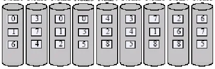
The first policy is RANDOM, which randomly assigns a replica to a machine. The systems, such as GFS [3], FARSITE [12], and RIO [13] adopt this policy. Figure 1 shows the case that nine objects (each with 3 replicas) are randomly placed on nine nodes. With RANDOM placement, once a node fails, the replicas on the failure node can be found on many other nodes, and thus these nodes can participate in repairing in parallel. This significantly improves the repairing rate.
The second one is PTN [14] which manually partitions the objects into sets and then mirror each set across K nodes. This policy has been adopted in RAID [16] and Coda [15]. A classic PTN is illustrated in Figure 2. With PTN placement, if a node fails, the replicas on the failure node can only be repaired by the other K-1 nodes, that is, its parallel repairing degree is far lower than RANDOM. However, the advantage is that its object failure probability is lower than that of RANDOM.
The third one is Q-rot [9], which partitions all the nodes into N/K sites and each site is the replica of others. It subtly places replicas on each site to achieve the objective that the number of intersecting replicas of any two nodes is 1. This maximizes the repairing rate and reaches the optimal rate in RANDOM. Figure 3 presents an example of 9 objects on 9 nodes (3 sites). With Q-rot placement, when a node fails, the replicas on the failure node can be repaired from many nodes (at most (N-1)/2) in parallel like RANDOM. The advantage is that it has the same low failure probability as PTN while achieves the same or better repairing rate compared with RANDOM.
For each replica placement policy, there are two primary maintenance operations: object repair and object rebalance. The former one is the process of regenerating lost replicas after node failures; while the latter one is the process of migrating data to the new replacement nodes.
Figure 1. RANDOM placement of 3 replicas. At most 3 nodes participate as source nodes in repairing one node failure.
Figure 2. PTN placement of 3 replicas. At most 2 nodes participate as source nodes in repairing for one node failure.
Figure 3. Q-rot placement of 3 replicas. Always 3 nodes participate as source nodes in repairing for one node failure.
B. Concept of Data Reliability
Data reliability refers to how long a system sustains before the first object is lost. In this paper, we use Mean Time To Data Loss (MTTDL) to denote the data reliability. In a storage system, an object’s reliability is observably different from the system reliability since one node always stores many replicas. Consequently, we quantify the system reliability by measuring the object’s reliability together with the objects’ dependence.
Object Reliability MTTDLO
Object Reliability MTTDLOis defined as the mean time when all the replicas of an object are lost. The object’s mean time to loss is influenced by two factors: object failure probability and repairing rate. The former is determined by disk failure probability and object placement policy, and the latter is measured by the object average size and the parallel repairing bandwidth. System Reliability MTTDLS
Assuming the number of independent objects is ni, we define the system reliability MTTDLS, which denotes the mean time to any object data loss, as follows:
MTTDLS = MTTDLO / ni . (1) If every replica of two objects is on the same node, in other words, the two objects have the same placement, these two objects are called dependent; otherwise they are independent because one’s failure will not affect the other. With this weaker independence definition we arrive at a strict MTTDLS. The ni of the three placements is in Table I. K
N
C denotes the total number of combinations of picking K nodes from N nodes to place K replicas.
TABLE I. THREE REPLICA PLACEMENT’S NI FORMULA
RANDOM Q-rot PTN
ni min( m*⎡⎢N K/ ⎤⎥ , K
N C )
min(m*⎡⎢N K/ ⎤⎥ ,⎡⎢N K/ ⎤⎥2)
III. SYSTEM RELIABILITY ANALYSIS
From Section II, we can conclude that the data reliability is related with three factors: an object’s failure probability, repairing rate and inter-dependence. In this section, after defining the system parameters, we firstly discuss the former two factors and then use a Markov model to describe the object fault and repairing process. A. System Parameters
Table II lists the system parameters used in our later analysis. The former four parameters not only take remarkably impacts on the system failure probability and the repairing rate, but also have correlated optimal values to calculate MTTDLS. Therefore, we will focus on their impacts on MTTDLS. The rest parameters are considered as constants because their impacts are simple. For example, the smaller the system data capacity S, the larger the replica degree K, or the smaller the node failure rate λ, the larger the system reliability. So in the rest of this paper, the value of K , λ, and S will be set as the default value in Table II.
TABLE II. SYSTEM PARAMETERS
Parameter Signification Default
N Number of total nodes variable
m Average number of
objects stored in a node variable
B Switch bandwidth variable
b Node IO bandwidth variable
q Fraction of B and b
allocated for object repair; (1-q) for object rebalance
90%
K Number of replicas
per object 3
λ Failure rate of a node 1/3 (1/year)
S Amount of data 1PB
n Number of total
unique objects N*m/K
s Size of an object S/(N*m)
ni Number of
independent objects
In Table I
nf Average number of
failure nodes in one day ⎡⎢Nλ/ 365⎤⎥ nr Number of objects to
be repaired in parallel m n* f B. Fragility Analysis: Failure Probability
In many applications, one request often accesses multiple objects, such as database applications and compiling projects with multiple code files. Thus, we need to analyze the system failure probability (ab. FP) by evaluating FP of multiple objects.
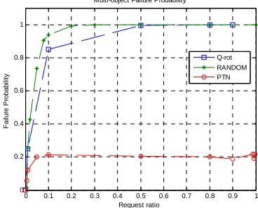
Multi-object’s FP can’t be figured out directly because the number of objects accessed by a request is not fixed. So we get the multi-object’s FP by simulations. In Figure 4, the x-axis is the request ratio (the ratio of the requested objects number to the total object number in one request); the y-axis is the multi-object’s FP; the object failure
probability is 0.1. It indicates that PTN has the lowest and const FP of 0.2 while RANDOM and Q-rot are worse. So PTN is the most robust in these three replica placement strategies in availability. Another set of results of simulations are: 1) the smaller n, the lower the FP in RANDOM and Q-rot; 2) the smaller N, the lower the FP in PTN; 3) the smaller N and n, the lower the FP in RANDOM and Q-rot.
0 0.1 0.2 0.3 0.4 0.5 0.6 0.7 0.8 0.9 1
0 0.2 0.4 0.6 0.8 1
Request ratio
Fa
ilu
re
P
ro
b
a
b
ilit
y
Multi-object Failure Probability
Q-rot RANDOM PTN
Figure 4. Multi-object’s failure probability
C. Recoverability Analysis: Repairing Rate
From Section II.A, we know although the minimum failure unit is referred as a storage node, in the repairing process, the minimum repair unit is an object. In the repairing process, many objects may be repaired in parallel with the same priority. Consequently, the repairing time of an object equals to its size divided by the average bandwidth (Because the cost of maintaining updated data consistency in the WORM data repairing is zero). The average repairing bandwidth (rpb) is determined by four factors: the total repairing bandwidth of participant source nodes, bandwidth of destination nodes, bandwidth of switch, and the number of objects to be simultaneously repaired. It is computed as: rpb = min (source nodes’ bandwidth, destination nodes’ bandwidth, switch bandwidth) / (number of objects to be repaired), because the minimum of the three is the real repair bandwidth.
The number of objects to be simultaneously repaired nr, is not a constant, but we can estimate its average value by multiplying the number of failure nodes in one day nf with the number of objects in a node m, that is:
= * = * / 365
r f
n m n m ⎡⎢Nλ ⎤⎥ (2)
As we know, three replica placement policies leading to different repairing bandwidth can be analyzed respectively as follows. In PTN, the maximum bandwidth of the participant source nodes is (K-1)bq, that of the destination nodes is (N- nf)bq. Generally speaking, B/b>> K-1, (N- nf)>> K-1, therefore, the object’s repairing bandwidth is:
min(( -1) , ( - ) , )f ( -1) PTN
r r
K bq N n bq Bq K bq
rpb
n n
= = (3)
-( - )
= min( f , , )
Q rot RANDOM
r r
bq N n Bq
rpb rpb bq
n n
= (4)
As discussed in [9], Q-rot uses almost all healthy nodes to participate as source nodes in object repairing, if the number of failure nodes is large enough. With this conclusion, we use (N-nf) to denote the number of source nodes. In (4), b and B is the duplex bandwidth.
In RANDOM, although rpbRANDOM has the same formula as Q-rot, it is only a statistical value. In Q-rot, rpb is a determination value that can be calculated through a specified placement.
Another repairing factor to be discussed is the object rebalance rate. Just like the object repairing rate, only the rebalance bandwidth of an object requires to be considered. The rebalance bandwidth of all the three placement policies has the similar formula as follows:
- = min( / , (1 ))
PTN Q rot RANDOM
rbb =rbb =rbb b m b −q
D. Markov Reliability Model
With the predication of the analysis results in Section III.B and III.C, N or n contradictorily affect both the system fragility and recoverability. Analyzing such synthetical effects places stringent demands on a new reliability model.
In Section II.B, we have defined the system reliability quantified by calculating the object’s reliability. Consequently, we build a continuous-time Markov process shown in Figure 5. This object-based model depicts the failure and the repairing process of replicas.
Figure 5. Object-based data maintenance process
A state in the process is defined with (k, i), where k denotes the number of normal replicas of the observed object on the initial node, i presents the number of repaired replicas of the observed object which are temporarily stored on some nodes and wait to be rebalanced to the new replaced node. The initial state (K, 0) means K replicas (defined in Table II) are all on initial nodes. The only absorbing state (0, 0) means all replicas of the observed object have been lost. MTTDLO is the mean time from the initial state (K, 0) to (0, 0).
To quantify MTTDLO, the transition rates between all states need being described. λ is a replica’s failure rate in Table II. µ is the repairing rate of an object replica, and ν
is the rebalance rate of a replica. They can be calculated as the following according to Section III.C and Table II: µ = rpb/s and ν = rbb/s.
After all the transition rates are figured out, MTTDLO is calculated on the transition matrix with the procedure in [17]. MTTDLO = f(µ, ν, λ,K) is such a complex function that it is not expressed here. After analyzing MTTDLO, we find out that (c is a constant):
MTTDLO ≈ c*µ2 (5) Compared to the model proposed in [11], our model is simpler because it ignores the nodes’ repairing, which is unrelated to the current observed object. The model in [11] emphasizes on the repair of nodes and objects, whereas ours focuses on the repair of objects assuming an average number of failure nodes. Thus the number of states in our model is O(K2) while [11] is O(NK). Since N>>K and N may trend to be larger than 1000 in a large-scale system, it is a challenging work to solve this huge matrix. In our model, it is not so accurate as [11] since it ignores the number of current failure nodes. However, in our concerned application scenarios we pay much more attention to the optimal system parameters rather than the accurate reliability value itself.
IV. OPTIMAL SYSTEM PARAMETERS FOR RELIABILITY
This section will figure out the optimal values of the four parameters, m, B, b and N, by illustrating their individual impact on MTTLS (Just as interpreted in Section III.A, the impacts of other parameters will not be analyzed.). In order to simplify analyzing MTTLS, we need to simplify the parameters in MTTDLO = f(µ, ν, λ ,K) as follows: (The approximation conditions in the two formulas are N−nf ≈ N and⎢⎡Nλ/ 365⎤⎥≈ Nλ/ 365.):
-min( / , (1 )) =
PTN Q rot RANDOM
b m b q
S Nm
ν =ν =ν −
(6)
-min( ( - ), )
min( , )
=
min( ( - ), )
min( , ) 365
/ 365 min( , , )
365
f
r Q rot RANDOM
f
bq N n Bq bq n
S Nm bq N n Bq
bq Nbq Bq Nmbq
mN
S S
Nm
µ µ
λ
λ λ
=
≈ ≈
(7)
( -1)
365( 1)
= f
PTN
K bq
mn K bq
S S
Nm
µ
λ −
≈ (8)
Therefore we can transform MTTLS into the following according to (1), (5) and the above (c’ and c’’ are both constant):
2 2
2
-'*[min( , , )]
* 365
/ /
min( * , )
S Q rot i
Nbq Bq Nmbq c
c
n N K N K
MTTL
m
µ λ λ
≈ =
⎡ ⎤ ⎡ ⎤
⎢ ⎥ ⎢ ⎥
(9)
2 2
-'*[min( , , )]
* 365
/
min( * , K)
N S RANDOM
i
Nbq Bq Nmbq c
c
n N K C
MTTL
m
µ λ λ
≈ =
⎡ ⎤
⎢ ⎥
2 2 2 -365( 1) *[ ] * ''* / S PTN i K bq c
c S c b
n N K N
MTTL µ λ
−
≈ = = (11
)
In the following subsections, through analyzing the trend of MTTLS on different m, N, B/b, we aim at finding when MTTLS reaches its optimal value from three different views.
A. Finding Approximate Optimal m
According to formula (9), when m is small, that is, Nmbq/365<Nbq/λ and Nmbq/365<Bq/λ, MTTLS Q rot
-monotonously increases with m. After m is large enough that Nmbq/365≥Nbq/λ or Nmbq/365≥Bq/λ,MTTLS Q rot
-monotonously decreases until m= ⎡⎢N K/ ⎤⎥ . After that value, MTTLS Q rot- - becomes a constant. So when
Nmbq/365=Nbq/λ or Nmbq/365=Bq/λ, MTTLS Q rot
-reaches its maximum. MTTLS RANDOM- is the same as
-S Q rot
MTTL except that MTTLS RANDOM- will
monotonously decreases until * / K N
N K C
m ⎡⎢ ⎤⎥= . Obviously, MTTLS PTN- is a constant to m.
From the above analysis, we can conclude that the optimal value of m is:
/ 365 = / 365 optimal Nbq m Nbq λ λ
= (Nbq/λ<Bq/λ)
or / 365 = / 365 365 * optimal Bq B m Nbq Nb B Nb λ λ λ
= = (Nbq/λ ≥
Bq/λ). They can be synthesized as: 365
= * min( ,1)
optimal
m B
Nb
λ (12) Figure 6 is the three accurate MTTLS curves on m based on MTTDLO = f(µ, ν, λ,K) in III.D. The x-axis is the number of objects in a node, m; the y-axis is log10MTTLS, and the unit of MTTLS is year (it is same in the following figures). From Figure 6, we find that the accurate curves are the same as the approximate analysis in the above.
0 100 200 300 400 500 600 700 800
4.2 4.4 4.6 4.8 5 5.2 5.4 5.6 5.8 6
Number of objects in a node (m)
lo g1 0(M T T L s ) MTTLs=f(m) Q-rot RANDOM PTN
Figure 6. MTTLS varies with number of objects on a node m. b=20MB/s, B=3GB/s, N=1023, nf=1 (Bq<Nbq).
B. Finding Approximate Optimal N
From (10), in order to get the optimal number of nodes N, we should compare Nmbq/365 with Nbq/λ, and analyze two cases based on their relationship. If Nmbq/365≤Nbq/λ, and when N is small, that is, Nmbq/365≤Bq/λ, (9) can be revised as:
2 2 -'* ( ) 365 / /
min( * , )
S Q rot
Nmbq c
N K N K
MTTL m ≈ ⎡ ⎤ ⎡ ⎤ ⎢ ⎥ ⎢ ⎥ (13)
It is a monotonously increasing function (N/K>m) or a const function (N/K≤m). When N becomes larger and Nmbq/365>Bq/λ, (9) is the following:
2 2 -'* ( / / )
min( * , )
S Q rot
Bq c
N K N K
MTTL m λ ≈ ⎡ ⎤ ⎡ ⎤ ⎢ ⎥ ⎢ ⎥ (14)
It becomes a monotonously decreasing function. So if Nmbq/365≤Nbq/λ, when Nmbq/365=Bq/λ,
-S Q rot
MTTL reaches its maximum, and we can get:
/ 365 = / 365 365* optimal Bq B mbq Nb B N m b λ λ λ
= = (15)
Similarly, if Nmbq/365>Nbq/λ, another optimal N is:
/ = / optimal Bq bq B N b λ
λ = (16)
0 1000 2000 3000 4000 5000 6000 7000 8000 3.5 4 4.5 5 5.5 6 6.5 7 7.5
Total number of nodes (N)
lo g1 0(M T T L s ) MTTLs=f(N) Q-rot RANDOM PTN
Figure 7. MTTLS varies with total number of nodes N. b=20MB/s, B=30GB/s, m=500 (Nmbq/365≤Nbq/λ).
They can be synthesized as:
= * max(365,1) optimal
B N
b mλ (17) Figure 7 is the curves when Nmbq/365≤Nbq/λ is true. C. Finding Approximate Optimal B/b
In order to simplify the analysis, (9) is revised as:
2 2
- - '''* *[min( , , )]
365 S Q rot Nq Bq Nmq
MTTL c b
b
λ λ
≈
(18)
It is clear that it is a monotonously increasing function when Nmq/365≥Bq/bλ and Nq/λ≥Bq/bλ is true. When Nmq/365<Bq/bλ or Nq/λ<Bq/bλ, MTTLS Q rot- - is a
as:
365
/ optimal
Nm
B b ≥ λ or B b/ optimal ≥ N . It can be synthesized as: (MTTLS RANDOM- is same)
365
/ optimal * min( ,1)
m
B b ≥N λ (19) Figure 8 is the case when Nmbq/365>Nbq/λ is true.
0 500 1000 1500 2000 2500
4 4.5 5 5.5 6 6.5 7 7.5
Ratio of bandwidth of the switch and a node (B/b)
log10
(M
T
T
Ls
)
MTTLs=f(B,b)
Q-rot RANDOM PTN
Figure 8. MTTLS varies with B/b. N=1024, m=2000, b=20MB/s
(Nmbq/365>Nbq/λ).
V. OPTIMAL SYSTEM PARAMETERS FOR RELIABILITY
In Section IV, we have got the individual optimal value of each parameter when the other parameters are constants. This section will at first study how these parameters co-affect the system reliability and what is the optimal combination in theory, and then analyze how to utilize these optimal values in real world systems.
A. Optimal Values in Theory
From Section IV, we find that Q-rot always has the best reliability. Therefore, only the co-effects in Q-rot will be analyzed for the limited paper space.
In Section IV, we have analyzed the impact on MTTLS of the parameters from their respective views. In order to find the optimal combination of N, m, B/b, we need to analyze the impact from the system’s view.
Assuming that MTTLS = h(B/b) is the function of MTTLS and B/b, it is obvious that h(B/b) is a monotone nondecreasing function illustrated in Section IV.C. In order to work out the optimal combination, we firstly fix B/b as a constant and analyze the impact of m and N on MTTLS. After that, we analyze the whole optimal combination of m, N and B/b.
Figure 9 is the combination result of Section IV. It shows the optimal value does exist, and the optimal value of (m, N, MTTLS) is (1510, 1210, 7.416). The following will illustrate how to achieve the optimal value.
With the formula of moptimal in Section IV.A, we know moptimal≤365/λ, therefore from Section IV.B, we get Noptimal=365B/mbλ. Similarly, since Noptimal≥B/b is true in Section IV.B, we can draw a conclusion that moptimal equals 365B/Nbλ based on the discussion in Section IV.A. These results are verified in Figure 9, (The value is not so accurate because of the approximate calculation in the beginning of Section IV). Another result deduced
from this is B/boptimal ≥Nmλ/365 since moptimal≤365/λ is true.
So we can conclude as follows:
Noptimal=365B/mbλ (20) moptimal=365B/Nbλ (21) B/boptimal≥Nmλ/365 (22)
0 500
1000 1500
2000 2500
0 1000 2000 3000 4000 50005 5.5
6 6.5 7 7.5
X: Number of objects in a node (m) X: 1510 Y: 1210 Z: 7.416 MTTLS=f(m,N)
Y: Total number of nodes (N)
log1
0(M
T
T
L
S
)
Figure 9. MTTLS varies with m and N from system’s view. b=20MB/s, B=30GB/s.
Since it is difficult to find the optimal parameters by an analytical solution because of the complex formula of MTTLS, we figure out MTTLS in Figure 9, and find that it is a multivariate unimodal function. Based on optimization technology on the Genetic Algorithm [2], we discover that Noptimalis always close to 365 /⎡⎢ λ⎤⎥and
other suboptimum N is multiples of⎡⎢365 /λ⎤⎥. This result indicates that Noptimal just depends on the node’s failure rate λ. Therefore, moptimal = B/b. This optimal combination can directly instruct designers to build high reliable storage systems.
B. Optimal Values in Real World Systems
In Section V.A, we have figured out the optimal combination of N, m and B/b. In practice, there are many other factors influencing the system design, such as the total cost, IO performance requirements, and so on. These factors bring about more new constraints on parameters. In order to integrate our optimal results more easily with those constraints, we summarize some extensive rules:
1) In terms of performance, larger N often means better performance. According to this rule, Noptimal can be⎡⎢365 /λ⎤⎥ or multiples of⎡⎢365 /λ⎤⎥, which leads to some suboptimum MTTLS;
2) moptimal can be larger than B/b. moptimal = B/b (in Figure 10, it is 1210) is a small value which can easily be exceeded in real world systems. An alternative approach is to package a set of objects into a group. Every group is viewed as a big object and placed as a whole. Therefore we can reach an optimal MTTLS by keeping the number of the groups close to B/b. In this way, all the objects can be stored in a system no matter how many they are.
In this section, we will evaluate our model by comparing the results with previous models. Q. Lian's work [10] and Ming Chen's work [11] focused on almost the same issue with ours, therefore the similarities and differences will be discussed in details.
Both [10] and [11] have analyzed the RANDOM policy. We also analyze the RANDOM policy in Figure 10. The result shows how m and N co-affect MTTLS when other parameters are the same as [10] [11]. It reveals the same result as Q-rot in Section V: Noptimal is about 1200
close to 365 /⎡⎢ λ⎤⎥ and moptimal approximates to B/b. In [10] and [11], only the optimal value of the number of objects in a node m, or the average size of an object s, has been quantified. Therefore, we can only make the comparison between each value in Figure 10. Here N=1024 is the common value in their models and it is also close to our Noptimal which leads to our moptimal.
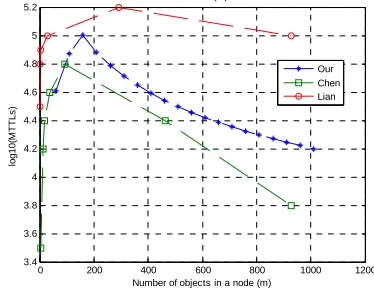
Figure 11 is the comparison result of three models. We can arrive at the following results from Figure 11: 1) moptimal in three models are [103,160,293]. Although the values are not identical, these values are all around B/b=150 and on the same order of magnitude. It indicates that our moptimal is almost the same as in [10] and [11]. 2) The trend of these curves is almost identical.
Although the above analysis shows that our model can draw the similar conclusion as the previous work, there exist three topics to verify our work is significant.
The first topic is why our simpler model can draw similar conclusions. The difference between our model and [11] is the number of failure nodes. We adopt the average number of failure nodes while Chen utilizes the information of the current number of failure nodes in view of node-based-repair. In fact, the average number of failure nodes is the statistical result of all the daily information about the failure nodes, and it is enough to calculate another statistical average value, MTTLS. This is the main reason that our result is almost the same as [11].
0 500
1000 1500
2000 2500
0 1000 2000 3000 4000 50003
3.5 4 4.5 5
X: Number of objects in a node (m) X: 210
Y: 1210 Z: 4.954 MTTLS=f(m,N)
Y: Total number of nodes (N)
log
10(M
T
T
LS
)
Figure 10. MTTLS varies with m and N from system’s view. b=20MB/s, B=3GB/s, S=3PB.
Another topic needs to be discussed is why [10] and [11] does not quantify the impact of the total number of nodes, N. In [10], that is because the repairing rate in this simple node-based-repair model does not include the third item of formula (2) and the number of failure nodes,
Noptimalcan’t be directly figured out. In [11], although the
model might be used to figure out more accurate MTTLS, the complex formula of repairing bandwidth and the dynamic number of repairing nodes make it hard to achieve Noptimal. The state space scale of the model in [11]
is determined by N, so it is hard to calculate Noptimal by
solving the model directly since it is difficult to solve the state matrix when N is very large.
0 200 400 600 800 1000 1200
3.4 3.6 3.8 4 4.2 4.4 4.6 4.8 5 5.2
Number of objects in a node (m)
lo
g1
0(
M
T
T
Ls
)
MTTLs=f(m)
Our Chen Lian
Figure 11. Comparing our model with Chen’s and Lian’s. b=20MB/s, B=3GB/s, S=3PB, N=1024.
The third topic is about the optimal combination of several parameters. This is not discussed either in [10] or [11]. We quantify this combination by optimizing the function of MTTLS, N and m through GA. In general, this result is more practical for designing real-world systems.
VII.RELATED WORK
Data reliability is critical to large scale storage systems. The prior research studied the RAID’s MTTDL in [18] [4], using Markov models with exponentially distributed disk failures. When the idea of RAID has been extended into larger storage systems, in which fault probability is high and repairing rate is a key factor, researchers focus on how to improve data reliability from these two aspects. Our research is in this category.
Q. Xin et.al [4,5] studied the effect of distributed recovery inside a RAID and outside a RAID. They paid little attention to how the replica placement affects the recovery rate. Ramabhadran et.al [6] studied a single object's reliability similar to MTTDLOin Section II.B in long-running replicated system without considering the effect of available repairing bandwidth.
Øystein Torbjørnsen [9] proposed the Q-rot policy and analyzed some factors influencing the system availability based on a node-based-repair Markov model. It mainly discussed the database read/write access impact on the system availability and it is different from our focus.
focuses on not only how the parameters impact the reliability, but also what are the optimal values of the parameters, which educe the best reliability. In addition, another issue, finding the optimal combination value of the parameters but not the individual optimal value, is not discussed in these papers.
VIII.CONCLUSIONS AND FUTURE WORK
Designing a reliable large-scale data warehouse or storage system induces many key challenges. One of them is to figure out some basic system parameters, such as the total number of stored objects, the number of nodes, and the bandwidth of switch and the node. This paper presents a new object-based repair model. By analyzing this model, we work out the individual optimal value of parameters and their optimal combination. These results can provide the engineers with direct instructions to design reliable systems. Our further work will focus on trading off more factors in a large storage system: the cost, IO bandwidth, and reliability, to recommend the best parameters for system designers.
ACKNOWLEDGMENT
This paper is supported by the National Grand Fundamental Research 973 Program of China under Grant No.2005CB321804, the National Science Fund for Distinguished Young Scholar of China under Grant No.60625203, and Program for New Century Excellent Talents in University (NCET-06-0928).
REFERENCES
[1] http://www.businessintelligencelowdown.com/2007/02/top
_10_largest_.html. 2008.
[2] David E. Goldberg. Genetic Algorithms in Search,
Optimization and Machine Learning, 1st edition. Addison-Wesley Longman Publishing Co., Inc. 1989.
[3] S. Ghemawat, H. Gobioff, and S.-T. Leung, “The Google
File System”, in Proc. of the 19th SOSP, 2003.
[4] Q. Xin, E. L. Miller, D. D. E. Long, S. A. Brandt, T.
Schwarz, W. Litwin, “Reliability Mechanisms for Very Large Storage Systems”, in Proc. of 20th IEEE/11th NASA Goddard Conference on Mass Storage Systems & Technologies, Apr., 2003
[5] Q. Xin, E. Miller, T. Schwarz. Evaluation of Distributed Recovery in Large-Scale Storage Systems. Thirteenth IEEE International Symposium on High Performance Distributed Computing, 2004.
[6] S. Ramabhadran, J. Pasquale, “Analysis of Long-Running
Replicated Systems”, in INFOCOM 2006.
[7] “Reference information: The next wave”, The Enterprise Storage Group, June 2002.
[8] Wei Chen. Trends and Challenges in Large-Scale Data
Center Availability. Panel on SRDS 2007.
[9] Øystein Torbjørnsen. Multi-Site Declustering Strategies for Very High Database Service Availability. Phd thesis University of Trondheim, Norway. 1995.
[10]Q. Lian, W. Chen, Z. Zhang, “On the Impact of Replica
Placement to the Reliability of Distributed Brick Sto-rage Systems”, in ICDCS 2005.
[11]Ming Chen, Wei Chen, Likun Liu, and Zheng Zhang. An
Analytical Framework and Its Applications for Studying Brick Storage Reliability. In SRDS 2007.
[12]ADYA, etc. FARSITE: Federated, Available, and Reliable Storage for an Incompletely Trusted Environment. In OSDI (2002).
[13]SANTOS, J., MUNTZ, R., AND RIBEIRO-NETO, B.
Comparing Random Data Allocation and Data Striping in Multimedia Servers. In ACM SIGMETRICS (2000). [14]H. Yu, P. B. Gibbons, and S. Nath, “Availability of
Multi-Object Operations”, in Proc. of NSDI'06.
[15]KISTLER, J. J., AND SATYANARAYANAN, M.
Disconnected Operation in the Coda File System. ACM Transactions on Computer Systems (Feb. 1992).
[16]PATTERSON, D. A., GIBSON, G., AND KATZ, R. H. A
Case for Redundant Arrays of Inexpensive Disks (RAID). In ACM SIGMOD 1988.
[17]R. Billinton, R. N. Allan. Reliability Evaluation of
Engineering Systems: Concepts and Techniques. Plenum Press. 1983. p245-247.
[18]W. A. Burkhard, J. Menon, “Disk Array Storage Sys-tem
Reliability”, in Proc. of Symposium on Fault-Tolerant Computing, 1993.
[19]R VAN RENESSE, KP BIRMAN, W VOGELS.
Astrolabe: A robust and scalable technology for Distributed System monitoring, management, and data mining. ACM transactions on computer systems, 2003.
Kai Du was born in 1978. He received B.E. and M.E. degree in National University of Defense Technology, China. He is currently pursuing PhD degree in NUDT, China. His current research interests include large-scale data management, data reliability, distributed computing.
Zhengbing Hu was born in 1978. He received B.E., M.E. and P.h.D degree in National Technical University of Ukraine. His current research interests include Network Security, Intrusion Detection System, Artificial Immune System, Data Minging etc..
Huaiming Wang was born in 1962. He received B.E. degree in Information Project University of PLA, M.E. and PhD degree in National University of Defense Technology, China. Currently he is professor in school of computer science, NUDT. His current research interests include information security, system reliability, distributed computing.
Yingwen Chen was born in 1979. He received B.E., M.E. and Ph.D. degrees in National University of Defense Technology, China. He is currently a lecturer in School of Computer at NUDT. His current research interests include distributed computing, mobile data management and wireless computing.
Shuqiang Yang was born in 1968. He received B.E. degree in Information Project University of PLA, M.E. and PhD degree in National University of Defense Technology, China. Currently he is professor in school of computer science, NUDT. His current research interests include database, system reliability, distributed computing.