New technique of two numerical methods for solving integral equation of the second kind

ISSN (e): 2250-3021, ISSN (p): 2278-8719

Vol. 08, Issue 9 (September. 2018), ||V (V) || PP 34-40

International organization of Scientific

Research

34 | P a g e

New technique of two numerical methods for solving integral

equation of the second kind

M. A. Abdou

1

, A. A. Abbas

2

Mathematics Department, Faculty of Education, Alexandria University Mathematics Department, Faculty of Science, Benha University

Corresponding Author: M. A. Abdou

Abstract:Here, we use new technique ofTrapezoidal Rule and Simpson's Rule

, as two numerical approximation methods to solve the integral equations of type Fredholm and Volterrs with conuiouskernel.Some numerical examples are considered and the error of the method is computed. Comparizonbetween the solution of ordinary differential and the corresponding solution of integral equation, numerically is obtained.

Key Wards:Volterra integral equation, Trapezoidal Rule, Simpson's Rule, approximate method, the error of

the method.

--- --- Date of Submission: 29-09-2018 Date of acceptance: 14-10-2018 --- ---

I. INTRODUCTION

Many problems of mathematical physics, engineering and contact problemsin the theory of elasticity lead to integral equations (Abdou, 2002; Abdou,131, 2002; Abdou, 2003).Their solutions can be obtained analytically, using the theory developed by (Mushkelishvili,1953). The books edited by (Green,1969); Hochstadt,1971; Golberg.ed,1979 and Tricomi,1985) contain many different methods to solve the integral equations analytically. The book edited by (Golberg.ed,1990) contain extensive literature surveys on both approximate analytical and purely numerical techniques. The interested reader should consult the fine expositions by (Atkinson , 1976, 1997); (Delves and Mohamed,1985) and (Linz,1985) for numerical methods. (Abdou, 137,2003) obtained a Fredholm integral equation of the first kind with singular kernel, when the mixed problem of continuous media with boundary conditions specified on a circle is studied. (Abdou131,2002) obtained and solved the Fredholm integral equation of the second kind, when the kernel takes the Weber–Sonin integral form. The integral equation is investigated, in this case, from the semi-symmetric Hertz problem of two different materials in three-dimensional. Also the resolving of Fredholm integral equation of the second kind, and others cases are studied by (Abdouand Nasr, 2003).

Here, in this paper, we discuss the solution of integral equation using Trapezoidal Rule and Simpson's Rule. Moreover, we compare the numerical results with the corresponding results of ordinary differential equation

II. SOLUTION OF VOLTERRA EQUATION USING TRAPEZOIDAL RULE

To solve Volterra integral equation

( ) ( ) ( , ) ( ) x

a

x g x k x y y dy

  

_

 (1)

numerically by another way that call Trapezoidal rule, we apply the basic formula of the trapezoidal rule , see (Atkinson, 1976, 1997) we obtain

𝑘 𝑥𝑗, 𝑦 ∅ 𝑦 𝑑𝑦 = 𝑕𝑗 𝑥_𝑗

𝑎

(1

2𝑘𝑗 ,0𝑦0+ 𝑘𝑗 ,𝑖𝑥𝑖+ 1 2𝑘𝑗 ,𝑗𝑦𝑗)

𝑗 −1

𝑖=1

+ 𝑔𝑗

, 𝑗 = 1,2,3, … , 𝑁 . (2) Here, in (2), we divide the interval [0, 𝑥] to 𝑁 parts, where we assume

0 = 𝑥0≤ 𝑡1≤ 𝑥2≤ ⋯ ≤ 𝑥𝑖 ≤ ⋯ ≤ 𝑥𝑛 = 𝑥 ;

Also, we wtite

0 0

( n ) / ; , j y ; 1, 2,..., 1.

y x a n y a y a j y j y j n

           

Moreover, to find



( )

x

, we consider

0 0 ; 0

, , 1 1.

n n i i

i i

x y a and x x y x x i y a i y y

i e x y i n

35

Using the following definitions

g x

(

_i

)



g k x

_i

, (

_i

,

y

_j

)



k

_ij

,

we have

0 0 1 1

n-1 1

j

j n

1

( , ) ( ) [ ( , ) ( ) ( , ) ( ) . . . 2

1

k(x,y ) ( ) ( , ) ( )] , 2

y

y , y , j 1 , x x

x

a

n n n

n

k x y y dy y k x y y k x y y

y k x y y

a _{x a}

x y

j n

  

 _ 

   

 

 

      



(3)

III. SOLUTION OF VOLTERRA EQUATION USING SIMPSON'S RULE :

Consider Simpson's Rule

 

( / 2) 1 / 2

2 2 1

1 1

( ) [ ( ) 2 ( ) 4 ( ) ( )] 4 3

x n n

i i

i i

a

h

A f y dy f a f x f x f x





 



_

 









Using the result of (3) in (1) we have the approximate solution of (1), for

a

 

y

x.

While, the solution

(x)=0,

y>x.





The error of the method can be obtained from the term (n+1).

As the previous section, we divide interval [𝑎, 𝑥] into 𝑁 segment, rewrite the integral term of (1) with x = xi,

where 0 = x0< x1< ⋯ < xi< ⋯ < x𝑁= x, to get

i

ij ,

0 j 0

i

( , ) ( ) ( , ) ( ) h w ( ) ( ( , ), ( ))

{ , h (x-a)/n , x , i 2,3,...,n}

i

x _i

i ij i j j ij j i y i

j a

i i

k x y y dy h w k x y y k y E k x y y

x x a ih y

   

 

  

     







₍₅₎

Where,

w

_ij represent the weight function, while

E

_{i y,}

( (

k x

_i

, ), ( ))

y



y

is the error function. With the aid of Simpson’s third rule and Days rule, we get

0

[ , ] , r 2 ,4 , 6,... 3

r

r r rj j

j h

g w k rh jh







 



 (6)

IV. ANALYSIS OF THE ERROR

Consider the integral equation

( )

( )

( , ) ( )

, 0

t

T

1

t

a

t

f t

k t s

s ds

















(7)

Using a numerical method, we have

0

( , ) ( ) ( , ) ( ) ( , ) ( )

n n

t

t t

n ni n i i

i

a a

k t s s ds k t s  s ds h w k t t  t 

 







(8)

The transformation from integral formula to an algebraic formula, we have a local error

0

( , )

( , ) ( )

b _n

n n in in i

i a

E h t

k t s



s ds

h

w k















(9)

The local error depends on its calculations on two important bases: A) Measuring accuracy in the vicinity of the given function. B - the base of numerical integration used.

1 Estimation of error and numerical stability:

If the numerical solution grows and slowly increases when compared to error i.e, there is constant error or a slight increase is not comparable to the increase in numerical solution to the exact solution), the method used is poor. On the contrary, the error may increase more rapidly than the numerical solution approaches the exact solution. Therefore, this phenomenon is called numerical instability and this phenomenon is very well known when solving normal differential equations. We will show that this phenomenon also applies when solving integral equations.

Consider the exact solution



and





is the numeric solution. Hence, the error formula is

36

Subtracting the numerical solution from the exact solution, we get

( ) ( ) ( , )[ ( ) ( )] ( ) b

a

t t k t s s s ds E t

  

_

   (11)

Hence, the integral equation of the computational error

( ) ( , ) ( ) ( ) b

a

e t 



k t s e s dsE t (12) Here, the known functions represent the kernel and the function of transformation.

Let the integral operator of the error is

( , ) ( )

b

a

Ke





k t s e s ds

Then, we have

1

1

( ) ( ) (1 )

(1 ) E , det(1-K) 0

1

(1 ) 1.

(1 )

e t Ke E t K e E

e K K K K                 

V. SOME NUMERICAL EXAMPLES

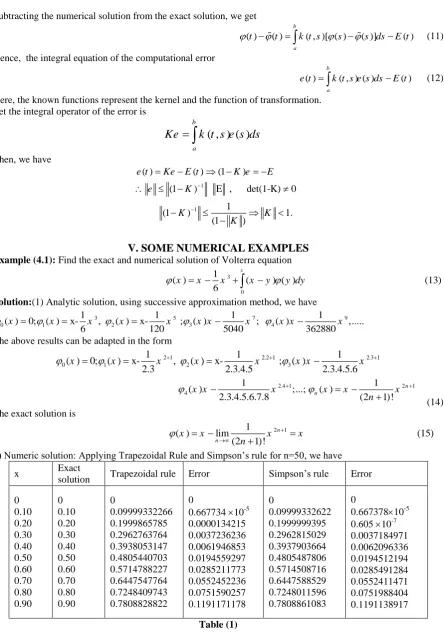
Example (4.1): Find the exact and numerical solution of Volterra equation

3

0

1

( ) ( ) ( ) (13) 6

x

x x x x y y dy

   

_

 

Solution:(1) Analytic solution, using successive approximation method, we have

3 5 7 9

0 1 2 3 4

1 1 1 1

( ) 0; ( ) x- , ( ) x- ; ( ) ; ( ) ,...

6 120 5040 362880

x x x x x x x x x x x

         

The above results can be adapted in the form

2 1 2.2 1 2.3 1

0 1 2 3

1 1 1

( ) 0; ( ) x- , ( ) x- ; ( )

2.3 2.3.4.5 2.3.4.5.6

x x x x x x x x



_



_ 



_ 



_ 

2.4 1 2 1

4

1 1

( ) ;...; ( )

2.3.4.5.6.7.8 (2 1)!

n n

x x x x x x

n

 _   _{ } 



(14) The exact solution is

2 1

1

( ) lim (15) (2 1)!

n n

x x x x

n







  



2) Numeric solution: Applying Trapezoidal Rule and Simpson’s rule for n=50, we have Error Simpson’s rule Error Trapezoidal rule Exact solution x 0

0.66737810-5 0.605 10-7 0.0037184971 0.0062096336 0.0194512194 0.0285491284 0.0552411471 0.0751988404 0.1191138917 0 0.09999332622 0.1999999395 0.2962815029 0.3937903664 0.4805487806 0.5714508716 0.6447588529 0.7248011596 0.7808861083 0

0.667734 10-5 0.0000134215 0.0037236236 0.0061946853 0.0194559297 0.0285211773 0.0552452236 0.0751590257 0.1191171178 0 0.09999332266 0.1999865785 0.2962763764 0.3938053147 0.4805440703 0.5714788227 0.6447547764 0.7248409743 0.7808828822 0 0.10 0.20 0.30 0.40 0.50 0.60 0.70 0.80 0.90 0 0.10 0.20 0.30 0.40 0.50 0.60 0.70 0.80 0.90 Table (1)

37

The relation between the exact and numeric solution (Trap. rule). In addition, the error is computed

The relation between the exact and numeric solution (Sim. rule). In addition, the error is computed

Example (2): Consider the Volterra integral equation 𝜙 𝑡 + 𝑒𝑥+𝑡

𝑡

0

𝜙 𝑠 𝑑𝑠 = 𝑒2𝑡_{(𝑡 − 2)}2_{− 4𝑒}𝑡_{+ 𝑡}2_{− 2𝑡, (16)}

It is difficult to obtain, directly the exact solution, using the classical famous methods. Therefore,write equation (16), in the form

𝑢 𝑡 =𝑓 𝑡

𝑃 𝑡 − 1

𝜐 𝑡 𝜐 𝑠 𝑓 𝑠

𝑃 𝑠 𝑑𝑠 𝑡

0 (17)

Here,

𝑢 𝑡 =𝑒

2𝑡 _{𝑡 − 2} 2_{− 4𝑒}𝑡_{+ 𝑡}2_{− 2𝑡}

𝑒𝑡 −

1

𝜐 𝑡 𝜐 𝑠

𝑒2𝑠_{(𝑠 − 2)}2_{− 4𝑒}𝑠_{+ 𝑠}2_{− 2𝑠}

𝑒𝑠 𝑑𝑠

𝑡

0

. (18) The integrating factor

𝜐 𝑡 = 𝑒𝑥𝑝 𝑃 𝑠 𝑄 𝑠 𝑑𝑠 = exp 𝑒2𝑠_{𝑑𝑠 = exp} 𝑒 2𝑠

38

𝜙 𝑡 = 𝑒2𝑡 _{𝑡 − 2} 2_{− 4𝑒}𝑡_{+ 𝑡}2_{− 2𝑡 −}

exp −𝑒

2𝑡

2 exp 𝑒2𝑠

2 𝑒

𝑠 _𝑒2𝑠_{(𝑠 − 2)}2_{− 4𝑒}𝑠_{+ 𝑠}2_{− 2𝑠 𝑑𝑠} 𝑡

0

. (19) It is not easy to calculate the latter integration, so, we solve the Volterra integral equation (16) numerically, then an integral part of equation (19) is solved as a part of solving differential equation to find the value of 𝜙 𝑡 . In both we use the famous methods, Trapezoidal method and modified Simpson rule in various times.

At t=0.13

The solution of integral equation

x Exact App. Trap. Error Trap. App. Simp. Error Simp.

0 0 0 0 0 0

0.013 -0.025831 -0.0258881 5.71489E-05 -0.02587382 4.28228E-05 0.026 -0.051324 -0.0514398 1.15759E-04 -0.05141051 8.65118E-05 0.039 -0.076479 -0.0766548 1.75817E-04 -0.07661005 1.31051E-04 0.052 -0.101296 -0.1015333 2.37306E-04 -0.10147239 1.76395E-04 0.065 -0.125775 -0.1260752 3.00207E-04 -0.12599751 2.22505E-04 0.078 -0.149916 -0.1502805 3.64497E-04 -0.15018535 2.69348E-04 0.091 -0.173719 -0.1741491 4.30150E-04 -0.17403587 3.16870E-04 0.104 -0.197184 -0.1976811 4.97136E-04 -0.19754903 3.65030E-04 0.117 -0.220311 -0.2208764 5.65421E-04 -0.22072478 4.13777E-04 0.13 -0.2431 -0.243735 6.34970E-04 -0.24356304 4.63041E-04

Table (2)

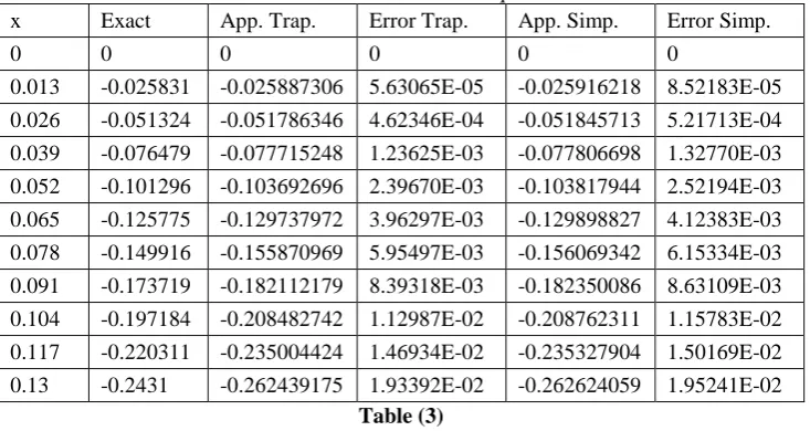
The numerical solution of the integral equation (16) using Trapezoidal rule and Simpson’s rule The solution of differential equation

x Exact App. Trap. Error Trap. App. Simp. Error Simp.

0 0 0 0 0 0

0.013 -0.025831 -0.025887306 5.63065E-05 -0.025916218 8.52183E-05 0.026 -0.051324 -0.051786346 4.62346E-04 -0.051845713 5.21713E-04 0.039 -0.076479 -0.077715248 1.23625E-03 -0.077806698 1.32770E-03 0.052 -0.101296 -0.103692696 2.39670E-03 -0.103817944 2.52194E-03 0.065 -0.125775 -0.129737972 3.96297E-03 -0.129898827 4.12383E-03 0.078 -0.149916 -0.155870969 5.95497E-03 -0.156069342 6.15334E-03 0.091 -0.173719 -0.182112179 8.39318E-03 -0.182350086 8.63109E-03 0.104 -0.197184 -0.208482742 1.12987E-02 -0.208762311 1.15783E-02 0.117 -0.220311 -0.235004424 1.46934E-02 -0.235327904 1.50169E-02 0.13 -0.2431 -0.262439175 1.93392E-02 -0.262624059 1.95241E-02

Table (3)

The numerical solution of the differential equation (19) using Trapezoidal rule and Simpson’s rule

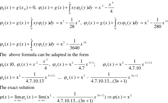
Example (3): Find the exact and numerical solution of Volterra equation

5 2

0

( ) ( )

4 x x

x x xy y dy

   

_



39

5 2

0 0 1 0

0

2 8 2 11

2 1 3 2

0 0

( ) ( ) 0, ( ) ( ) ( )

4

1 1

( ) ( ) ( ) x , ( ) ( ) ( ) x

28 280

x

x x

x

x g x x g x xy y dy x

x g x xy y dy x x g x xy y dy x

                    







2 14 4 3 0 1

( ) ( ) ( ) x 3640

x

x g x xy y dy x



 





 

The above formula can be adapted in the form

5

2 2 5 3 2 5 3.2

0 1 2 3

2 5 3.3 2 3 2

4

1 1

( )0, ( ) , ( ) x ; ( ) x

4 4.7 4.7.10

1 1

( ) x ... ( ) x -

4.7.10.13 4.7.10.13...(3 1)

n n

x

x x x x x x x

x x x x

n                    

The exact solution

2 1 3 2 2

( ) lim ( ) lim(x - ) ( ) x 4.7.10.13...(3 1)

n n

n n

x x x x

n

   

 

   



(2) Numeric solution: Applying Trapezoidal Rule and Simpson’s rule for n=50, we have Error Simpson's rule Error Trapezoidal rule Exact solution x 0

0.19876 10-6 0.73 10-9 0.00058456743 0.0022516058 0.0077462541 0.0186863338 0.04181522872 0.0805949288 0.1474315277 0 0.01000019876 0.03999999927 0.08941543257 0.1577483942 0.2422537459 0.3413136662 0.4481088633 0.554050712 0.6625684723 0

0.10002 10-6 0.80130 10-6 0.00058814749 0.0022196158 0.0077562108 0.0186168661 0.0419097933 0.0804808855 0.1474593718 0 0.0100010002 0.0400080130 0.08941185251 0.1577803842 0.2422437892 0.3413831339 0.4480902067 0.5595191145 0.6625406282 0 0.0100 0.0400 0.0900 0.1600 0.2500 0.3600 0.4900 0.6400 0.8100 0 0.10 0.20 0.30 0.40 0.50 0.60 0.70 0.80 0.90 Table (4)

The numeric results for the exact solution, Trap rule andSimp. rules with error in each case

40

The relation between the exact and numeric solution using Simp.Rule, with the error.

VI. CONCOLUSION

REFERANCES

[1]. Abdou, M. A.(2002), FredholmــVolterra integral equation of the first kind and contact problem, J. Appl. Math. Comput.125 177ــ193.

[2]. Abdou, M. A. (2002), FredholmــVolterra integral equation and generalized potential kernel, J. Appl. Math.Comput.131, 81ــ94.

[3]. Abdou, M. A. (2003), On asymptotic methods for FredholmــVolterra integral equation of the second kind in contact problem, J. Comp. Appl. Math. 154, 431ــ446.

[4]. Muskhelishvili, N. I .(1953), Singular Integral Equations, Noordhoff, Groningen, The Netherland, . [5]. Green, C.D.(1969) Integral Equation Methods, New York,.

[6]. Hochstadt,H. (1971) Integral Equations, Awiley Inter Science Publication, New York,. [7]. Golberg.ed.M.A(1979), Solution Methods for Integral Equations, New York,.

[8]. Tricomi, F.G. (1985) Integral Equations, Dover, New York.

[9]. Golberg.ed.M.A(1990), Numerical Solution for Integral Equations, NewYork.

[10]. Atkinson,K.E(1976), A Survey of Numerical Method for the Solution of Fredholm Integral Equation of the Second Kind, Philadelphia.

[11]. Atkinson,K.E(1997),The Numerical Solution of Integral Equation of the Second Kind, Cambridge University, Combridge.

[12]. Delves, L.M. and J.L.Mohamed,J.L.(1985), Computational Methods for Integral Equations, NewYork, London.

[13]. Peter Linz, (1985), Analytic and Numerical Methods for Volterra Equations, SIAM, Philadelphia. [14]. Abdou, M. A. (137-2003), FredholmــVolterra integral equation with singular kernel, J. Appl. Math.

Comput.231ــ243.