Regularized Least Squares Estimating
Sensitivity for Self-calibrating Parallel Imaging
LIU Xiao-fang
College of Computer Science and Technology, Zhejiang University, HangZhou, China Department of Biomedical Engineering, China Jiliang University, HangZhou, China
Email: [email protected]
YE Xiu-zi and ZHANG San-yuan
College of Computer Science and Technology, Zhejiang University, HangZhou, China
LIU Feng
School of Information Technology & Electrical Engineering,The University of Queensland, Brisbane, Australia
Abstract—Calibration of the spatial sensitivity functions of
coil arrays is a crucial element in parallel magnetic resonance imaging (pMRI). The self-calibrating technique for sensitivity extraction has complemented the common calibration technique that uses a separate pre-scan. In order to improve the accuracy of sensitivity estimate from small number of self-calibrating data, which is extracted from a fully sampled central region of a variable-density k-space acquisition in self-calibrating parallel images, a novel scheme for estimating the sensitivity profiles is proposed in the paper. On consideration of truncation error and measurement errors in self-calibrating data, the issue of calculating sensitivity would be formulated as a regularized least squares estimation problem, which is solved by the preconditioned conjugate gradients algorithm. When applying the estimated coil sensitivity to reconstruct full field-of-view(FOV) image from the under-sampling simulated and in vivo data, the normalized signal-to-noise ratio (NSNR) of reconstruction image is evidently improved, and meanwhile the normalized mean squared error (NMSE) is remarkably reduced, especially when a rather large accelerate factor is used.
Index Terms—parallel magnetic resonance imaging (pMRI),
self-calibrating technique, regularized least squares (RLS), preconditioned conjugate gradients (PCG), generalized encoding matrix(GEM) reconstruction
I. INTRODUCTION
Parallel magnetic resonance imaging (pMRI) is a rapid acquisition technique and considered to be one of the modern revolutions in the field of MRI. The technique simultaneously samples the reduced k-space data and uses the information from multiple receivers to reconstruct full Field-Of-View (FOV) image. In parallel imaging, since a certain amount of the spatial encoding, traditionally achieved by the phase-encoding gradients, is substituted by evaluating data from several coil elements with spatially different coil sensitivity profiles, the choice of sensitivity calibration strategy is at least as important as the choice of reconstruction strategy [1].
Unfortunately, the existing techniques for determining sensitivity functions are not satisfactory. The most common technique has been to derive sensitivities directly from a set of reference images obtained in a separate calibration scan before or after the accelerated scans. This calibration step can prolong total examination time, partially counteracting the benefits of decreased acquisition time associated with PMRI. Meanwhile, it also introduces a possible source of error into the PMRI reconstruction, as it is difficult to ensure that the patient and coil array will be in the same positions during both the calibration scans and the accelerated data acquisitions. Adaptive sensitivity estimation is another technique for determining sensitivity functions, which is a major concern in dynamic imaging applications. Based solely on the data from accelerated scans, the method uses “unaliasing by Fourier-encoding the overlaps using the temporal dimension” (UNFOLD) [2] to generate low-temporal-resolution, aliasing-free reference images for sensitivity estimation. However, UNFOLD is limited to dynamic applications in which at least half FOV remains static over time.
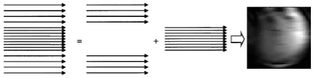
A more general method is the self-calibrating technique, which also eliminates a separate calibration scan but acquires variable-density k-space data during the accelerated scan [3,4]. In addition to the down-sampled lines at outer k-space, the variable-density acquisition includes a small number of fully sampled lines at the center of k-space, known as auto-calibration signal (ACS) lines in generalized auto-calibrating partially parallel acquisitions (GRAPPA) [5], namely self-calibrating lines. These self-calibrating lines after Fourier transformation produce low-resolution reference images
as
[ ( ) ( )]
low resolution l
f r c r
r
r
for any given component coil l, where “low-resolution” superscript indicates that use of only the central k-space positions, that results in a
Figure 1. A sample variable-density k-space trajectory made up of a regularly under-sampled outer portion and a fully sampled inner portion. The inner portion may be used as a low-resolution sensitivity reference for PMRI reconstructions.
resolution measurement of the product of the image of transverse magnetization f(
r
r
) and the coil sensitivity cl(r
r
).To derive the sensitivities, these low-resolution reference images are divided by their sum-of-squares(SoS) combination[3,6,7]:2
[ ( ) ( )]
ˆ ( )
|[ ( ) ( )]
|
low resolution l
l low resolution
l l
f r c r
c r
f r c r
r
r
r
r
r
(1) In general, the approximation in Eq.(1) requires the range of spatial frequencies cover in the self-calibrating lines is much broader than the spatial frequency band of the coil sensitivity functions[8]. However, this increase the acquisition time associated with pMRI and contradicts the goal of pMRI. If a small number of self-calibrating lines are used, truncation of high spatial frequency components of transverse magnetization f(
r
r
) results in Gibbs ringing artifacts in the extracted sensitivity reference images. These ringing errors become serious especially at locations where the object transverse magnetization has high-spatial-frequency components. However, these Gibbs ringing errors in reference images cannot be canceled by the division of their SoS combination as Eq.1, and can hardly be reduced by the commonly used polynomial-fitting[9] or wavelet-denoising [10] techniques for sensitivities. Consequently, the pMRI reconstruction interprets varying degrees of Gibbs ringing as actual features of the sensitivities, and corresponding sensitivity-mismatch artifacts can result. Therefore, to improve the sensitivity accuracy with a small number of self-calibrating lines is crucial for pMRI to achieve a high acceleration.Towards quieter and faster imaging, the paper would study the method for improving the accuracy of sensitivity estimate from small number of self-calibrating data, and the quality of reconstruction images would be used to evaluate the effectiveness of the proposed method. Using only the self-calibrating data in a variable-density acquisition, a novel method for estimating the sensitivity profiles would be proposed in the paper. On consideration of Gibbs ringing artifacts and noise in sensitivity reference images, which is generated from self-calibrating data, this method would view the issue of estimating cl(
r
r
) from these images as a linear estimation problem, and regularized least-squares methods are used to estimate the sensitivity profiles. In order to obtain the stable solution, the conjugate gradients algorithm, together with an acceleration scheme as circulant preconditioner, is used to solve this estimation problem. In the paper, the suitable number of self-calibrating central lines for generating the sensitivity reference images would also be discussed. In combination with the generalized encoding matrix (GEM) reconstruction [11] method, the effectiveness of this self-calibration method would be demonstrated via phantom and in vivo brain imaging study.
II. THEORY AND METHODS
A. Figures and Formulation of sensitivity estimation in self-calibrating parallel imaging
To improve SNR and reduce acquisition times, the use of multiple receive coils has become increasingly popular in MRI. Let cl(
r
r
) denote the sensitivity of the lth coil, for l=1, . . . , L, where L denotes the number of coils. Let
yl(
r
r
) denote the recorded measurements associated with the lth coil, then the general forward model for the MR measurement signal associated with the lth coil is :
( )
( ) ( )
ik r1,...
l l l
y r
c r
r e dr
l
L
r rr
r
r
r
(2) Where ρ(
r
r
) denotes the object’s transversemagnetization;
k
r
is the chosen k-space trajectory indices
(e.g.,
k
r
≡(kx, ky)) representing a total number of acquired data points measured in the presence of various frequency- and phase-encoding gradients. The measurement errors εlare modeled by additive, complex,
zero-mean white gaussian noise [12,13,14].
With only a modest loss of generality[15], the integral in Eq. (2) may be approximated with a discrete sum:
( )
( )
( )e
ik r( )
( )
l l l
r
y k
c r
r r
r
r
r
r
r
r
r
(3) Here the vector index
r
r
in the sum indicates a summation over all discrete pixel positions in the image. Simplifies Eq.(3) and yields the following matrix-vector equation:yl=clρ+εl (4)
For coil sensitivity varies slowly as a function of dominant spatial variations position, low-resolution in-vivo images suffice to form sensitivity references data [16]. In self-calibrating parallel imaging, the variable-density data acquisition schemes are usually adopted (see Fig.1). Here, k-space is effectively split into two regions: a central region in which all phase-encode lines are fully sampled, and an outer region in which the lines are uniformly under-sampled.
The central lines of k-space are extracted and Fourier transformed to yield low-resolution reference images as the measurement data of sensitivity reference ylreference.
According to Eq.(4), the following equation would be proposed in the paper:
( ) ( )
refrence low resolution
l l l
y rr
c r er (5) Here, eldenotes any error, such as truncation error and
measurement errors. Aiming at estimating sensitivity profiles, ρlow-resolution would be calculated by the
sum-of-squares (SoS) combination of these reference images, which can be the low-resolution reconstruction image and noted as G in the paper. At last, the following model would be used to calculate the sensitivity profiles:
yl=Gcl +el (6)
As shown in Eq.(6), a certain approaches might be taken to remove the magnetization distribution and isolate the encoding effects of pure coil sensitivities.
B. References Regularized least-squares estimation of coil sensitivity maps
Because cl appears linear scaling in Eq.(6), the
problem of estimating cl would be a linear estimation
problem, which can be resolved by minimizing the following regularized least-squares cost function:
2
ˆ
arg min ( )
1
( )
||
||
( )
2
2
l
l l
c reference
l l l l
c
c
c
y
Gc
R c
(7) Where ĉl denotes the estimation values of cl, and
ylreference denotes the sensitivity reference images; R(cl) is
regularizing roughness penalty functions that encourages piecewise-smooth estimates, and β is regularized parameters that control the smoothness of the estimates. Thus, our goal is to compute an estimate ĉl of cl from by
finding the minimum of the objective function Ф(cl).
In Eq.(7), an open problem is how to best choose the regularizer R(cl). If this term is not included, then the
sensitivity estimate ĉl will suffer from noise and Gibbs
ringing artifacts because this inverse problem is ill-conditioned. The simplest choice is Tikhonov regularization, another choice is a quadratic roughness penalty function, which penalizes differences between neighboring pixel values. The following regularizing penalty function would be used in this paper:
1
( )
l K k([
l k] )
kR c
Dc
(8) Where φ is a convex potential function, and K is the number of pairs of neighboring pixels; D is a K×ndmatrix,
and each row of D contains one "+1" and one "-1" entry so that [Dcl]k corresponds to the difference between two
neighboring pixel values. For coil sensitivity is assumed smooth, the quadratic potential function φ(t)=t2/2 would
be adopted and second-order differences are used for all results in our study. The quadratic potential function is convenient for minimization [17], but it has the drawback of smoothing image edges, particularly if the regularization parameter β in Eq. (7) is too large.
C. Minimization using preconditioned conjugate gradients algorithms
Under the above assumptions, we can determine the unique minimizer ĉl of the cost function Ф(cl) by finding
the zero of its gradient. For differentiable regularizers, the gradient of Ф(cl) is expressed as:
' ( )
c
lb Hc
l
(9)Where H is the Hessian matrix of Ф(cl); H=G′G+βD′D;
b G≌ ′ylreference is essentially a “back projection” of
ylreference; ′ and are respectively the conjugate and
gradient operators.
For the quadratic penalty, the zero of the gradient is “simply” the solution of the linear system of equations H ĉl =b. However, due to the size of H for realistic image
sizes, we cannot compute directly the analytical solution. Thus, the iterative methods as preconditioned conjugate gradients (PCG) algorithm would be used to computeĉl.
For quadratic objectives, preconditioning the CG algorithm is equivalent to solving the transformed linear system of equations M1/2HM1/2M-1/2ĉ
l = M1/2b, where M
is the preconditioner matrix. The ideal preconditioner would be M=H-1 because the convergence rate of the CG algorithm generally improves as the condition number of MH decreases toward unity. Since we cannot compute H-1 for large nd pixels, the circulant preconditioner is put forward to approximate H-1, which defined as
M T≌ ′Q′Ω1(β)QT[18], where the matrix T is the identity
matrix; Q is the orthonormal version of the 2-D discrete Fourier transform (DFT) operator, and Ω(β) is a diagonal matrix for any β such that: Hl≈T′Q′Ωl(β)QT. In general, Ω consists of the 2-D DFT coefficients of the column of H corresponding to the pixel at the center of the image.
D. Post-processing
As mentioned earlier, system of Eq. 7 is underdetermined and only the “low-resolution” of SoS reconstruction image is used to calculate the sensitivity profile, so that the reconstruction image is not necessarily identical to a typical SoS reconstruction image, especially when the sensitivity profiles estimated by Eq. (7) with different regularization parameters are used. This difference manifests itself as slight changes in intensity distribution. By multiplying the reconstruction image with the root of the sum of squares of the estimated coil sensitivities and dividing the coil sensitivities by the same quantity, this difference can be removed in a simple step. Although not strictly necessary, this post-processing is useful when calculating the normalized mean squared error (NMSE) of the reconstruction images with the SoS of full images as the gold standard. Nevertheless, it is not necessary for this post-processing when the normalized signal-to-ratio(SNR) of reconstruction images is used to quantitatively evaluate the proposed method.
A. Data Acquisition
Unaccelerated anatomical images of a standard resolution phantom were obtained from a 3T (Siemens Medical Solutions) human using an 8-channel head array coil. Imaging parameters: echo time (TE)=3.45ms, repetition time (TR)=2530ms, T1=1100 ms, Flip angle=7deg, slice thickness=1.33mm, FOV=256*256 mm. The B1 coil maps were calculated using Biot-Savart's law, and the fully sampled k-space data were obtained by inverse Fourier transforming the acquired unaccelerated images.
A in-vivo fully sampled brain dataset was obtained from PULSAR(a matlab toolbox for parallel MRI) [19], which was acquired using MR systems with eight-channel head array and multi-eight-channel receiver from a healthy male volunteer with fast spoiled gradient-echo sequence, TR/TE =300/10 ms, matrix size = 256×256, tip angle=15° and FOV = 22*22 cm.
To simulate the under-sampled datasets in the manner of traditional variable-density data acquisition, the acquired full-sampled k-space data was decimated using reduction factors, namely accelerated factor R=2, 3, 4 and 5 for simulated and in vivo dataset. Meanwhile, the central k-space data were fully sampled to generate the sensitivity reference images. The number of central lines along phase-encode was chosen between 6 and 32.
B. Analysis
The accuracy estimation of coil sensitivity is a major determinant of the quality of parallel magnetic resonance image reconstructions. Self-calibration parallel imaging techniques can eliminate the need for an external sensitivity reference, making reconstruction image less susceptible to miscalibration and image degradation. However, in self-calibration parallel imaging, the sensitivity profiles calculated by Eq.(1) might have the information of transverse magnetization distribution, Gibbs ringing and noise from the data acquisition, and result in the degradation of reconstruction image. In order to improve the accuracy of coil sensitivity estimation, we propose the regularized least-squares method to estimate the coil sensitivity profiles from the reference images, and image reconstructions are implemented by GEM reconstruction method in the MATLAB programming language to test our method.
For the regularized least squares method, choosing the regularization function was a key problem. According to the characteristics of sensitivity function, we would adopt a quadratic differentiable penalty function. For regularized least squares estimating sensitivity profiles is a large linear estimation problem, direct solution methods like the Cholesky factorization are not practical. In this case, an iterative technique known as the conjugate gradient (CG) method, together with an acceleration scheme circulator preconditioning, provides us a very efficient means of solving this linear system [18,20].
In order to comparative evaluation, two sets of coil sensitivity profiles would be used in our study. One set of coil sensitivity profiles is called rough sensitivity map, which are directly estimated from the internal reference
images by Eq.(1); The other set is called RLS sensitivity maps, which are estimated by PCG algorithm to resolve Eq.(7). They would be used to reconstruct full FOV images, and the quality of reconstruction image would be target for evaluating the accuracy of estimated sensitivity profiles. In order to quantitative analyze the quality of reconstruction image, signal-to-noise ratio (SNR) and the normalized mean squared error (NMSE) of image would be calculated. However, we would never explicitly calculate the pure sensitivities in the self-calibrating reconstruction. For the purposes of comparative evaluation, we are interested in determining SNR normalized relative to an optimal image from the corresponding un-accelerated acquisition, so the so-called pixel-to-pixel normalized SNR would be used as Eq.10 in the paper.
1/2 2 1/2 1 2 1/2 ,
1
( )
(
) ( |
( )| ) ( |
| )
l l
normalised
full
reference l
acquired r k
l k
SNR
r
N
f
r
c
N
rrr
r
r
)
(10) Here, Nfull, Nacquired represent the un-accelerated and
accelerated number of phase-encoded lines respectively.
ylreference denotes a low-resolution reference image in a
given component coil l, which is Fourier transformation of the central k-space lines. ĉl represents the coil
sensitivity profiles calculated as introduced before. It
could be seen that
2 1/2 1 2 1/2 ,
( |
( ) | ) ( |
| )
l l
reference
l r k
l k
f
r
c
rrr
r
)
is so-called the geometrical noise multiplication factor, or “g-factor”.
NMSE is defined as the normalized difference square between the reconstructed image and the standard image
fstandard, which was the SoS combination of unaccelerated
images:
an
an
2
2
||
( ) | |
( ) ||
|
( ) |
reconstructed st dard
st dard
r
r
f
r
f
r
NMSE
f
r
r
r
r
r
r
(11) This definition is equivalent to the artifact power (AP), and a higher value of NMSE (or AP) represents reduced image quality, which suggests both increased image artifacts and noise.
IV. RESULTS
A. Simulated results
Figure2. Reference images and sensitivity profiles of individual receiver coil. Here, the reference images are extracted from central k-space data and number of central lines was 16. From reference images, rough sensitivity profiles and RLS sensitivity profiles are estimated by Eq.(2) and Eq.(7) respectively. For RLS sensitivity profiles, iterative order=8, regularized parameter β=4, the quadratic potential function φ(t)=t2/2,
different order=2.
Figure 3. The first row shows the reconstruction images from a set of eight-channel under-sampling data using (a) simulated b1 maps (b) rough sensitivity profiles (c) RLS sensitivity profiles. Here, the reduction factor R was 4.Their pixel-to-pixel normalized SNR maps are also showed on the second row.
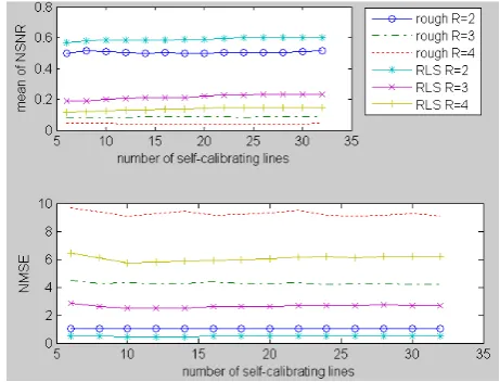
Figure 4. (a) Mean normalized SNR and (b)NMSE of reconstruction images. Here, rough denotes rough sensitivity; RLS denotes RLS sensitivity profiles. They are extracted from 6 to 32 self-calibrating lines respectively, and reconstruction images from under-sampling data when accelerated factor R is 2, 3, 4.
where regularizing penalty function R(cl) adopts a convex
differentiable function for quadratic penalizing second finite differences of cl. RLS sensitivity profiles in Fig.2
are obtained after 8 orders iterative, and the initial guess for iterative procedure is the edge of reference images detected by Canny method.
Using the coil sensitivity maps shown as Fig.2, full-FOV images are reconstructed from the uniform under-sampling data by GEM reconstruction method. Fig.3 shows the reconstruction images and their pixel-to-pixel normalized SNR maps when acceleration factor 4 is used.
With the SoS of full images as the gold standard, Table.1 lists mean of normalized SNR and NMSE of reconstruction images respectively using B1 maps, rough sensitivity profiles and RLS sensitivity maps shown in Fig.2. In Table 1, rough sensitivity maps and RLS sensitivity maps are estimated from 16 self-calibrating lines data. Using these RLS sensitivity maps, the standard deviation of normalized SNR of reconstruction images from under-sampling data of reduction factor R= 2, 3, 4 and 5 are 0.0831, 0.1295, 0.1063 and 0.0557 respectively. As a self-calibrating technique, the suitable number of central k-space phase-encoding lines for generating the
internal sensitivity reference images is also studied in the paper. In Fig. 4a and b, the mean of normalized SNR and NMSE of reconstruction images from the different under-sampling data are plotted as a function of the number of self-calibrating data lines. Fig.4a shows mean of normalized SNR of the reconstruction images which use the rough sensitivity and RLS sensitivity profile, while Fig.4b shows NMSE of reconstruction images. As seen in Fig.4, mean of normalized SNR of the reconstruction
images is improved, and NMSE of reconstruction images is remarkably reduced.
B. In vivo study results
Fig.5 shows the reference images, rough sensitivity maps and RLS sensitivity profiles of eight receiver coils respectively for in vivo study. In Fig.5, the reference images are extracted from the fully-sampled data in 16 central k-space lines along phase encoding direction. From the reference images, the rough sensitivity maps are calculated by Eq.(1), and RLS sensitivity profiles are estimated by Eq.(7), which is resolved by iterative method PCG algorithms as above simulated study.
Table I
Normalized SNR and NMSE of reconstruction images in phantom study
B1 COIL MAPS ROUGH SENSITIVITY RLS SENSITIVITY
R
Mean of NSNR
NMSE
Mean of NSNR
NMSE Mean
of NSNR
NMSE
2 0.5312 1.0000 0.4981 1.0096 0.5865 0.4775 3 0.0837 4.2017 0.0859 4.3606 0.2128 2.6059
4 0.0455 9.0000 0.0400 9.1678 0.1368 5.9173
5 2.1865
e-004 695.9739 2.6217e-004 214.1697 0.0315 15.9599
Figure 5. Sensitivity profiles of eight receiver coil. (a) The sensitivity reference images extracted from 16 self-calibrating lines. From these reference images, (b) Rough sensitivity profiles estimated by Eq.(1); (c) RLS sensitivity profiles estimated by Eq.(7), which is solved by the same method as RLS sensitivity in Fig.2.
Figure 6. The first row shows in vivo reconstruction images using RLS sensitivity profiles in Fig.4, which from the under-sampling data when accelerated factor R is 2, 3, 4 respectively. The second row shows their pixel-to-pixel normalized SNR maps as (a) (b) (c).
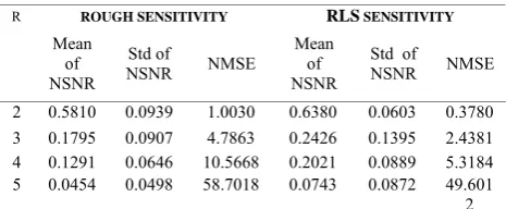
Table II
NSNR and NMSE of reconstruction images in in-vivo study
R ROUGH SENSITIVITY RLS SENSITIVITY
Mean of NSNR
Std of
NSNR NMSE
Mean of NSNR
Std of
NSNR NMSE
2 0.5810 0.0939 1.0030 0.6380 0.0603 0.3780 3 0.1795 0.0907 4.7863 0.2426 0.1395 2.4381 4 0.1291 0.0646 10.5668 0.2021 0.0889 5.3184 5 0.0454 0.0498 58.7018 0.0743 0.0872 49.601 2
R, NMSE, Rough sensitivity, RLS sensitivity, NSNR: definitions as Table.1; Std: standard deviation
Figure7. (a) Mean normalized SNR and (b)NMSE of reconstruction images. Here, rough denotes rough sensitivity; RLS denotes RLS sensitivity profiles. They are extracted respectively from 6 to 32 self-calibrating lines, and reconstruction images from under-sampling data when accelerated factor R is 2, 3, 4.
Using the rough sensitivity profiles and RLS sensitivity shown in Fig.5, the full-FOV MR images reconstructed from the under-sampled in vivo data by GEM reconstruction method are shown in Fig.6, when reduction factor R=2,3,4 is used.
Using rough sensitivity and RLS sensitivity profiles as shown in Fig.5, Table.2 list mean of the normalized SNR and NMSE of reconstruction images respectively from the under-sampling data of accelerate factor R= 2, 3, 4 and 5.
Same as simulated study, the suitable number of self-calibrating lines for generating the sensitivity reference images is also studied via in vivo study. Fig.7 shows the mean of normalized SNR and NMSE of reconstruction images from the different accelerate data are plotted as a
function of the number of self-calibrating data lines. As seen in Fig.7, when RLS sensitivity profiles are used, mean of normalized SNR of the reconstruction images is improved, and NMSE of reconstruction images is remarkably reduced compared with rough sensitivity profiles used.
V. DISCUSSION
The accuracy of coil sensitivity estimates is a major determinant of the quality of parallel magnetic resonance image reconstructions. Self-calibrating the coil sensitivity profiles can eliminate the need for an external sensitivity reference, and thereby reduces total examination time. The paper proposed a novel self-calibrating sensitivity method, which viewed the issue of estimating the sensitivity profiles from self-calibrating data as a linear estimation problem [21,22]. On consideration of measurement errors and truncation error, the regularized least-squares method was used to estimate the sensitivities profiles. When the estimated sensitivity profiles were used to reconstruct full FOV image from under-sampling data, as seen in Table1 and Table 2, the quality of reconstruction images was remarkably improved.
Through the methods proposed and the experiment presented, the following aspects could be taken into account:
reconstruction image would be increased and mean of normalized SNR be decreased, and these Gibbs ringing artifacts couldn’t be removed even by our method. On the other hand, as the number of self-calibrating lines increases, NMSE would decrease and normalized SNR would increase. However, more self-calibrating lines imply slower imaging. For a fixed acceleration factor R, acquiring more fully sampled lines at the center of k-space reduces the Gibbs ringing, but at the price of reducing the true acceleration factor, called as net acceleration factor, which calculated by the following expression for a variable-density acquisition:
Net acceleration factor=
(
)/
full center full center
N
N
N
N
R
(12) Where Ncenter denotes the number of fully sampled centrallines in k-space; Nfull denotes the number of phase
encoding lines. For example, when the acceleration factor is 4 and Nfull is 128, the net acceleration factor calculated
by Eq. 12 is 3.5, 3.36, 3.24, 3.12, 2.9, 2.7, 2.56, 2.41, 2.28 respectively for 6, 8, 10, 12, 16, 20, 24, 28, 32 lines self-calibrating data.
Consequently, we must be faced with the question that is how to balance the number of central lines and the acceleration factor R in self-calibrating parallel imaging. In our study, the number of lines at the center of k-space would be firstly taken into account, which should be enough so that the coil sensitivities can be fully characterized. In practice, the precise lower limit on Ncenter that are necessary will depend on both the coil array being used and the geometry of the imaged plane. After the number of central lines is fixed on, improving acceleration factor R can increase the net acceleration factor so as to achieve the desired net acceleration factor.
As seen in Fig.6, Table 1 and Table 2, acceleration factor R is the main element of degrading the quality of reconstruction images, but the exact coil sensitivity could partly alleviate this contradiction. In self-calibrating parallel imaging, the accuracy of coil sensitivity estimates depends on both the internal reference images and the effective method which can leave information about the spatial frequency content of the coil sensitivities nearly disturbed from any error in reference images.
(2)On consideration of measurement errors and truncation error in sensitivity reference images, the regularized least squares method is used to estimate the accuracy sensitivity profiles. For this method, choosing both the regularizing penalty function and the regularization parameter β is a key issue. They control the smoothness of the estimates can ensure that the iterative algorithm converges to a stable resolution. For the sensitivity profiles varies slowly as a function of spatial position and is assumed smooth, the quadratic regularization is preferable. Moreover, quadratic penalty function has the advantage of being differentiable and easy to analyze, especially with Gaussian noise.
Selection of the regularization parameter β is another practical challenge with regularized methods. When β is very small, filtering of the noise is inadequate. On the other hand, larger β could filter out the noise and Gibbs
artifacts, but the object own “decoding key” is also filtered and lead the reduction of normalized SNR. “L-curve” method is the common method for choosing β. However, this method is expensive because it requires evaluating ĉl for several values of β. For quadratic regularization, there is a well-developed theory for choosing β in terms of the desired spatial resolution properties of the coil sensitivity maps. Based on this theory, Fessler et al proposed that simple measures like full width at half maximum (FWHM) might be reasonable resolution metrics. In our study, regularization parameter β was simply chosen between 0.25 and 32. Through trial in terms of the quality of reconstruction image, regularization parameter 3 was confirmed suitable.
(3)The solution to the linear estimation problem Eq. 7 is another issue in our study. In order to solve Eq. 7, the following symmetric positive definite(SPD) linear system is used in this paper:
(S+D′ D)cl=b (13) Where D is penalty ‘derivatives’ vector defined above, and D′ D=R; D′ denotes conjugate operation of D; S=G′
G; b=G’ylreference. For S in Eq. 13 is SPD, the preconditioned CG algorithm is used to efficiently resolve it. Compared with CG algorithm, the iterative order is reduced from 256 to 8, and then the stable solution could be obtained. However, the PCG algorithm requires a preconditioning step, while CG does not.
(4)The initial guess is important for iterative estimating the sensitivity profiles by CG algorithm. In our study, the initial guess is the edge of individual calibration images, which acquired by Canny method. Compared with the zeros and uniform initial guess, this initial guess evidently improves the accuracy of sensitivity profiles estimates and result in higher quality of reconstruction images. Through our study, it is found that the edge acquired by different method for initial values could affect the accuracy of sensitivity profiles estimate. Consequently, the accuracy edge of calibration images would be main cause for estimating sensitivity by CG algorithm.
(5)In our study, only the self-calibrating data is used to regularized least squares estimate the sensitivity profiles. However, a determination of coil sensitivities from only the center of k-space does not take advantage of all available information. Although the information about a smooth coil profile is mostly localized in the k-space center, the measured data represents the convolution of the coil profiles with the object function which shift information from the center of k-space to its outer parts. An optimal method for estimating the sensitivity should exploit all available k-space data rather than only a small part in its center. Ying et al and Uecker et al recently proposed that image reconstruction and sensitivity estimation should be joint by iteratively optimizing both the coil sensitivities and the image content until a joint solution was found.
However, in order to remarkably improve the quality of reconstruction image, the constrained reconstruction was generally shown to be an effective method [23, 24, 25].
VI.CONCLUSIONS
In the present work, a novel scheme for estimating sensitivity profiles from self-calibrating data was proposed and examined. According to mean NSNR and NMSE of reconstruction images, the sensitivity profiles estimated by this method could evidently improve the quality of reconstruction image, especially when a rather large accelerate factor was used.
REFERENCES
[1] D. K.Sodickson, C. A.McKenzie, M. A.Ohliger, et al. Recent advances in image reconstruction, coil sensitivity calibration, and coil array design for SMASH and generalized parallel MRI. Magnetic Resonance Materials
in Physics, Biology and Medicine, 2002,13(3): 158-163.
“doi: 10.1007/BF02678591”
[2] B.Madore. UNFOLD-SENSE: a parallel MRI method with self-calibration and artifact suppression. Magnetic Resonance in Medicine, 2004. 52:310-320.
“doi: 10.1002/mrm.20133”
[3] C. A. McKenzie, E. N.Yeh, M. A.Ohliger, et al. Self-Calibrating Parallel Imaging With Automatic Coil Sensitivity Extraction. Magnetic Resonance in Medicine, 2002,47: 529-538. “doi: 10.1002/mrm.10087”
[4] S.O.Schoenberg, O.Dietrich, M. F.Reiser. Parallel Imaging in Clinical MR Applications. Springer-Verlag Berlin Heidelberg, New York. 2007, p.107-113.
[5] M.A.Griswold, P.M.Jakob, R.M.Heidemann, et al. Generalized autocalibrating partially parallel acquisitions (GRAPPA). Magnetic Resonance in Medicine, 2002, 47: 1202-1210. “doi 10.1002/mrm.10171”
[6] F.H.Lin, K.K.Kwong, J.W.Belliveau, et al. Parallel imaging reconstruction using automatic regularization. Magnetic Resonance in Medicine, 2004, 51:559-567. “doi: 10.1002/mrm.10718”
[7] L.Ying, J.H.Sheng. Joint Image Reconstruction and Sensitivity Estimation in SENSE (JSENSE). Magnetic Resonance in Medicine, 2007, 57: 1196-1202. “doi:10.1002/mrm.21245”
[8] L.Yuan, L.Ying, D.Xu, et al. Truncation effects in SENSE reconstruction. Magn Reson Imaging, 2006, 24: 1311-1318.“ doi:10.1016/j.mri.2006.08.014”
[9] K.P.Pruessmann, M.Weiger, M.B.Scheidegger, et al. SENSE: Sensitivity encoding for fast MRI. Magnetic Resonance in medicine. 1999, 42(5): 952–962. “ doi: 10.1002/(SICI)1522-2594”
[10]F.H.Lin, Y.J.Chen, J.Belliveau, et al. A wavelet-based approximation of surface coil sensitivity profiles for correction of image intensity inhomogeneity and parallel imaging reconstruction. Human Brain Mapping. 2003, 19: 96-111. “ doi:10.1002/hbm.10109”
[11]Pruessmann, K.P.. Encoding and Reconstruction in Parallel MRI. Magnetic Resonance in Medicine, 2006,19: 288–299. “ doi:10.1002/nbm.1042”
[12]A.Macovski. Noise in MRI. Magnetic Resonance in Medicine, 1996, 36(3): 494-497. “doi: 10.1002/mrm.1910360327”
[13]K.F.Amanda, A.F.Jeffrey, T.B.Y.Desmond, et al. Regularized Field Map Estimation in MRI. IEEE
transactions on medical imaging, 2008, 27(10): 1484-1494. “doi: 10.1109/TMI.2008.923956”
[14]J. A.Fessler. Model-based image reconstruction for MRI. IEEE Signal Processing Magazine, 2010, 81: 81-89. “doi:10.1109/MSP.2010.936726”
[15]D.K.Sodickson, C.A.McKenzie. A generalized approach to parallel magnetic resonance imaging. Medical Physics, 2001, 28(8): 1629–1643. “doi:10.1118/1.1386778”
[16]D. K. Sodickson. Tailored SMASH image reconstructions for robust in vivo parallel MR imaging. Magnetic Resonance in Medicine, 2000, 44(2): 243–251. “doi: 10.1002/1522-2594”
[17]B.P.Sutton, D.C.Noll, T.A.Fessler. Fast, iterative image reconstruction for MRI in the presence of field inhomogeneities. IEEE Trans. Med. Imag. 2003, 22(2):178–188. “doi: 10.1109/TMI.2002.808360”
[18]J.A.Fessler, S.D.Booth. Conjugate-Gradient Preconditioning Methods for Shift-Variant PET Image Reconstruction. IEEE transactions on image processing, 1999, 8(5):688-699.
[19]J.X.Ji, J. B.Son, S. D.Rane. PULSAR: A MATLAB Toolbox for Parallel Magnetic Resonance Imaging Using Array Coils and Multiple Channel Receivers .Concepts in Magnetic Resonance Part B, 2007, 31B: 24–36.
“doi 10.1002/cmr.b.20081”
[20]C.R.Vogel. Computational methods for inverse problems. SIAM Philadelphia. 2002, p 30-33.
F.Bauer, S.Kannengiesser. An alternative approach to the image reconstruction for parallel data acquisition in MRI. Math. Meth.Appl.Sci, 2007, 30: 1437-1451.“doi: 10.1002/mma.848”
[21]M.Uecker, T.Hohage, K.T.Block,et al. Image Reconstruction by Regularized Nonlinear Inversion—Joint Estimation of Coil Sensitivities and Image Content. Magnetic Resonance in Medicine, 2008, 60: 674–682. “doi 10.1002/mrm.21691”
[22]Z.P. Liang, J.D. Haldar, Hernando. Constrained Reconstruction. ISMRM2009(International Society for Magnetic Resonance in Medicine 2009), 18-24 April, Hawai'i, 2009.
[23]A.Raj, Y.Wang, R.Zabih. A Maximum Likelihood Approach to Parallel Imaging With Coil Sensitivity Noise. IEEE Transactions on medical imaging, 26: 1046-1057(2007). “doi: 10.1109/TMI.2007.897364”
[24]A.Ribés, F.Schmitt . Linear inverse problems in imaging. IEEE Signal Processing Magazine, 7: 84-99(2008). “doi:10.1109/MSP.2008.923099”
Liu XiaoFang was born in XanYang of SanXi province, China, in 1974.10. She received the B.S., M.S. degrees from Department of Biomedical Engineering of ZheJing University, China in 1992 and 2002 respectively.