Performance Analysis Of RLS Over LMS Algorithm For MSE In Adaptive Filters

Performance Analysis Of RLS Over LMS

Algorithm For MSE In Adaptive Filters

Jay Prakash Vijay, Nitin Kumar Sharma

Asst. Professor, M. Tech Scholar,

Swami Keshvanand Institute of Technology Management and Gramothan (SKIT), Jaipur, India

Abstract: This paper presents a comparable study of different adaptive filter algorithm LMS, NLMS, RLS and QR-RLS applied in minimization of MSE. In this paper we considered two kinds of scenarios for analyzing their performance. The RLS algorithm has faster convergence speed/rate than LMS algorithms with better robustness to changeable environment and better tracking capability. As well as the MSE curve shows that QR-RLS algorithm outperforms other remaining algorithm like LMS, NLMS and RLS algorithm.

Index Terms: Adaptive filters, MSE (Mean Square Error), LMS (Least Mean Square), NLMS (Normalized Least Mean Square), RLS (Recursive Least Square), QR-RLS (Quadrative Recursive RLS algorithm)

I.

INTRODUCTION

Recently Adaptive filtering schemes have frequently used in communications, signal processing, control and many other applications. Adaptive filtering scheme become the most popular due to their simplicity and robustness. The elementary object of an adaptive filter is to adapt its parameters according to certain criterion to minimize a specific objective function like MSE, noise variance etc and maximize a specific objective function like SINR ratio, gain, likelihood, output power etc [2]. The adaptive algorithm adapting the filter parameters varies with the application object, among these adaptive filtering algorithms Least Mean Square algorithm and Recursive Least Squares algorithm have become the most popular adaptive filtering algorithms as a consequence of their simplicity and robustness [3, 4]. In recent decades, Widrow and Hoff's LMS algorithm [3] has been successfully used in various applications such as plant identification, channel equalization, array signal processing, etc [4]. The criterion of this algorithm is minimum mean square error between the desire response and the error signal. It has the advantages of robustness, good tracking capabilities, simplicity in terms of computational load and easiness of implementation. RLS algorithm can lead to the optimal estimate in the mean-square error sense. However, the assumption on which it based is that the error signal between the system and model filter outputs is Gaussian. The performance of these adaptive filters is effect by the noise caused due to background when they process for identification of an unknown FIR filter [1]. For these reasons, the performance of the RLS filters can be deteriorated significantly but RLS algorithm has faster convergence speed and better control performance [9], so the MSE in RLS is reduced with compare to LMS algorithm. As well as we focus on the QR-RLS algorithm that has better performance and results over LMS, NLMS & RLS algorithms.

II.

ADAPTIVE FILTERING SCHEME

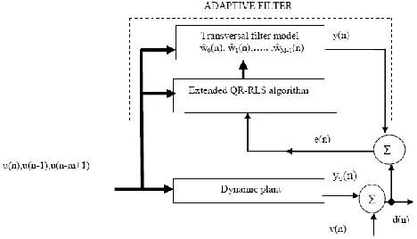
The adaptive filter could adjust with the characteristics of the input signal to maintain optimal filtering. While how to adjust the parameters is determined by the adaptive algorithm, the behavior of the adaptive algorithm is critical for the filtering performance. As is shown in Figure 1, the adaptive filter is consisted of the filter structure and the weight adjusting algorithm [8].

Fig. 1. The Schematic Model Diagram of Adaptive Filter

In most practical applications, where the second-order moments R(n) and d(n) are unknown, the use of an adaptive filter is the best solution. If the SOE (Signal Operating Environment) is ergodic, we have

N

H N

n N

1

R(n) lim u(n, )u (n, ) 2N 1

 _

  





(1)

*

1

d(n) lim u(n, )y (n, )

2 1



 





N N

n N

N   (2)

Here u n,

 

 is input signal, y n,

 

 is desired response signal

and N is the number of ensembles. The ensemble averages are equal to time averages. An adaptive filter consists of three key modules

1. An adjustable filtering structure that uses input samples to compute the output.

2. The criterion of performance that monitors the

performance of the filter.

3. The adaptive algorithm that updates the filter

coefficients.

The key component of any adaptive filter is the adaptive algorithm, which is a rule to determine the filter coefficients from the available data u n,

 

 andy n,

 

 . The dependence

of c n,

 

 on the input signal makes the adaptive filter a

recent update c n 1,



 



of the coefficient vector. The

adaptive filter, at each time n, performs the following computations:

 Filtering:

H

ˆy(n, )=c (n 1)x(n, )   (3)

 Error formation:

ˆ (n, )y(n, ) - y(n, )

e    (4)

 Adaptive algorithm:

  





   



c n, c n 1,   c x n, , e n, (5)

MSE use to measure the average of the squares of the errors. Error is the difference between the values implied by the estimator from the quantity to be estimated. MSE is the variance of the estimator so MSE has the same units of measurements as the square of the quantity being estimated.





n

2 i i i 1

1 _ˆ

MSE y y

n 





 (6)

Where ˆy_i is the vector of n predictions and y_iis the vector of

true values. The MSE of an estimator ˆ with respect of the unknown parameter is defined as

 

 

2

ˆ ˆ

MSE  E_    _

  (7)

A. Least Mean Square(LMS) adaptive filter algorithm

LMS algorithm update its weights to obtain optimal performance based on the least mean square criterion and gradient-descent methods. As LMS is an easy algorithm with less computation and simply implementing, as well as the robustness to statistical property of the signal, it is widely used in structural active vibration control area. LMS is linear adaptive filter algorithm and it is consisted of filtering process and adapting process [8].

 

  1

   

, 2 ,,

 



T k

w n w n w n w n

(8)

 

  1

   

, u2 ,

 



T k

u n u n n u n (9)

While the input signal is u n

 

, the tap weight vector isw n

 

. The output of the filter is

 

 T



1

  

y n w n u n (10)

The error function is

 



   



e n d n y n (11)

Mean-square error performance function

f w

 

is

 



 

2





f w E e n (12)

According to the least mean square criterion, the optimal filer

parameter w_opt should minimize the error performance

functionf w

 

. Using gradient-descent methods to

acquirew_opt, the weight update formula is

 





 1





,

   

,



w n w n f u n e n (13)

Here



is the convergence step factor and weight update function is

   





   

*

f u n , e n ,  e n u n (14)

Where



is the step-size factor and u(n) is the vector containing the L most recent samples of the system input signal. System output error is e(n), which is defined as:

 



 

ˆT

   

e n d n w n u n

(15)

where the corresponding filter output is:

 

 0

   



T

d n w u n v n (16)

Where v(n) is the system noise that is independent of the input signal u(n) and w0 is the optimal weight vector.

B. Normalized Least Mean Square(NLMS) adaptive filter algorithm

The main drawback of the “pure” LMS algorithm is that it is sensitive to the scaling of its input x(n). This makes it very hard (if not impossible) to choose a learning rate µ that guarantees stability of the algorithm [10]. The Normalized least mean squares filter (NLMS) is a variant of the LMS algorithm that solves this problem by normalizing with the power of the input.

H(0)=Zeros(p) (17)

InputSignalu n

 

_u n , u n 1 ,

  





u n



 p 1



_T (18)

For n=0,1,2,3,….

The error function is e n

 

d n

   

y n

(19)

 

 

H

   

e n d n h n u n (20)





 

H*

_{   }

   

e n u n h n 1 h n

U n U n



   (21)

the input u(n) and the real (unknown) impulse response h(n). In the general case with the interference (v n

 

0), the optimal learning rate is

   

 

2

opt 2

ˆ E y n y n

E e n

 _ 

 

 

 

 

(22)

C. Recursive Least Square(RLS) adaptive filter algorithm

Aiming to minimize the sum of the squares of the difference between the desired signal and the filter output, least square (LS) algorithm could use recursive form to solve least-squares at the moment the latest sampling value is acquired [6]. The filter output and the error function of RLS algorithm is

 

1 1H

_{  }



  

_{  }

P n 1 u n k n

1 u n P n 1 u n 



 



   (23)

Where k(n) is the gain vector, u(n) is the vector of buffered

input, p(n) is the inverse correlation matrix and



1denotes the reciprocal of the exponential weighting factor. The output of the filter is

 

 T



1

  

y n w n u n

(24)

Error signal e n

 

d n

   

y n (25)

The weighting update equation is

 





 1



H

   

w n w n k n e n (26)

 





 1



H

     

_  _

w n w n k n d n y n (27)

 





 1



H

   

_  T



1

  

_

w n w n k n d n w n x n (28)

Here

k

H

 

n

is the gain coefficient. With a sequence of training data up to time, the recursive least squares algorithm estimates the weight by minimizing the following cost [5]:

  







1 ₂

2

(n 1) 1

min ( ) 1  1







_    

n

T w

i

d i u i w n w n (29)

Where u(n) is the Lx1regressor input, d(n) is the desired response and λ is the regularization parameter.

D. Quadrative Recursive RLS (QR-RLS) adaptive filter algorithm

In the QR-RLS algorithm, or QR decomposition-based RLS algorithm, the computation of the least-squares weight vectors is accomplished by working directly with the incoming data matrix via the QR decomposition rather than working with the (time-averaged) correlation matrix of the input data as in the standard RLS algorithm in a finite-duration impulse response

filter implementation of the adaptive filtering algorithm Accordingly, the QR-RLS algorithm is numerically more stable than the standard RLS algorithm[7].

Fig. 2. System Identification for QR-RLS adaptive Filter

 



   

 



ˆu n  u 1 , u 2 ,, u n (30)

 



   

 



ˆd n  d 1 , d 2 ,, d n (31)

Here ˆu n

 

and ˆd n

 

are input signal vector and desired

response respectively. λ is taking as exponential weighting factor.

 

1/ 2

0 I

  



 0



(32)

P(0)=0 (33)

For n=1, 2 ………… compute









 

   

 

 

 

 

   

 

1/2 1/2 1/2

1/2 1/2 H 1/2

T H H/2 1/2

n 1 u n n 0

p n 1 d n n p n n n

0 1 u n  n n

      

   

     

   

   _{ } 

   

(34)

 

 

 

H H 1/ 2

ˆw n p n  n (35)

Computed 1/ 2

 

n

 & H

 

p n are the updated block values

andˆw n

 

is the least-squares weight vector.

III.

S

IMULATION ANALYSIS

0 100 200 300 400 500 600 700 800 -14

-12 -10 -8 -6 -4 -2 0 2 4 6

Learning behavior curve for MSE using LMS Algorithm

Number of iterations, k

M

S

E

[

d

B

]

Figure 3. MSE Curve for LMS Algorithm

0 100 200 300 400 500 600 700 800

-15 -10 -5 0 5 10

Learning behavior Curve for MSE using NLMS Algorithm

Number of iterations, k

M

S

E

[

d

B

]

Fig. 4. MSE Curve for NLMS Algorithm

0 100 200 300 400 500 600 700 800 -14

-12 -10 -8 -6 -4 -2 0 2

Learning behavior Curve for MSE using RLS Algorithm

Number of iterations, k

M

S

E

[

d

B

]

Fig. 5. MSE Curve for RLS Algorithm

0 100 200 300 400 500 600 700 800 -20

-15 -10 -5 0 5 10

Number of iterations, k

M

S

E

[

d

B

]

Learning Curve for MSE

LMS NLMS RLS

Fig. 6. Comparison of MSE Curve for LMS, NLMS & RLS Algorithm

0 100 200 300 400 500 600 700 800

-26 -25 -24 -23 -22 -21 -20 -19 -18 -17

Learning behavior Curve for MSE using QR-RLS Algorithm

Number of iterations, k

M

S

E

[

d

B

]

Fig. 7. MSE Curve for QR-RLS Algorithm

0 100 200 300 400 500 600 700 800 -25

-20 -15 -10 -5 0 5 10

Number of iterations, k

M

S

E

[

d

B

]

Learning Curve for MSE

LMS NLMS RLS QR-RLS

Fig. 8. Comparison of MSE Curve for LMS, NLMS, RLS & QR-RLS Algorithm

RLS algorithm respectively. Figure 6 displaying the comparison between all these three algorithms. Figure 7 shows the MSE curve of QR-RLS algorithm and Figure 8 shows the final comparison curve between MSE of LMS, NLMS and RLS with QR-RLS algorithm.

IV.

SIMULATION RESULTS

Simulation of LMS, NLMS, RLS & QR-RLS adaptive filter algorithm with the signal x. In this x is chosen according to the 4-QAM constellation. The variation of x is normalized to 1. The complex MSK data is generated for 100 ensembles. From the plots it is clear that the RLS achieve faster initial convergence speed than LMS and NLMS and in the comparison of MSE, QR-RLS has lowest MSE_av (db) with compare to other algorithms. RLS algorithms (RLS & QR-RLS) although converges faster but it is computationally more complex as matrix inversion is involved. In order to compare these algorithms easily, the best parameters in above simulation results are selected. In Figure 8, µ=0.2 for LMS adaptive filters (LMS & NLMS) and λ=0.8 for RLS adaptive filters (RLS & QR-RLS) is set for their best MSE performance.

V.

CONCLUSION

In this paper an advance algorithm for identify an unknown FIR filter system has been presented to enhance the performance and improve the convergence property of the previously proposed adaptive methods. A comparison between the MSE performance of LMS, NLMS, RLS and QR-RLS algorithm have been shown. All results show that the RLS algorithm outperforms the LMS & NLMS algorithm in terms of convergence rate and the learning behavior. In terms of MSE the QR-RLS gives better performance than other filter identification algorithms.

REFERENCES

[1] Udawat, A. , Sharma, P.C. ; Katiyal, S., “Performance analysis and comparison of adaptive beam forming algorithms for Smart Antenna Systems”, Next Generation Networks, 2010 International Conference, p.p. 1 – 5, Sept. 2010

[2] Djigan, V.I. , “Adaptive filtering algorithms with quatratized cost function for Linearly Constrained arrays”, Antenna Theory and Techniques (ICATT), 2013 IX International Conference, p.p. 214 – 216, Sep. 2013

[3] Soumya, R.G., Naveen, N., Lal, M.J., “Application of

Adaptive Filter Using Adaptive Line Enhancer

Techniques” Advances in Computing and

Communications (ICACC), 2013 Third International Conference, p.p. 165 – 168, Aug. 2013

[4] Yu Xia “Performance analysis of adaptive filters for time-varying systems”, Control Conference (CCC), 2013 32nd Chinese, p.p. 8572 – 8575, July 2013

[5] Huang, Y.J. Wang, Y.W. ; Meng, F.J. ; Wang, G.L., “A spatial spectrum estimation algorithm based on adaptive beam forming nulling” Intelligent Control and Information

Processing (ICICIP), 2013 Fourth International

Conference, p.p. 220 – 224, June 2013

[6] Salman, M.S. , Yilmaz, M.F., “Adaptive filtering for incident plane wave estimation” Technological Advances in Electrical, Electronics and Computer Engineering (TAEECE), 2013 International Conference, p.p. 162 – 165, May 2013.

[7] J. Mehena, L. Swain, G. Patnaik, “System Identification based on QR- Decomposition” Int. J. of Intelligent Computing and Applied Sciences, p.p.31-39, ISSN: 2322-0031, Vol. 1, Issue1 2013.

[8] Huang Quanzhen, Gao Zhiyuan, Gao Shouwei, Shao

Yong, Zhu Xiaojin, “Comparison of LMS and RLS Algorithm for active vibration control of smart structures” 3rd International Conference on Measuring Technology and Mechatronics Automation, IEEE , pp. 745-748, 2011

[9] Lei Wang, Rodrigo C. de Lamare, “Constrained Constant

Modulus RLS-based Blind Adaptive Beamforming

Algorithm for Smart Antennas”, Wireless Communication Systems (ISWCS 2007) 4th International Symposium, p.p. 657 – 661, Oct. 2007

[10]S. Haykin, Adaptive Filter Theory. Prentice Hall, Inc., 1996.

[11]S. Haykin, Modern Filters. Maxwell Macmillan