Atmos. Meas. Tech., 11, 2863–2878, 2018 https://doi.org/10.5194/amt-11-2863-2018 © Author(s) 2018. This work is distributed under the Creative Commons Attribution 4.0 License.
Preliminary verification for application of a support vector
machine-based cloud detection method to GOSAT-2 CAI-2
Yu Oishi1,a, Haruma Ishida2, Takashi Y. Nakajima3, Ryosuke Nakamura1, and Tsuneo Matsunaga4 1National Institute of Advanced Industrial Science and Technology, 2-4-7 Aomi, Koto, Tokyo 135-0064, Japan 2Meteorological Research Institute, 1-1 Nagamine, Tsukuba, Ibaraki 305-0052, Japan
3Research and Information Center, Tokai University, 2-28-4 Tomigaya, Shibuya, Tokyo 151-0063, Japan 4National Institute for Environmental Studies, 16-2 Onogawa, Tsukuba, Ibaraki 305-8506, Japan
acurrently at: National Agriculture and Food Research Organization, 3-1-1 Kannondai, Tsukuba, Ibaraki 305-8517, Japan Correspondence:Yu Oishi ([email protected])
Received: 18 December 2017 – Discussion started: 22 January 2018
Revised: 25 April 2018 – Accepted: 29 April 2018 – Published: 17 May 2018
Abstract. The Greenhouse Gases Observing Satel-lite (GOSAT) was launched in 2009 to measure global atmospheric CO2 and CH4 concentrations. GOSAT is equipped with two sensors: the Thermal And Near infrared Sensor for carbon Observations (TANSO)-Fourier trans-form spectrometer (FTS) and TANSO-Cloud and Aerosol Imager (CAI). The presence of clouds in the instantaneous field of view of the FTS leads to incorrect estimates of the concentrations. Thus, the FTS data suspected to have cloud contamination must be identified by a CAI cloud discrimi-nation algorithm and rejected. Conversely, overestimating clouds reduces the amount of FTS data that can be used to estimate greenhouse gas concentrations. This is a serious problem in tropical rainforest regions, such as the Amazon, where the amount of useable FTS data is small because of cloud cover. Preparations are continuing for the launch of the GOSAT-2 in fiscal year 2018. To improve the accuracy of the estimates of greenhouse gases concentrations, we need to refine the existing CAI cloud discrimination algo-rithm: Cloud and Aerosol Unbiased Decision Intellectual Algorithm (CLAUDIA1). A new cloud discrimination algorithm using a support vector machine (CLAUDIA3) was developed and presented in another paper. Although the use of visual inspection of clouds as a standard for judging is not practical for screening a full satellite data set, it has the advantage of allowing for locally optimized thresholds, while CLAUDIA1 and -3 use common global thresholds. Thus, the accuracy of visual inspection is better than that of these algorithms in most regions, with the exception of
snow- and ice-covered surfaces, where there is not enough spectral contrast to identify cloud. In other words, visual inspection results can be used as truth data for accuracy evaluation of CLAUDIA1 and -3. For this reason visual inspection can be used for the truth metric for the cloud dis-crimination verification exercise. In this study, we compared CLAUDIA1–CAI and CLAUDIA3–CAI for various land cover types, and evaluated the accuracy of CLAUDIA3–CAI by comparing both CLAUDIA1–CAI and CLAUDIA3–CAI with visual inspection (400×400 pixels) of the same CAI images in tropical rainforests. Comparative results between CLAUDIA1–CAI and CLAUDIA3–CAI for various land cover types indicated that CLAUDIA3–CAI had a tendency to identify bright surface and optically thin clouds. However, CLAUDIA3–CAI had a tendency to misjudge the edges of clouds compared with CLAUDIA1–CAI. The accuracy of CLAUDIA3–CAI was approximately 89.5 % in tropical rainforests, which is greater than that of CLAUDIA1–CAI (85.9 %) for the test cases presented here.
1 Introduction
green-Figure 1.Monthly changes in the number of FTS L2 XCO2data in the Amazon. The five-point cross-track scan mode was used until 1 August 2010, when it was replaced with the three-point cross-track scan mode. Therefore the numbers themselves before and after 1 August 2010 cannot be compared.
house gases performed by GOSAT, to monitor the effects of climate change and human activities on the carbon cycle, and to contribute to climate science and climate change re-lated policies (NIES GOSAT-2 Project, 2014). These poli-cies include Reducing Emissions from Deforestation and Forest Degradation and the role of conservation; sustain-able management of forests and enhancement of forest car-bon stocks in developing countries (REDD+); and the Joint Crediting Mechanism (JCM), which was proposed by the Japanese government to facilitate the diffusion of leading low-carbon technologies, products, systems, services, and infrastructure in developing countries (Ministry of the En-vironment, Japan, 2015). Monthly regional CO2 fluxes are estimated from the column-averaged dry-air mole fractions of CO2 (XCO2)retrieved from spectral observations made by GOSAT (Maksyutov et al., 2013). The results are pub-licly available as the L4A CO2 product (Maksyutov et al., 2014). The expected role of the CO2fluxes estimated from the GOSAT data is the system for measurement, reporting and verification (MRV) of CO2fluxes estimated from forest inventory data. Currently, the uncertainty of the L4A CO2 product is about 0.9 Gt-C region−1yr−1in the Amazon (L4A CO2product V02.03 in region ln 09-12, 2009–2012). Thus, the total net CO2flux from deforestation for the period 2000– 2010 in tropical America was estimated to be 0.56 Gt-C yr−1 (Baccini et al., 2012). It is required to reduce the uncertainty of the L4A CO2product by a factor of 16, assuming that the MRV for REDD+and JCM needs an accuracy of 10 %.
GOSAT is equipped with two sensors: the Thermal And Near infrared Sensor for carbon Observations (TANSO)-Fourier transform spectrometer (FTS) and TANSO-Cloud and Aerosol Imager (CAI) (Table 1). The presence of clouds in the instantaneous field of view of the FTS leads to
incor-Figure 2. Clear-sky probability at 0.1◦×0.1◦ calculated with MYD35_L2. There are low clear-sky probabilities over most tropi-cal rainforests because the moisture helps to create clouds.
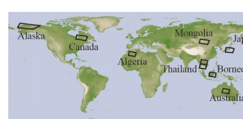
Figure 3.Study areas for various land cover types. Black rectangles indicate the locations of CAI frames.
prod-Y. Oishi et al.: Preliminary verification for application of a support vector machine 2865
Table 1.Specifications of CAI.
Band 1 Band 2 Band 3 Band 4
Spectral coverage NUV Red NIR SWIR
(µm) 0.370–0.390 0.664–0.684 0.860–0.880 1.56–1.65
Swath (km) 1000 1000 1000 750
Spatial resolution 500 500 500 1500
At nadir (m)
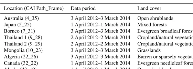
Table 2.GOSAT CAI L1B product and CAI L2 cloud flag product used for various land cover types in this study. Land cover was derived from the MODIS land cover type product (MCD12). Japan scenes include urban areas.
Location (CAI Path_Frame) Data period Land cover
Australia (4_35) 3 April 2012–3 March 2014 Open shrublands Japan (5_25) 1 April 2012–1 March 2014 Mixed forests
Borneo (7_31) 3 April 2012–3 March 2014 Evergreen broadleaf forest Thailand 1 (9_28) 2 April 2012–2 March 2014 Cropland/natural vegetation Thailand 2 (9_29) 2 April 2012–2 March 2014 Cropland/natural vegetation Mongolia (10_23) 3 April 2012–3 March 2014 Grasslands
Algeria (22_26) 3 April 2012–3 March 2014 Barren or sparsely vegetated Canada (32_22) 1 April 2012–1 March 2014 Evergreen needleleaf forest Alaska (43_19) 1 April 2012–1 March 2014 Open shrublands
Figure 4.Study areas in Borneo and the Amazon. CAI path and frame system: XX_YY (XX indicates CAI path number and YY indicates CAI frame number). Red rectangles indicate the locations of CAI frames. The background image was generated from the CAI L3 global reflectance distribution product (15 June to 14 July 2013).
uct may not be sensitive enough to detect clouds of subpixel size in ocean observations. To cope with these difficulties, the FTS data suspected to have cloud contamination are identi-fied by two additional tests: the 2 µm band test and the CAI coherent test (Yoshida et al., 2010). Conversely, overestima-tion of clouds reduces the amount of the FTS data that can be used to estimate greenhouse gas concentrations. This is a serious problem in tropical rainforest regions, such as the Amazon, where there is a small amount of suitable FTS data (approximately 3 % of the number of observations) because of cloud cover (Figs. 1 and 2). For this reason we need to
optimize thresholds between cloudy and clear sky because there are tradeoffs in maximizing cloud detection accuracy while minimizing false detection. To solve the problem, a new cloud discrimination algorithm (CLAUDIA3) using a support vector machine (SVM) (Vapnik and Lerner, 1963) was developed (Ishida et al., 2018). CLAUDIA3 can auto-matically identify the optimized thresholds using clear-sky training data, although CLAUDIA1 requires setting various thresholds by radiative transfer calculation results and fine tuning in some methods. Verification was also performed by comparing it with the MODIS cloud mask algorithm (Ack-erman et al., 2010) and ceilometer data provided by the At-mospheric Radiation Measurement Climate Research Facil-ity (Mather and Voyles, 2013) in Ishida et al. (2018). Further-more the impact of different support vector generation pro-cedures on cloud discrimination using CLAUDIA3 has also been evaluated in a previous study (Oishi et al., 2017).
Table 3.GOSAT CAI L1B product and CAI L2 cloud flag product used for rainforests in this study.
Borneo Amazon
Date Location Date Location
(yy/mm/dd) (CAI Path_Frame) (yy/mm/dd) (CAI Path_Frame)
10/04/02 7_30 11/08/28 28_31
10/01/02 7_31 11/08/28 28_32
10/04/02 7_31 11/08/28 28_33
10/07/01 7_31 11/08/29 29_31
10/07/07 7_31 10/08/28 29_32
10/07/13 7_31 11/02/03 29_32
10/07/19 7_31 11/04/01 29_32
10/07/28 7_31 11/06/03 29_32
10/09/02 7_31 11/08/02 29_32
10/11/01 7_31 11/08/08 29_32
11/08/14 29_32
11/08/23 29_32
11/08/29 29_32
11/10/01 29_32
11/12/03 29_32
11/08/29 29_33
11/08/30 30_31
11/08/30 30_32
11/08/30 30_33
CLAUDIA1 and -3 use common global thresholds. Thus, the accuracy of visual inspection is better than that of these algo-rithms in most regions, with the exception of snow- and ice-covered surfaces, where there is not enough spectral contrast to distinguish cloud. In other words, visual inspection results can be used as truth data for accuracy evaluation of CLAU-DIA1 and -3. For this reason visual inspection can be used as the truth metric for the verification exercise. Therefore, the accuracy of CLAUDIA1–CAI has also been evaluated by vi-sual inspection in tropical rainforests (Oishi et al., 2014). In this study, we deal with the application of the CLAUDIA3 to GOSAT CAI data. Then, we compare CLAUDIA1–CAI and CLAUDIA3–CAI for various land cover types and evaluate their accuracy by comparing both against visual inspection (400×400 pixels) of the same CAI images in tropical rain-forests.
2 Materials and methods 2.1 Study area and data
The study area for directly comparing CLAUDIA1–CAI and CLAUDIA3–CAI for various land cover types is the same as in the previous study (Oishi et al., 2017) (Fig. 3) and the accuracy can be evaluated by comparing them against visual inspection in Borneo and the Amazon (Fig. 4).
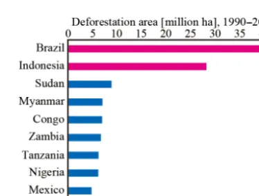
The total forest area in the Amazon, Congo, and south-east Asia rainforest basins is over 13 million km2, which corre-sponds to one-third of the total global forest area (FAO and
Figure 5.List of the top 10 countries for changes in deforesta-tion area (million ha) from 1990 to 2005. These were calculated with data from the Global Forest Resources Assessment 2005 (FAO, 2005).
Y. Oishi et al.: Preliminary verification for application of a support vector machine 2867
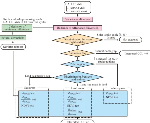
Figure 6.Flow chart for CLAUDIA1–CAI. For sun-glint areas, the thresholds are further increased based on theR0.87 µmtest. CCL is confidence level,Rwavelengthis reflectance, NDVI is normalized difference vegetation index.
GOSAT returns to a similar footprint after 44 orbits (44 CAI paths) in 3 days. The satellite ground path of one or-bit is divided into 60 equidistant CAI frames. We used the GOSAT CAI L1B product, which general users could down-load from the GOSAT User Interface Gateway (GUIG, https: //data.gosat.nies.go.jp), for various land cover types at the be-ginning of the month from 2012 to 2014 as was done in the previous study (Oishi et al., 2017) (Table 2), and for rain-forests (Table 3). Recently the GUIG has been changed to GOSAT Data Archive Service (GDAS, https://data2.gosat. nies.go.jp/index_en.html). The spatial resolution of these products (pixel size at nadir) is 500 m, and the image size is 2048×1355 pixels (approximately 1000×680 km). The CLAUDIA algorithm requires a land–sea mask and surface albedo data. The CAI L1B product includes a land–sea mask with 500 m resolution, which is generated from the Shut-tle Radar Topography Mission’s 15? land–sea mask and the
USGS Global Land 1-km AVHRR Data Set Project mask for areas at latitudes higher than±60◦. Surface albedo data at 1/30◦resolution was generated from the CAI L1B data from 10 recurrent cycles by separating the land and water regions. This processing consists of three steps (Ishihara and Nobuta, 2013):
1. calculate the minimum reflectance to remove cloud-contaminated pixels,
2. cloud shadow correction (Fukuda et al., 2013), and 3. atmospheric correction.
2.2 CLAUDIA1
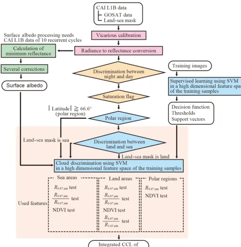
Figure 7.Flow chart for CLAUDIA3–CAI. CCL is clear-sky confidence level, Rwavelength is reflectance, NDVI is normalized difference vegetation index.
integration (Ishida and Nakajima, 2009). Integrated CCL of 0 means that the pixel is cloudy and 1 means that the pixel is cloud-free. Ambiguous pixels between cloudy and cloud-free are described by numerical values from 0 to 1. The threshold below which the integrated CCL counts the pixel as cloud-free for GOSAT FTS L2 is 0.33, otherwise the pixel is re-garded as cloudy (Yoshida et al., 2010). The flow of the al-gorithm is shown in Fig. 6.
2.3 New cloud discrimination algorithm (CLAUDIA3)
Y. Oishi et al.: Preliminary verification for application of a support vector machine 2869
Figure 8.Analysis procedure.(a)CAI L1B image.(b)Visual inspection mask of CAI L1B.(c)Output mask from CLAUDIA1–CAI (CAI L2 cloud flag product) or CLAUDIA3–CAI. Pixels that are determined as cloudy are black.(d)Comparison of the visual inspection image and the output image. Pixels that are determined as cloudy in both are white. Pixels that are determined as clear in both are blue. Pixels that are determined as cloudy in the output image and clear in the visual inspection image are green. Unusual pixels that are determined as clear in the output image and cloudy in the visual inspection image are red.
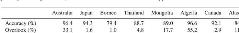
Table 4.Yearly average accuracy, overlook, and overestimate for various land cover types.
Australia Japan Borneo Thailand Mongolia Algeria Canada Alaska
Accuracy (%) 96.4 94.3 79.4 88.7 89.0 96.6 92.1 84.2
Overlook (%) 33.1 1.6 1.0 4.8 17.7 55.2 2.9 11.9
Overestimate (%) 0.1 13.7 39.2 20.9 11.7 0.7 51.8 50.3
discriminate between two classifications (clear and cloudy), (2) the thresholds, and (3) the support vectors, which are training samples specified by the decision function. The sup-port vectors are decided in a high-dimensional feature space of the training samples. Next, it performs cloud discrimina-tion by using the decision funcdiscrimina-tion, thresholds, and support vectors it determined. CLAUDIA3 applies the kernel trick (Boser et al., 1992) for soft-margin SVM (Cortes and Vapnik, 1995). The kernel uses a second-order polynomial (Eq. 1).
K(xi,x)=(xiqx+1)
2
2 , (1)
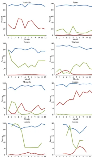
Figure 9.Monthly average accuracy, overlook, and overestimate for various land cover types. Blue line indicates accuracy, red line indicates overlook, and green line indicates overestimate.
2.4 Analysis procedure for rainforests
The analysis procedure consists of the following steps (Fig. 8).
1. Cut 400×400 pixels around the center of CAI L1B im-ages.
2. Perform a visual inspection of the pixels cut from the CAI L1B images.
We performed a visual inspection of the presence or ab-sence of clouds in every pixel (400×400 pixels). 3. Perform cloud discrimination by using CLAUDIA1–
Y. Oishi et al.: Preliminary verification for application of a support vector machine 2871
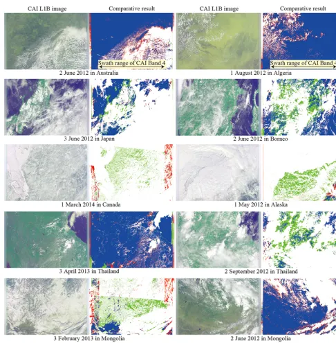
Figure 10.CAI L1B images (R: Band 2, G: Band 3, B: Band 1) and comparative results of CLAUDIA1–CAI and CLAUDIA3–CAI for various land cover types.
For CLAUDIA1–CAI, we produced output images setting the integrated-CCL threshold to 0.33. For CLAUDIA3–CAI, we produced output images setting the integrated-CCL threshold to 0.5.
4. Compare output with visual inspection.
We colored the images by comparing the visual inspec-tion images with the output images pixel by pixel.
3 Results
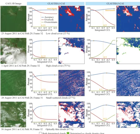
Figure 11.Comparison of the visual inspection images and the output images in the Amazon. Orange circles indicate the maximum accuracy values. Orange dotted lines indicate the integrated-CCL thresholds. Blue line indicates the accuracy, red line indicates the overlook, and green line indicates the overestimate.
were judged cloudy in the standard image. “Overestimate” is defined as the ratio of the number of pixels judged cloudy in the output and clear in the standard image to the number of pixels judged clear in the standard image. These definitions are written as follows.
Accuracy=Both cloudy+Both clear
Total number of pixels , (2)
Overlook= Clear despite cloudy
Both cloudy+clear despite cloudy, (3) Overestimate= Cloudy despite clear
Both clear+cloudy despite clear. (4) 3.1 Results for various land cover types
overesti-Y. Oishi et al.: Preliminary verification for application of a support vector machine 2873
Table 5.Results for integrated-CCL thresholds of 0.33 for CLAUDIA1–CAI and 0.5 for CLAUDIA3–CAI in the Amazon.
Accuracy (%) Overlook (%) Overestimate (%)
Date Location CLAUDIA1 CLAUDIA3 CLAUDIA1 CLAUDIA3 CLAUDIA1 CLAUDIA3 (0.5)
(yy/mm/dd) (CAI Path_Frame) (0.33) (0.5) (0.33) (0.5) (0.33) (0.5)
11/08/28 28_31 84.6 95.1 56.6 16.9 0.0 0.5
11/08/28 28_32 80.6 92.9 49.7 7.5 0.1 6.9
11/08/28 28_33 92.0 95.9 11.6 13.4 7.4 2.4
11/08/29 29_31 87.6 93.8 27.2 9.5 0.3 3.5
10/08/28 29_32 89.8 90.8 32.6 9.9 1.7 9.0
11/02/03 29_32 86.6 92.9 35.5 2.4 0.5 9.9
11/04/01 29_32 95.0 91.6 5.8 0.1 2.1 36.6
11/06/03 29_32 89.9 90.2 38.1 4.1 0.8 11.7
11/08/02 29_32 77.9 90.6 71.0 27.3 0.1 1.5
11/08/08 29_32 84.5 92.9 66.0 26.3 0.1 1.2
11/08/14 29_32 87.8 93.2 77.4 36.0 0.1 1.4
11/08/23 29_32 90.0 92.2 77.8 54.0 0.1 1.0
11/08/29 29_32 79.6 91.0 52.4 19.7 0.1 2.2
11/10/01 29_32 87.1 92.2 33.9 5.5 0.1 9.1
11/12/03 29_32 82.8 93.4 30.7 1.7 0.1 12.9
11/08/29 29_33 90.6 90.8 20.8 15.1 2.3 5.6
11/08/30 30_31 85.7 85.1 24.7 9.2 3.2 21.0
11/08/30 30_32 86.0 91.4 20.9 10.2 0.4 5.5
11/08/30 30_33 94.9 93.0 11.1 3.6 1.5 9.1
Average 87.0 92.0 39.1 14.3 1.1 7.9
Table 6.Results for integrated-CCL thresholds of the maximum accuracy values in Fig. 11 (CLAUDIA1–CAI: 0.75, CLAUDIA3–CAI: 0.5) in the Amazon.
Accuracy (%) Overlook (%) Overestimate (%)
Date Location CLAUDIA1 CLAUDIA3 CLAUDIA1 CLAUDIA3 CLAUDIA1 CLAUDIA3
(yy/mm/dd) (CAI Path_Frame) (0.75) (0.5) (0.75) (0.5) (0.75) (0.5)
11/08/28 28_31 86.9 95.1 47.9 16.9 0.0 0.5
11/08/28 28_32 84.2 92.9 40.2 7.5 0.2 6.9
11/08/28 28_33 83.6 95.9 7.1 13.4 18.1 2.4
11/08/29 29_31 89.6 93.8 21.8 9.5 1.2 3.5
10/08/28 29_32 90.6 90.8 23.5 9.9 4.0 9.0
11/02/03 29_32 88.9 92.9 27.8 2.4 1.4 9.9
11/04/01 29_32 96.2 91.6 3.7 0.1 4.1 36.6
11/06/03 29_32 90.9 90.2 29.3 4.1 2.4 11.7
11/08/02 29_32 80.1 90.6 63.6 27.3 0.3 1.5
11/08/08 29_32 85.9 92.9 59.4 26.3 0.2 1.2
11/08/14 29_32 88.8 93.2 70.1 36.0 0.2 1.4
11/08/23 29_32 90.9 92.2 70.3 54.0 0.1 1.0
11/08/29 29_32 82.2 91.0 45.5 19.7 0.2 2.2
11/10/01 29_32 89.7 92.2 26.6 5.5 0.4 9.1
11/12/03 29_32 86.7 93.4 23.3 1.7 0.5 12.9
11/08/29 29_33 90.9 90.8 13.5 15.1 6.4 5.6
11/08/30 30_31 87.1 85.1 20.4 9.2 4.9 21.0
11/08/30 30_32 89.9 91.4 14.7 10.2 1.0 5.5
11/08/30 30_33 95.1 93.0 7.0 3.6 3.6 9.1
Table 7.Results for integrated-CCL thresholds of 0.33 for CLAUDIA1–CAI and 0.5 for CLAUDIA3–CAI in Borneo.
Accuracy (%) Overlook (%) Overestimate (%)
Date Location CLAUDIA1 CLAUDIA3 CLAUDIA1 CLAUDIA3 CLAUDIA1 CLAUDIA3
(yy/mm/dd) (CAI Path_Frame) (0.33) (0.5) (0.33) (0.5) (0.33) (0.5)
10/04/02 7_30 89.7 91.7 28.8 1.7 0.1 12.0
10/01/02 7_31 85.6 85.0 25.8 1.8 0.6 31.1
10/04/02 7_31 94.8 85.4 8.3 0.6 3.5 22.8
10/07/01 7_31 90.8 92.2 29.0 5.0 0.4 9.0
10/07/07 7_31 76.5 85.9 54.2 22.5 0.5 7.8
10/07/13 7_31 88.2 89.1 32.6 5.8 2.0 13.3
10/07/19 7_31 77.1 88.4 31.1 11.0 1.0 13.5
10/07/28 7_31 70.6 81.5 44.8 8.2 1.1 37.5
10/09/02 7_31 89.3 87.8 37.8 6.5 1.3 14.2
10/11/01 7_31 85.8 81.8 20.6 0.4 1.2 54.7
Average 84.8 86.9 31.3 6.3 1.2 21.6
Table 8. Results for integrated-CCL thresholds of the maximum accuracy values in Fig. 13 (CLAUDIA1–CAI: 0.85, CLAUDIA3–CAI: 0.35) in Borneo.
Accuracy (%) Overlook (%) Overestimate (%)
Date Location CLAUDIA1 CLAUDIA3 CLAUDIA1 CLAUDIA3 CLAUDIA1 CLAUDIA3
(yy/mm/dd) (CAI Path_Frame) (0.85) (0.35) (0.85) (0.35) (0.85) (0.35)
10/04/02 7_30 91.9 94.6 22.3 8.5 0.3 3.8
10/01/02 7_31 89.2 90.7 16.8 8.0 3.6 10.9
10/04/02 7_31 93.8 91.5 4.6 2.3 7.2 12.2
10/07/01 7_31 92.1 93.2 21.5 10.3 1.9 5.3
10/07/07 7_31 79.4 83.5 46.1 33.0 1.6 4.2
10/07/13 7_31 88.9 90.9 25.1 11.4 4.4 7.9
10/07/19 7_31 81.7 83.4 24.1 20.1 2.7 7.1
10/07/28 7_31 77.3 80.7 33.2 18.9 3.2 20.0
10/09/02 7_31 90.3 90.6 29.0 12.3 3.0 8.3
10/11/01 7_31 90.8 89.4 10.9 3.3 5.8 25.5
Average 87.5 88.8 23.4 12.8 3.4 10.5
Figure 12. Average accuracy, overlook, and overestimate for all data for the Amazon. The most suitable integrated-CCL thresholds are 0.75 for CLAUDIA1–CAI and 0.5 for CLAUDIA3–CAI in the Amazon.
mate. We used the CLAUDIA1–CAI result as the standard image.
Y. Oishi et al.: Preliminary verification for application of a support vector machine 2875
Figure 13.Figure 13 compares the results of the visual inspection images and the output images for two select cases in Borneo: small scattered clouds and optically thin clouds. We used the visual inspection result as the standard image. The comparison of the results for Borneo is similar to that for the Amazon. Figure 14 shows the average accuracy, overlook, and overestimate of all data for all cases in Borneo. These results indicate that the most suitable integrated-CCL thresholds are 0.85 for the CLAUDIA1–CAI and 0.35 for CLAUDIA3– CAI in Borneo. Since the curved lines of the overestimate and overlook intersect in the same way as the Amazon cases, CLAUDIA3–CAI can appropriately determine the boundary between cloudy and clear sky.
Figure 14.Comparison of the visual inspection images and the out-put images in Borneo. Orange circles indicate the maximum accu-racy values. Orange dotted lines indicate the integrated-CCL thresh-olds. Blue line indicates the accuracy, red line indicates the over-look, and green line indicates the overestimate.
Figure 10 compares the output images of CLAUDIA1– CAI and CLAUDIA3–CAI for select cases in each region.
In Australia and Algeria, CLAUDIA3–CAI could identify bright surfaces; however, there were a few oversights at the edges of clouds. In Japan, CLAUDIA3–CAI misjudged veg-etation areas as clouds. In Borneo, CLAUDIA3–CAI could identify optically thin clouds. In Canada and Alaska, they were snow- or ice-covered scenes. Since the CAI is not equipped with any thermal infrared bands, cloud discrimi-nation based on the temperature at the top of clouds is not
feasible. Accordingly, it is difficult to discriminate between ice or snow and clouds. The difference or similarity between CLAUDIA1–CAI and CLAUDIA3–CAI was attributed to this source of error. In Thailand, CLAUDIA3–CAI could judge smoke as noncloud, despite CLAUDIA1–CAI mis-judging smoke as cloud; however, there were oversights of optically thin clouds and the edges of clouds on 3 April 2013. Furthermore CLAUDIA3–CAI misjudged muddy rivers and boundaries between land and water as cloudy. This was also reported for CLAUDIA1–CAI in a previous study (Oishi et al., 2014). Conversely, CLAUDIA3–CAI could identify op-tically thin clouds on 2 September 2012. In Mongolia, there was a snow-covered scene on 3 February 2013 and the same as Canada and Alaska. On the other hand CLAUDIA3–CAI could identify bright surface; however, there were a few over-sights at the edges of clouds on 2 June 2012.
3.2 Results in the Amazon
Figure 11 compares the visual inspection images and the out-put images for four select cases in the Amazon: low cloud cover, high cloud cover, small scattered clouds, and optically thin clouds. We used the visual inspection result as the stan-dard image.
occur at different integrated-CCL values with the thresholds for the Amazon. Figure 12 shows the average accuracy, over-look, and overestimate of all the data in the Amazon for all 19 cases. These results indicate that the most suitable integrated-CCL thresholds are 0.75 for CLAUDIA1–CAI and 0.5 for CLAUDIA3–CAI in the Amazon. Since the curved lines of the overestimate and overlook intersect, CLAUDIA3–CAI can appropriately determine the boundary between cloudy and clear sky.
Table 5 shows the results for an integrated-CCL thresh-old of 0.33 for CLAUDIA1–CAI and 0.5 for CLAUDIA3– CAI, and Table 6 shows the results for an integrated-CCL threshold of the maximum accuracy values in Fig. 12 (CLAUDIA1–CAI: 0.75, CLAUDIA3–CAI: 0.5). There was no notable change in the accuracies with the season or lo-cation. When the integrated-CCL threshold was 0.33 for CLAUDIA1–CAI and 0.5 for CLAUDIA3–CAI, the accura-cies were 87.0 and 92.0 %, respectively. When the accuracy of CLAUDIA1–CAI was higher than that of CLAUDIA3– CAI, optically thick clouds covered a large area of the in-put images. Furthermore, when the integrated-CCL thresh-old was 0.75 for CLAUDIA1–CAI and 0.5 for CLAUDIA3– CAI, the accuracies were at their highest, at 88.3 and 92.0 %, respectively. In both cases, the accuracy of CLAUDIA3–CAI was higher than that of CLAUDIA1–CAI.
3.3 Results in Borneo
Average accuracy, overlook, and overestimate for all data for Borneo. The most suitable integrated-CCL thresholds are 0.85 for CLAUDIA1–CAI and 0.35 for CLAUDIA3–CAI in Borneo.
Table 7 shows the results for an integrated-CCL thresh-old of 0.33 for CLAUDIA1–CAI and 0.5 for CLAUDIA3– CAI, and Table 8 shows the results for an integrated-CCL threshold of the maximum accuracy values in Fig. 14 (CLAUDIA1–CAI: 0.85, CLAUDIA3–CAI: 0.35). There was no notable change in the accuracies with the sea-son or location, similar to the results for the Amazon. For an integrated-CCL threshold of 0.33 for CLAUDIA1–CAI and 0.5 for CLAUDIA3–CAI, the accuracies were 84.8 and 86.9 %, respectively. Furthermore, for an integrated-CCL threshold of 0.85 for CLAUDIA1–CAI and 0.35 for CLAUDIA3–CAI, the highest accuracies of 87.5 and 88.8 %, respectively, were obtained. In both cases, the accuracy of CLAUDIA3–CAI was greater than that of CLAUDIA1–CAI.
4 Discussions and conclusions
Comparative results for CLAUDIA1–CAI and CLAUDIA3– CAI for various land cover types indicated that CLAUDIA3– CAI had a tendency to identify bright surface and optically thin clouds; however, CLAUDIA3–CAI had a tendency to misjudge the edges of clouds compared with CLAUDIA1–
CAI. There are tradeoffs in maximizing accuracy while min-imizing overlook and overestimate. Thus, it is sufficient to change the integrated-CCL threshold according to the pur-pose. Furthermore, CLAUDIA3–CAI misjudged vegetation areas as clouds in Japan. It is necessary to add clear training data of Japanese vegetation areas for CLAUDIA3.
The averaged accuracy of CLAUDIA3 used with GOSAT CAI data (CLAUDIA3–CAI) was approximately 89.5 % in tropical rainforests, which was greater than that of CLAUDIA1–CAI (85.9 %) for the test cases presented here. This is mainly because, in contrast to CLAUDIA1–CAI, CLAUDIA3–CAI can detect optically thin clouds and the edges of clouds, which prevents cloud-contaminated FTS-2 data from being processed as cloud-free FTS-FTS-2 data in the greenhouse gas concentration calculations. However, CLAUDIA3–CAI tends to overestimate the surroundings of clouds, which are judged to be cloudy despite being clear. Thus, CLAUDIA3–CAI is not expected to increase the amount of the FTS-2 data that can be used to estimate green-house gas concentrations in tropical rainforests. Conversely, CLAUDIA3–CAI may be able to detect optically thin clouds that cannot be detected by visual inspection.
CLAUDIA3–CAI misjudged muddy rivers and boundaries between land and water as cloudy in the same manner as CLAUDIA1–CAI. This has three possible causes: (1) insuf-ficient training data on muddy rivers so the differences in the spectral reflectance properties of muddy water and other water cannot be distinguished; (2) deviation of the positions in each CAI band owing to the band-to-band registration er-ror; and (3) insufficient resolution of the surface albedo data. The surface albedo data were generated at 1/8◦resolution by separating the land and water regions. If the border pixels be-tween land and water regions were mixed pixels, the albedo data of 1/8◦ areas that include the mixed pixels would be included. To decrease this effect, higher-resolution surface albedo data are needed. For boundaries between land and wa-ter, the resolution of surface albedo data is being investigated because it may be the main problem: the misjudged regions and grid pattern of albedo data match. CLAUDIA3–CAI is more sensitive to differences between land and water than CLAUDIA1–CAI because there is a large difference in the structure of support vectors between land and water. How-ever, generating higher-resolution surface albedo data from CAI L1B data for 10 recurrent cycles cannot completely remove clouds in the minimum reflectance calculation. To solve this, initially we need to confirm whether 500 m resolu-tion albedo data should be used. If necessary, we will develop a new method for generating surface albedo data. For exam-ple, simple cloud discrimination could be added to calculate the minimum reflectance, and if it is a cloud-contaminated pixel then the pixel is replaced by a minimum reflectance pixel, which is calculated from the same month over several years.
Y. Oishi et al.: Preliminary verification for application of a support vector machine 2877
CAI data depend on observation conditions. In future work, we will use CAI data as training images to perform cloud discrimination for CAI data. Furthermore, we will verify CLAUDIA3–CAI by using global CAI data with an alterna-tive method. For instance, it can be compared with satellite lidar data, such as CALIPSO, because it is impossible to per-form a visual inspection of global data and visual inspection is also itself not perfect. Addressing these points will make CLAUDIA3–CAI more reliable for GOSAT-2 CAI-2 cloud discrimination.
Data availability. The raw data used in this study are available
to download from GOSAT Data Archive Service (GDAS, https: //data2.gosat.nies.go.jp/index_en.html).
Author contributions. YO, HI, TYN, RN, and TM conceived and
designed the studies; YO performed evaluations and analyzed the data; HI contributed analysis tools; YO wrote the paper.
Competing interests. The authors declare no conflict of interest.
Acknowledgements. This research is supported by the GOSAT-2
Project at the National Institute for Environmental Studies (NIES), Japan (2015, 2016) and based on results obtained as part of a project commissioned by the New Energy and Industrial Technology De-velopment Organization (NEDO). NIES and NEDO had no role in the design of the study; in the collection, analyses, or interpretation of data; in the writing of the manuscript, or in the decision to publish the results.
The authors would like to thank the GOSAT Project, GOSAT-2 Project, and Takahiro Endo for their helpful comments; Takuya Hi-rose for his assistance with visual inspection. We appreciate an anonymous reviewer who gave useful comments to the previous version of the manuscript.
Edited by: Murray Hamilton
Reviewed by: Thomas E. Taylor and one anonymous referee
References
Ackerman, S., Frey, R., Strabala, K., Liu, Y., Gumley, L., Baum, B., and Menzel, P.: Discriminating clear-sky from cloud with MODIS algorithm theoretical basis document (MOD35), available at: http://modis-atmos.gsfc.nasa.gov/_docs/MOD35_ ATBD_Collection6.pdf (last access: 8 December 2017), 2010. Baccini, A., Goetz, S. J., Walker, W. S., Laporte, N. T., Sun,
M., Sulla-Menache, D., Hackler, J., Beck, P. S. A., Dubayah, R., Friedl, M. A., Samanta, S., and Houghton, R. A.: Esti-mated carbon dioxide emissions from tropical deforestation im-proved by carbon-density maps, Nat. Clim. Change, 2, 182–185, https://doi.org/10.1038/nclimate1354, 2012.
Boser, B., Guyon, I., and Vapnik, V.: A training algo-rithm for optimal margin classifiers, COLT ’92 Proc.
5th Worksh. on Computat. Learning Theory, 144–152, https://doi.org/10.1145/130385.130401, 1992.
Cortes, C. and Vapnik, V.: Support-vector networks, Mach. Learn, 20, 273–297, https://doi.org/10.1023/A:1022627411411, 1995. FAO: Global Forest Resources Assessment 2005, available at: http:
//www.fao.org/docrep/008/a0400e/a0400e00.htm (last access: 8 December 2017), 2005.
FAO and ITTO: The state of forests in the Amazon Basin, Congo Basin and Southeast Asia, available at: www.fao.org/docrep/014/ i2247e/i2247e00.pdf (last access: 8 December 2017), 2011. Fukuda, S., Nakajima, T., Takenaka, H., Higurashi, A., Kikuchi,
N., Nakajima, T. Y., and Ishida, H.: New approaches to moving cloud shadows and evaluating the 380 nm surface re-flectance for improved aerosol optical thickness retrievals from the GOSAT/TANSO-Cloud and Aerosol Imager, J. Geophys. Res., 118, 13520–13531, https://doi.org/10.1002/2013JD020090 2013.
Ishida, H. and Nakajima, T. Y.: Development of an unbi-ased cloud detection algorithm for a spaceborne mul-tispectral imager, J. Geophys. Res., 114, D07206, https://doi.org/10.1029/2008JD010710, 2009.
Ishida, H., Nakajima, T. Y., and Kikuchi, N.: Algorithm Theoretical Basis Document for GOSAT TANSO-CAI L2 cloud flag, avail-able at: https://data2.gosat.nies.go.jp/GosatDataArchiveService/ doc/GU/ATBD_CAIL2CLDFLAG_V1.0_en.pdf (last access: 8 December 2017), 2011a.
Ishida, H., Nakajima, T. Y., Yokota, T., Kikuchi, N., and Watanabe, H.: Investigation of GOSAT TANSO-CAI cloud screening ability through an intersatellite comparison, J. Appl. Meteorol. Clima-tol., 50, 1571–1586, https://doi.org/10.1175/2011JAMC2672.1, 2011b.
Ishida, H., Oishi, Y., Morita, K., Moriwaki, K., and Naka-jima, T. Y.: Development of a support vector machine based cloud detection method for MODIS with the adjustability to various conditions, Remote Sens. Environ., 205, 390–407, https://doi.org/10.1016/j.rse.2017.11.003, 2018.
Ishihara, H. and Nobuta, K.: Algorithm Theoretical Ba-sis Document (ATBD) on the processing of GOSAT TANSO-CAI L3 Global Reflectance Products, available at: https://data2.gosat.nies.go.jp/GosatDataArchiveService/doc/ GU/ATBD_CAIL3REF_V1.0_en.pdf (last access: 8 December 2017), 2013.
Maksyutov, S., Takagi, H., Valsala, V. K., Saito, M. Oda, T., Saeki T., Belikov, D. A., Saito, T., Ito, A., Yoshida, Y., Morino, I., Uchino, O., Andres, R. J., and Yokota, T.: Regional CO2 flux estimates for 2009–2010 based on GOSAT and ground-based CO2observations, Atmos. Chem. Phys., 13, 9351–9373, https://doi.org/10.5194/acp-13-9351-2013, 2013.
Maksyutov, S., Takagi, H., Belikov, D. A., Saito, M., Oda, T., Saeki, T., Valsala, V. K., Saito, R., Ito, A., Yoshida, Y., Morino, I., Uchino, O., and Yokota, T.: Algorithm Theoretical Basis Docu-ment (ATBD) for the estimation of CO2fluxes and concentration distributions from GOSAT and surface-based CO2data, avail-able at: https://data2.gosat.nies.go.jp/GosatDataArchiveService/ doc/GU/ATBD_L4CO2_V1.0_en.pdf (last access: 8 December 2017), 2014.
Me-teor. Soc., 94, 377–392, https://doi.org/10.1175/BAMS-D-11-00218.1, 2013.
Ministry of the Environment, Japan: New mechanisms information platform, Joint Crediting Mechanism (JCM), available at: https: //www.carbon-markets.go.jp/eng/jcm/index.html (last access: 8 December 2017), 2015.
NIES GOSAT-2 Project: GOSAT-2 Project at the National Institute for Environmental Studies, about GOSAT-2, available at: www. gosat-2.nies.go.jp (last access: 8 December 2017), 2014. Oishi, Y., Kamei, A., Yokota, Y., Hiraki, K., and Matsunaga, T.:
Evaluation of the accuracy of GOSAT TANSO-CAI L2 cloud flag product by visual inspection in the Amazon and of the impact of changes in the IFOV sizes of TANSO-FTS, J. Remote Sens. Soc. Jpn., 34, 153–165, https://doi.org/10.11440/rssj.34.153, 2014.
Oishi, Y., Ishida, H., Nakajima, T. Y., Nakamura, R., and Mat-sunaga, T.: The impact of different support vectors on GOSAT-2 CAI-GOSAT-2 LGOSAT-2 cloud discrimination, Remote Sens., 9, 1GOSAT-236, https://doi.org/10.3390/rs9121236, 2017.
Taylor, T. E., O’Dell, C. W., O’Brien, D. M., Kikuchi, N., Yokota, T., Nakajima, T. Y., Ishida, H., Crisp, D., and Nakajima, T.: Com-parison of cloud-screening methods applied to GOSAT near-infrared spectra, IEEE T. Geophys. Res. Sci., 50, 295–309, https://doi.org/10.1109/TGRS.2011.2160270, 2012.
Uchino, O., Kikuchi, N., Sakai, T., Morino, I., Yoshida, Y., Na-gai, T., Shimizu, A., Shibata, T., Yamazaki, A., Uchiyama, A., Kikuchi, N., Oshchepkov, S., Bril, A., and Yokota, T.: Influence of aerosols and thin cirrus clouds on the GOSAT-observed CO2: a case study over Tsukuba, Atmos. Chem. Phys., 12, 3393–3404, https://doi.org/10.5194/acp-12-3393-2012, 2012.
Vapnik, V. and Lerner, A.: Pattern recognition using generalized portrait method, Automat. Rem. Contr., 24, 774–780, 1963. Yoshida, Y., Eguchi, N., Ota, Y., Kikuchi, N., Nobuta, K.,