A novel method for analyzing the process of abrupt climate change

(1)

www.nonlin-processes-geophys.net/22/249/2015/ doi:10.5194/npg-22-249-2015

A novel method for analyzing the process of abrupt climate change

P. C. Yan1, G. L. Feng2,3, and W. Hou2

1_{College of Atmospheric Sciences, Lanzhou University, Lanzhou, China} 2_{National Climate Center, China Meteorological Administration, Beijing, China} 3_{College of Physical Science and Technology, Yangzhou University, Yangzhou, China} Correspondence to: W. Hou ([email protected])

Received: 17 December 2014 – Published in Nonlin. Processes Geophys. Discuss.: 20 January 2015 Revised: 6 April 2015 – Accepted: 7 April 2015 – Published: 4 May 2015

Abstract. A climate system which is transitioning from one state to another is known as an abrupt climate change. Most of the recent studies regarding abrupt climate change have focused on the changes occurring before and after the abrupt change point, while little attention has been given to the “transition process” which occurs when the system breaks away from the original state to a new state. In this study, a novel method for analyzing the process of abrupt climate change was presented. By using the mathematical model based on the logistic model, the process of the abrupt change could be analyzed and divided into different phases which include start moment, end moment, stable state, and unstable transition state. Meanwhile, the method was confirmed to be effective by testing in a study of Pacific decadal oscillation (PDO) time sequence, and the results of this study specify that this abrupt change process (ACP) of PDO has a relation-ship with global warming.

1 Introduction

The climate system is complex and chaotic (Shi, 2009). The abrupt climate change is described as the system transition-ing from one stable state to another (Thom, 1972; Tong et al., 2014), i.e., the system swings between different states (Lorenz, 1976; Charney and DeVore, 1979), and it also has been verified in the climate system (Dai et al., 2012; Baker and Charlson, 1990; Wang et al., 2012; Alley et al., 2003; Xiao et al., 2011). Detection methods (Wan and Zhang, 2008; Fu and Wang, 1992; Yamamoto et al., 1986) have been greatly developed. Since the abrupt change theory was devel-oped, increasing numbers of research (Goossens and Berger, 1986; Feng et al., 2008, 2011; Stefan, 2002) studies have

been launched. Most of the current detection methods judge the abrupt change as the changing of the statistics, such as the mean, variance and trend in different moments. In order to clarify, such methods detect the abrupt change as 1 “point”, and also the time sequence change occurring abruptly before and after the “abrupt change point” (He et al., 2012a, b).

Neither the external force nor the feedback mechanism can guarantee that the abrupt change occurs without a transition process, but the abrupt change must be obtained through a transition process (Li et al., 1996). Unfortunately, it seems that the transition process has not been mentioned in previ-ous research. In this study, in order to determine when the on-set, development, and extinction of the abrupt climate change events occur, a new novel detection method has been pro-posed. Through the definition of the transitional process, the abrupt climate change events were investigated as more than just a considered point, which may prove helpful in eliminat-ing missed and false detection.

(2)

250 P. C. Yan et al.: A novel method for analyzing the process of abrupt climate change 2 Theory on transition process of abrupt change

The AM-ACP is based on the modified biologic model– logistic model (May, 1976) as shown in Eq. (1). This model showed the switching of the system among the different sta-ble states, as shown in Fig. 1 (black line), and was asta-ble show the different degrees of abrupt change when the parameters of the model changed, as shown in Fig. 1 (gray dash line).

˙

x=κ(x−µ)(ν−x), ν < µ (1)

In Eq. (1), the system remains in the stable state:x=µ, or,

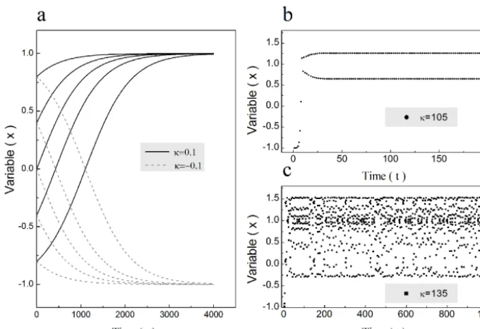
x=ν; when the rate of the system variable is zero,x˙=0. By using a numerical method, the relationship between the solution of the model, and the parameterκis shown in Fig. 2. In Fig. 2a, the system reached the same state (x=µ) dur-ing the evolution by changdur-ing the initial variable in threshold (x0∈(ν,µ)), when parameterκ(κ=0.1) was positive (black lines). The dashed lines show the condition that the system reached in the statex=ν, when the parameterκ (κ <0) was negative. In Fig. 2b, the parameter κ(κ=105) was larger than before, and the system became bifurcated. If the pa-rameterκ(κ=135) is much larger, the system will become chaotic as shown in Fig. 2c. Therefore, the parameterκ is a stability parameter, and the parametersµandνare the start and end states before and after the abrupt change (Yan et al., 2012, 2013).

Figure 3 describes an abrupt change process when the sys-tem transforms from one stable state to another. In order to simplify the model, it was divided into three sections as shown in Fig. 3, and the length of each section is marked as

n1,n2, andn3, respectively.

1. In Sect. 1, during the period before the abrupt change, the system remained in the fixed stable statex=ν. 2. In Sect. 2, the transition process, whereby the system

transformed from a stable state (x=ν) to another state (x=µ), was considered to be linear. This means that the process could be fitted by the method of the least squares. The fitting equation isx=h·i+e, wherehis the slope and reflects the rate of the amplitude over time during the transition process.

3. In Sect. 3, the system transformed to the stable state (x=µ) after the abrupt change, which is also repre-sented as the equal of the sequence.

These parameters have been computed as a piecewise func-tion:

Figure 1. The evolution of the system over time,

com-puted by rewriting Eq. (1) as its difference scheme: x_(t+1)=τ κ(xt−µ)(ν−xt)+xt, where τ=0.01 is the time step.                  ν= n1 P i=1 xi/n1

h= n1+n2

P

i=n1+1 i·xi/

n1+n2

P

i=n1+1

i2, e=h·xi−i

µ=

n1+n2+n3

P

i=n1+n2+1 xi/n3

. (2)

In Sect. 2, the linear transition process has been marked as a black line. It is fixed by two points, A and B, expressed as (xα,tα) and (xβ,tβ), respectively. Then, the slope of the linear equation is expressed as

h=xα−xβ

tα−tβ

. (3)

The location parametersαandβ have been defined to de-scribe the location of these two points as follows:

xα=α(µ−ν)+ν

xβ=β(µ−ν)+ν

. (4)

(3)

Figure 2. The evolution of the system over time, with different stability parameters: (a) the system reaches to the stable states with a different

initial variable when parameterκ= ±0.01; (b) the system becomes bifurcated when the parameterκ=105; (c) the system becomes chaotic when the parameterκ=135.

Figure 3. The abrupt change process and its sections. The three

sections are as follows: period before the abrupt change, period of abrupt change process, and period after abrupt change.

Integral Eq. (1), 1

µ−ν

x

Z

x0

₁

x−ν−

1

x−µ

dx=κ

t

Z

t0 dt

⇒ln

_x₋_ν

x−µ· x0−µ x0−ν

=κ(µ−ν) (t−t0)

⇒ x−ν

x−µ= x0−ν x0−µ

·eκ(µ−ν)(t−t0). (5)

Using the intermediate variable ξ=x0−ν x0−µ·e

κ(µ−ν)(t−t0)₌

x−ν x−µ; then,

t=t0+ 1

κ(µ−ν)ln

_x

0−µ x0−ν

·ξ

. (6)

Equation (3) is expressed by

h= α(µ−ν)−β(µ−ν)

1 κ(µ−ν)

lnx0_x0−₋µ_ν ·ξα

−lnx0_x0−₋µ_ν ·ξβ

=κ(µ−ν)2 α−β

ln ξα/ξβ =κ(µ−ν)2 α−β

lnα_β ·1−β 1−α

. (7)

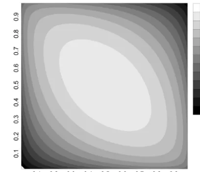
A new parameter is defined asχ= α−β ln

α β·

1−β

1−α

, which has a relationship with the location parametersαandβ. The rela-tionship is shown in Fig. 4, and parameterχ is almost con-stant when the values ofαandβare within a certain range. In this paper,α=0.2,β=0.8, andχ=0.2164.

Equation (7) is rewritten as follows:

h=κ(µ−ν)2χ . (8)

(4)

252 P. C. Yan et al.: A novel method for analyzing the process of abrupt climate change Therefore, by changing the lengths n1, n2, and n3, the

piecewise Eq. (2) could then be used to optimally fit an abrupt change process with a group of parametersϕ(h,µ,ν,

n1,n2,n3) from a sequence which occurred during a similar abrupt change.

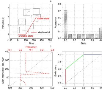
By testing a sub-sequence obtained from an entire time se-quence, a group of parametersϕ(h,µ,ν,n1,n2,n3)1could then be calculated. Also, by moving the sub-sequence onto the entire time sequence (as shown in Fig. 5a), a series of groups of parameters (ϕ1, ϕ2, ϕ3, · · ·, ϕm) could then be calculated. The process of the abrupt change could then be studied by analyzing the parameters. In Fig. 5b, in order to count the start momentν, the two states (ν=2.0 andν=4.0) are detected with higher frequency. It should be noticed that the reason the frequency of state 2 is higher than state 4 is only because the start moment (just like state 2) is counted here. In contrast, the frequency of state 4 will be higher than state 2, if only the end moment (just like state 4) is counted. To clarify, this means that two stable states exist in the time sequence, i.e., the system presents a double-peak structure. With regards to the relationship between the detecting mo-ment and the start momo-ment, as shown in Fig. 5c (blue line), the same start moment has always been detected over a long period, with the detecting moment changing from point 100 to point 500. That start moment is calculated (red line) in Fig. 5c. At point 150, the frequency is much higher than in the others. The reason being that the point is the start mo-ment of the abrupt change process of the ideal model. By uti-lizing the frequency of the start moment to judge the abrupt change, this method would improve the situations of miss-ing and false detection, which were happenmiss-ing when usmiss-ing the traditional method. Figure 5d is a phase diagram of the “start–end” states, and each point in the figure represents a detection result: thexaxis is the start state, and theyaxis is the end state.

In the vertical line (the red line), the points present a pro-cess that the start state stays constant, and the end state in-creases. This indicates that the sub-sequence has passed by the start moment during the moving process. Therefore, the vertical line represents a process in which the system devi-ates from a stable state.

In the horizontal line (the blue line), the points represent a process that the start state is increasing, and the end start state remains constant. This indicates that the sub-sequence has passed by the end moment during the moving process, which indicates that the horizontal line represents a process that the system is approaching a stable state.

The green line, which runs parallel to the diagonal, shows that the sub-sequence is in the process of an abrupt change, since both the start state and the end state are increasing, and the difference between them is constant.

It should be noted that the line running parallel to the diag-onal would vanish if the length of the sub-sequence is larger than the length of the abrupt change process. Also, the verti-cal line and the horizontal would still exist.

Figure 4. The relationship parameterχand parametersα,β, where thexaxis is parameterα, theyaxis is parameterβand the contour is parameterχ.

Therefore, based on the analysis of the result of the de-tection, the AM-ACP can be used to effectively detect the process of the abrupt change. In future studies, this method will be used to detect a real-time sequence, and the statistical characters would then be shown in order to study the abrupt change process.

3 Characteristics of abrupt change process of Pacific decadal oscillation

In this study, based on the theory of the AM-ACP, the PDO index has been analyzed to study the abrupt change process. The PDO has been considered as an important indicator of the decadal variability of the Pacific Ocean (Meehl et al., 1993), which has a strong relationship with the climate of China (Wang et al., 2013). It has been shown in many pre-vious studies, that this index has experienced several abrupt changes over the past 100 years (Mantua et al., 1997; Tsonis et al., 2007), and that all of these abrupt changes correspond to the global climate changes.

(5)

dis-Figure 5. The detection of the abrupt change process of the ideal model and the analysis of the results. (a) The ideal model (red line) and its

detection of the abrupt change process in different observed windows (black lines) with sub-sequences; (b) the statistics of the start states;

(c) the relationship between the detecting moment and the start moment (blue line), and the frequency of the star moment (red line); (d) the

phase diagram of “start–end” states.

tributed on two stable states, as illustrated in Fig. 5b. Further-more, under certain conditions, the system may have crossed over from one state to another. Such a structure has been verified several times in the climate system (Goldblatt et al., 2006; Alexander et al., 2012; Zerkle et al., 2012).

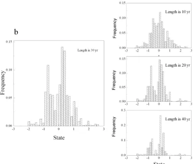
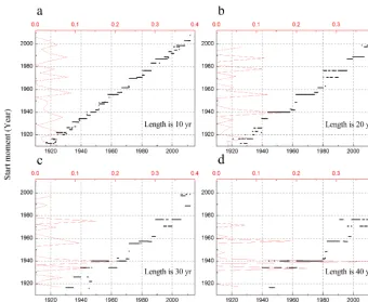
In Fig. 7, it is shown that the different start moments of the abrupt changes in the PDO index time sequence have been detected at different detecting moments. The results showed that the frequency of the abrupt change start in some years was much higher than in other years. Also, when the length of sub-sequence was set as 40 years, as shown in Fig. 7d, then the start moments of the abrupt changes that started in 1940 and 1976 were detectable for a rather long time period (de-tecting moment). These results are precisely when two tran-sitions occurred. These trantran-sitions were when the PDO index time sequence transferred from a positive phase to a negative phase in 1940, and from a negative phase to a positive phase in 1976 (Francis and Hare, 2007). The abrupt change in 1955, was detected by an abnormally smaller value of the PDO in-dex time sequence in that year. In addition, the frequency of detected abrupt changes in 1934 and 1988 was higher, which

indicated that the system did deviate, but with only a small amplitude, from a stable state.

Figure 8 shows the “start–end states” phase diagram of the PDO system during the period from 1900 to 2010, and the five clear abrupt changes are marked with five differ-ent colors in the diagram. As shown in Fig. 5d, the verti-cal and horizontal lines represent different sections of the abrupt change process. In regards to the different lengths of the sub-sequence, all five abrupt change processes have been detected. By taking a 30-year length as the set time length for example, the result was analyzed as follows.

The first abrupt change process started in 1934 (marked with blue dots), and the vertical section line which consists of blue dots in the phase diagram, is located on the left-hand side of the diagonal line. By comparing this with Fig. 5d, we concluded that this was a continuously increasing process, and had increased to a new stable state.

(6)

254 P. C. Yan et al.: A novel method for analyzing the process of abrupt climate change

Figure 6. Histogram of statistical distribution of the start state. Thexaxis refers to the statistical interval for the PDO index, and theyaxis refers to the frequency.

The third abrupt change process started in 1955 (marked with green dots), and it is located in a neighboring area of the diagonal line. By comparing this with Fig. 5d, we concluded that this was a non-abrupt change process, for example, ab-normally small values had been detected in the original time sequence.

The fourth abrupt change process started in 1976 (marked with yellow dots), and the red dots consist of a vertical line located on the left-hand side of the diagonal line. This indi-cates an increasing process to a stable state, which is similar to the abrupt change that started in 1934 marked with a blue line.

The fifth abrupt change process started in 1988 (marked with red dots), which has been divided into two sections: an approximate vertical and horizontal lines, where the vertical line indicates a decreasing process from an stable state, and the horizontal line indicates a decreasing process to an stable state.

In conclusion, the dotted line in the “start–end states” dia-gram indicates different abrupt change processes which may be included in certain stages of an abrupt change. For all of the abrupt changes detected, two changes which started in

1940 and 1976 have longer vertical lines, indicating these two abrupt changes were more severe. This is the reason why these two abrupt changes have also been detected by some other detection methods.

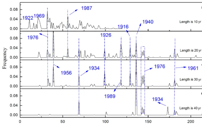
In Fig. 9, some further research is shown concerning the relationship between the persist time and the start moment of the abrupt change processes. The results indicated that the abrupt changes starting from different moments have clear differences in persist times. The abrupt changes which started in 1940 and 1976, continued for 136 and 144 months, respec-tively. This is consistent with the observations of the time se-quence of the PDO index. The abrupt change which started in 1988, continued for 120 months; the abrupt change started in 1934, continued for 70 months; and the abrupt change started in 1955, only continued for 38 months. In addition, by slid-ing the sub-sequence onto the entire time sequence, the per-sist time of each abrupt change may be detected more than once, i.e., the abrupt changes started in 1940 and 1976. The reason for this multiple detection is that such abrupt changes belong to different abrupt change processes.

(7)

Figure 7. Start moment of the abrupt change in PDO index series with different detecting moments. Thexaxis refers to the detecting moment of each sub-sequence detected, or the moment for detecting the time sequence, while theyaxis refers to the start moment. The black short line indicates the start moment of the abrupt change, which is detectable in a rather long time period; and the red line refers to the frequency of the start moment. (a–d) are the different conditions in which the lengths of sub-sequence are set as 10a, 20a, 30a, and 40a.

(8)

Figure 9. Distribution of the abrupt change persist time with the start moment. (a–d) show the different conditions in which the length of

the sub-sequence are set, which are 10a, 20a, 30a, and 40a. Thexaxis refers to the persist time of the abrupt change, theyaxis refers to the frequency of the abrupt changes that satisfies the conditions, and the characters mark the start moments of each abrupt change process.

Figure 10. Abrupt changes start at different moments than their

per-sist times. Thexaxis refers to the persist time of each abrupt change process, and theyaxis refers to the start moment.

Fig. 10, the distribution of the relationship is shown with the length of sub-sequence set as 10, 20, 30, and 40 years. The number of abrupt changes following the 1960s, significantly exceeded that before the 1960s, which reflects the fact that the climate system might have become progressively unsta-ble. In regards to the several abrupt changes occurring before the 1960s, the later the abrupt change started, the shorter the persist time of the change became. As for the abrupt changes after the 1960s, these abrupt changes can be divided into two groups, which are those lasting for more than 100 months, and those lasting for less than 50 months. In regards to the persist times, in the former group it was found to be shorter, while in the latter group the persist time was extended, and

the two groups were in a symmetrical distribution for ap-proximately 70 to 80 months. In addition, the global tem-perature continued to increase prior to 1940, and reached its peak value during the 1940s, then it remained at a lower level for the following 10 years, before beginning to slowly rise at the start of the 1950s (IPCC, 2007). This is consistent with the abrupt change in the PDO index time sequence. These facts indicated that, under the context of global warming, the oceanic system showed an evidently unstable state, and that the persist time of the abrupt changes which began after the 1950s presented a trend of becoming closer to the range of 70 to 80 months.

4 Conclusions

As the evidence of a climate system swing among different states has undoubtedly given us an opportunity to learn more about abrupt climate change events, a new method to analy-sis the process of abrupt climate change, AM-ACP, was pro-posed in this study, and the method has also provided a new perspective to research abrupt climate change.

By using an ideal mean change time sequence to simu-late the process of the abrupt change, there are three char-acteristics that can be shown: (1) multi-stable states exist in the abrupt change events, (2) the start moment of the abrupt change is detectable in different times, and (3) the “start–end states” phase diagram could be used to express the duration of the abrupt change.

(9)

transi-tion among different stable states has occurred five times over the past 100 years in 1934, 1940, 1955, 1970, and 1976, and the “start–end states” phase diagrams show the transforma-tion processes clearly. In additransforma-tion, the persist time of each abrupt change is almost constant, and the persist time be-comes shorter with global warming. After 1960s, the per-sist time gets longer when shorter than 100 months; on the contrary, the persist time gets shorter when it is longer than 100 months. With regards to the process of abrupt climate change, further work is needed to research this subject, and more evidence concerning abrupt climate change is needed in order to find a more efficacious method to research the abrupt change process. Now we may unable to accurately forecast exactly when an abrupt climate change will occur, but at least we hope that in the future we can devise a method-ology which can be used to determine whether we are in the process of an abrupt climate change, which is of great impor-tance to human society.

Acknowledgements. The authors would like to thank the anony-mous reviewers and the editors for helpful suggestions. This project was supported by National Natural Science Foundation of China (grant nos. 41175067 and 41305056), National Basic Research Program of China (grant no. 2012CB955901), and National Natural Science Foundation of China (grant no. 41375069).

Edited by: V. Perez-Munuzuri Reviewed by: two anonymous referees

References

Alexander, R., Reinhard, C., and Andrey, G.: Multistability and crit-ical thresholds of the Greenland ice sheet, Nat. Clim. Change, 2, 429–432, 2012.

Alley, R. B., Marotzke, J., Nordhaus, W. D., Overpeck, J. T., Pe-teet, D. M., Pielke, R. A., Pierrehumbert Jr., R. T., Rhines, P. B., Stocker, T. F., Talley, L. D., and Wallace, J. M.: Abrupt climate change, Science, 299, 2005–2010, 2003.

Baker, M. B. and Charlson, R, J.: Bistability of CCN concentrations and thermodynamics in the cloud-topped boundary layer, Nature, 345, 142–145, 1990.

Charney, J. G. and DeVore, J. G.: Multiple flow equilibria in the atmosphere and blocking, J. Atmos. Sci., 36, 1205–1216, 1979. Dai, X. G., Wang, P., and Zhang, K. J.: A decomposition study of

moisture transport divergence for inter-decadal change in East Asia summer rainfall during 1958–2001, Chin. Phys. B, 21, 119201, doi:10.1088/1674-1056/21/11/119201, 2012.

Feng, G. L., Gong, Z. Q., and Zhi, R.: Latest advances of climate change detecting technologies, Acta Meteorol. Sin., 66, 892– 905, 2008.

Feng, G. L., Hou, W., Zhi, R., Yang, P., Zhang, D. Q., Gong, Z. Q., and Wan, S. Q.: Research on Detecting, Diagnosing and Pre-dictability of Extreme Climate Events, Science Press, Beijing, China, 2011.

Francis, R. C. and Hare, S. R.: Decadal-scale regime shifts in the large marine ecosystems of the Northeast Pacific: a case for his-torical science, Fish. Oceanogr., 3, 279–291, 2007.

Fu, C. B. and Wang, Q.: The definition and detection of the abrupt climate change, Scient. Atmos. Sin., 16, 482–493, 1992. Goldblatt, C., Lenton, T. M., and Watson, A. J.: Bistability of

atmo-spheric oxygen and the Great Oxidation, Nature, 443, 683–686, 2006.

Goossens, C. and Berger, A.: Annual and seasonal climatic varia-tions of northern hemisphere and europe over the last century, Ann. Geo-Phys., 4, 385–400, 1986.

He, W. P., Feng, G. L., Wu, Q., He, T., Wan, S. Q., and Chou, J. F.: A new method for abrupt dynamic change detection of correlated time series, Int. J. Climatol., 32, 1604–1614, doi:10.1002/joc.2367, 2012a.

He, W. P., Wan, S. Q., Jiang, Y. D., Zhang, W., Wu, Q., and He, T.: Detecting abrupt change on the basis of skewness: Nu-merical tests and applications, Int. J. Climatol., 33, 2713–2727, doi:10.1002/joc.3624, 2012b.

IPCC: Climate Change 2007, Synthesis Report, Cambridge Univer-sity Press, Cambridge, UK, 2007.

Li, J. P., Chou, J. F., and Shi, J. E.: Complete definition and types of abrupt climate change, J. Beijing Meteorol. Coll., 1, 7–12, 1996. Lorenz, E. N.: Nondeterministic theories of Climate change,

Qua-ternary Res., 6, 495–506, 1976.

Mantua, N. J., Hare, S. R., Zhang, Y., Wallace, J. M., and Fran-cis, R. C.: A Pacific interdecadal climate oscillation with impacts on salmon production, B. Am. Meteorol. Soc., 78, 1069–1079, 1997.

May, R.: Simple mathematical models with very complicated dy-namics, Nature, 261, 459–467, 1976.

Meehl, G. A., Branstator, G. W., and Washington, W. M.: Tropi-cal Pacific Interannual Variability and CO2Climate Change, J. Climate, 6, 42–63, 1993.

Shi, N.: Meteorological statistical forecast, Meteorological Press, Beijing, China, 2009.

Stefan, R.: Ocean circulation and climate during the past 120,000 years, Nature, 419, 207–214, 2002.

Thom, R.: Stability Structural and Morphogenesis, Sichuan Educa-tion Press, Sichuan, China, 1972.

Tong, J. L., Wu, H., Hou, W., He, W. P., and Zhou, J.: Early warn-ing signals of abrupt temperature change in different regions of China over the past 50 years, Chin. Phys. B, 23, 049201, doi:10.1088/1674-1056/23/4/049201, 2014.

Tsonis, A. A., Swanson, K., and Kravtsov, S.: A new dynamical mechanism for major climate shifts, Geophys. Res. Lett., 34, L13705, doi:10.1029/2007GL030288, 2007.

Wan, S. Q. and Zhang, W.: Detection and attribution of abrupt cli-mate changes in the last one hundred years, Chin. Phys. B, 17, 2311–2316, 2008.

Wang, K., Feng, G. L., Zeng, Y. X., and Wang, X. J.: Analysis of Stable Components in Extended-Range Forecast for the Coming 10–30 Days in Winter 2010 and 2011, Chin. Phys. B, 22, 129202, doi:10.1088/1674-1056/22/12/129202, 2013.

(10)

Xiao, D., Li, J. P., and Zhao, P.:Four-dimensional structures and physical process of the decadal abrupt changes of the northern extratropical ocean-atmosphere system in the 1980s, Int. J. Cli-matol., 32, 983–994, doi:10.1002/joc.2326, 2011.

Yamamoto, R., Iwashima, T., and Sanga, N. K.: Climatic jump,a hypothesis in climate diagnosis, Meteorol. Soc. Jpn., 63, 1157– 1160, 1986.

Yan, G. H., Yan, P. C., Hou, W., and Wu, H.: A method of abrupt change process analysis based on Logistic model and its applica-tions, Acta Phys. Sin., 62, 079202, doi:10.7498/aps.62.079202, 2013.

Yan, P. C., Hou, W., and Hu, J. G.: The critical warning research of the mean time sequence mutations based on Logistic model, Acta Phys. Sin., 61, 189202, doi:10.7498/aps.61.189202, 2012. Yan, P. C., Feng, G. L., Hou, W., and Wu, H.: Statistical

charac-teristics on decadal abrupt change process of time sequence in 500 hPa, Chin. J. Atmos. Sci., 38, 861–873, 2014.