Nonlinear Processes
in Geophysics
c
European Geophysical Society 2001
Model error in weather forecasting
D. Orrell1,2, L. Smith1,3, J. Barkmeijer4, and T. N. Palmer4
1Mathematical Institute, University of Oxford, 24-29 St Giles’, Oxford OX1 3LB, UK
2Present address: Centre for Nonlinear Dynamics, Department of Civil and Environmental Engineering, University College London, Gower Street, London WC1E 6BT, UK
3Centre for the Analysis of Time Series, Department of Statistics, London School of Economics, Houghton Street, London WC2A 2AE, UK
4European Centre for Medium Range Weather Forecasts, Shinfield Park, Reading RG2 9AX, UK Received: 16 October 2000 – Revised: 15 May 2001 – Accepted: 15 July 2001
Abstract. Operational forecasting is hampered both by the
rapid divergence of nearby initial conditions and by error in the underlying model. Interest in chaos has fuelled much work on the first of these two issues; this paper focuses on the second. A new approach to quantifying state-dependent model error, the local model drift, is derived and deployed both in examples and in operational numerical weather pre-diction models. A simple law is derived to relate model error to likely shadowing performance (how long the model can stay close to the observations). Imperfect model experiments are used to contrast the performance of truncated models ative to a high resolution run, and the operational model rel-ative to the analysis. In both cases the component of forecast error due to state-dependent model error tends to grow as the square-root of forecast time, and provides a major source of error out to three days. These initial results suggest that model error plays a major role and calls for further research in quantifying both the local model drift and expected shad-owing times.
1 Introduction
Error in weather forecasting can be attributed to two causes: deficiencies in the model, and inaccurate initial conditions (Bjerknes, 1911). Since weather models are thought to be chaotic, and, therefore, sensitive to small changes in initial condition (Lorenz, 1963), much attention has focused on the latter as a limit to predictability. Techniques which have evolved to counter it include ensemble weather prediction, where an ensemble of initial conditions, within some toler-ance of the analysis (our best guess of the current state), is run forward under the model to obtain an impression of the likely range of future states (Toth and Kalnay, 1993; Molteni et al., 1996; Palmer, 2000).
While chaos certainly makes prediction difficult, it also obscures the role of model error, since as soon as a model Correspondence to: D. Orrell ([email protected])
trajectory diverges from “truth” it will presumably fall victim to the effects of chaos. Perhaps as a result, and while model error has been studied in the context of weather forecasting (Schubert and Schang, 1996; Wergen, 1992), there has not existed a satisfactory method for measuring its effect on fore-cast accuracy (Houtekamer et al., 1996). A lower bound can be obtained by comparing different models (Downton and Bell, 1988; Harrison et al., 1999; Richardson, 1997), but the models share common assumptions about the physics, and an upper bound is not known. Stochastic variation of model parameters (Houtekamer et al., 1996; Buizza et al., 1997), meanwhile, will reflect the sensitivity of the model to partic-ular parameters but not to structural deficiencies. The lack of information about model error is a problem, as it not only de-prives the model builders of feedback (Schubert and Schang, 1996; Leith, 1978) but also deprives the users, such as those involved in the pricing of weather derivatives, of a realistic understanding of forecast accuracy and makes it difficult to assess the effectiveness of procedures such as ensemble fore-casting.
Given a particular target orbit, defined as a projection into model space of a true system orbit, this paper follows Bjerknes in dividing error into two types: displacement er-ror, which is caused by the model being evaluated at a point which is displaced from the target orbit, and, therefore, is the same as initial condition error at initial time, and model error, which occurs when the model tendency differs from that of the target orbit at initial time, even though the equations are evaluated on the target orbit. (Terms are also defined in the Glossary.) Model error plays a part both in the evaluation of the model tendency, and in the analysis scheme which may, for example, lead to distortion over data-poor areas. It can be systematic and/or state dependent.
rel-−0.04 −0.02 0 0.02 0.04 −0.04
−0.02 0 0.02 0.04
t=0.00 initial ball
model is PERFECT
−−−−>
xp
yp
−0.04 −0.02 0 0.02 0.04 −0.04
−0.02 0 0.02 0.04
t=0.00 same initial ball
but model is IMPERFECT
−−−−>
xp
yp
Error wrt Model
t=0.04 ball distorts ...
−−−−>
Error wrt Target
t=0.04
still shadows
−−−−> t=0.08 ... but no drift
t=0.08 no shadow!
drift
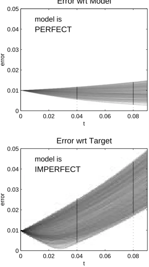
Fig. 1. Panel showing the relationship between model error, shadow
trajectories, and ensemble behaviour for a real model/system pair. The upper panels show ensemble errors with respect to the model, lower panels with respect to the target system. Model is Lorenz
1963 withr =28.1, target is Lorenz 1963 withr=28.0 (see
Ap-pendix for equations). Ensemble consists of 500 initial conditions randomly perturbed on a ball of radius 0.01. The points have been projected onto the plane perpendicular to the tangent of the target orbit. In the imperfect model scenario (lower panels), the ball has
distorted into an ellipse byt = 0.04, but the model still shadows
the target. Byt= 0.08, however, the model has ceased to shadow
within the specified radius.
evance of shadow trajectories and model error to ensemble performance can be seen in Fig. 1, which shows errors of a ball of initial conditions run forward under a model. In the upper panels, errors are expressed relative to the model, and thus correspond to a perfect model scenario. The lower pan-els show errors with respect to the true target system, and thus correspond to an imperfect model scenario. (The data are for a real model/system pair based on the Lorenz 1963 equations and described in the caption, see also Orrell, 2002). In the upper panels, the ball distorts into an ellipse but some members continue to shadow, while in the lower panels the model error causes the ellipse to drift away from the target. By timet =0.08, no trajectory remains within the initial ra-dius, and the model has ceased to shadow the target system.
If no initial condition within the tolerance can shadow, the final distribution of ensemble members will not accurately reflect reality. This effect is also seen in Fig. 2, which shows error growth of the ensemble members for perfect and imper-fect model scenarios. In the lower panel, the error growth is dominated by the model error, rather than the spread of the ensemble. The existence of a shadow trajectory, for a rel-evant tolerance, can be considered a minimal condition for ensemble schemes to be effective. In general, if model error is relatively small, then it should be possible to find shadow trajectories. If model error is large, then we will see below that the model will not in most cases shadow beyond a well-defined time. Model error and shadow times are fundamen-tally linked.
Our aim in this paper will be to develop a method to
mea-model is
PERFECT
Error wrt Model
t
error
0 0.02 0.04 0.06 0.08
0 0.01 0.02 0.03 0.04 0.05
model is
IMPERFECT
Error wrt Target
t
error
0 0.02 0.04 0.06 0.08
0 0.01 0.02 0.03 0.04 0.05
Fig. 2. Panel showing ensemble error growth with respect to the
model (upper panel) and target (lower panel). Model and target system are the same versions of Lorenz 1963 used in Fig. 1. Early stage errors relative to the model show some directions growing and others contracting. Errors with respect to the target, in contrast, in-crease at a rate related to the model error. The vertical lines indicate
the errors att =0.04 andt =0.08, which can be compared with
the corresponding panels in Fig. 1.
dimensional system due to Lorenz (1996), before moving on in Sect. 5 to full weather models, where we compare differ-ent resolution models from ECMWF. In Sect. 6 we use the techniques developed to determine the contribution of model error to total forecast error, and produce an estimate for shad-owing times of the operational forecast. Finally, in Sect. 7, we discuss how an improved measure of model error can lead to more accurate forecasts. We limit ourselves throughout to determining the magnitude of model error, and its effect on shadowing times and ensemble behaviour, but not its causes or variations in physical space, which are topics for further research.
Of course, the true state of the atmosphere is never known (indeed, this is the case with any physical system). We only know the weather through the analysis, which is sub-ject to random fluctuations, which are themselves model de-pendent. We address this issue by concerning ourselves only with shadowing the (discrete) trajectory in state space given by the analysis. If the model initial condition cannot be per-turbed so that its trajectory lies within a specified shadow radius of the analysis after a period of, say, two days, then this is indicative of model error, rather than any uncertainty in the analysis.
2 Model error and the linearised dynamics
In this section we develop a mathematical framework for studying shadow trajectories, and explore the relationship be-tween model error and the ability of the model to shadow a target orbit. A first step is to define more exactly what is meant by the target orbit. The model and the true sys-tem will normally have different state spaces (Smith, 1997). Let the model state space vector bex ∈ <n, and the system state space vector be X˜(t )in some other state space (usu-ally higher dimensional). We also assume the existence of a
C1projection operator P from the true system state space to the model state space. The target orbit is then the projection
˜
x(t )=P(X˜(t ))of the true orbit into model space. The target orbit therefore exists in model space, but it is not a trajectory of the model. Rather it is an orbit which represents our un-derstanding of truth, and is a target at which we wish to aim. The definition of a target orbit is relative to the projection operator, so changing the projection changes what we see as “truth”. In fact, the target orbit can be a projected trajectory of another model, or a series of analyses.
Now, suppose the model is given by the equation
dx
dt =G x(t )
, (1)
which specifies the model tendency in terms of the model state space vectorx ∈ <n and suppose that we wish to use this model to approximate the target orbitx˜(t )= P(X˜(t )). We further assume thatGisC1.
Model error at the pointx˜(t )can be viewed as the differ-ence between the model tendency and the tendency of the
target orbit, which is given by the tendency error
Ge x˜(t )=G x˜(t )−
dx˜(t )
dt . (2)
In general, Ge is non-zero, unless the model is perfect, so it
follows that model solutions will diverge from the target orbit at an initial linear rate. The situation, therefore, differs from that of displacement errors, which may have an initial zero or negative growth rate. Since the tendency error is evaluated on the target orbit, displacement error at that point is zero by the definition used throughout this paper.
Our definition of tendency error is essentially the same as that used in Klinker and Sardeshmukh (1992), where the tendency errors were studied in an attempt to isolate their sources in the model, or in Schubert and Schang (1996), who proposed a statistical technique for assessing error in General Circulation Models. A similiar term also appears as a resid-ual in 4D-VAR (Cohn, 1997). The tendency error provides a measure of instantaneous model error at initial time. This in-stantaneous value does not, however, determine the effect of model error on shadowing, for which we need to know how the model error interacts with displacement error as they both evolve with time over a shadow trajectory.
Consider, therefore, a model trajectoryx(t )which shad-ows the target orbit within a radiusrs for a timeτ. Since a
shadow trajectory is one which stays withinrs of the target
orbit, we have
kx(t )− ˜x(t )k ≤rs (3)
for all timest with 0 ≤ t ≤ τ. We can make a first order approximation to the forecast error by linearising around the target orbit. Let the error vector be
e(t )=x(t )− ˜x(t ), (4)
the difference between the model trajectory and the target orbit. The time dependence of the error vector is
de
dt =
dx
dt −
dx˜
dt
=G x(t )−G x˜(t )+Ge x˜(t )
=G x˜(t )+e(t )−G x˜(t )+Ge x˜(t ). (5) Now, becausex(t )was chosen to be a shadow trajectory, we knowke(t )k ≤rs. Therefore, from the Taylor series
expan-sion of G about the pointx˜(t ), we can write
de
dt ≈J x˜(t )
·e(t )+Ge x˜(t )
, (6)
where the matrix J is the Jacobean of G, and the approxima-tion isO(rs2).
Integration of Eq. (6) yields
e(τ )≈M(τ )·e(0)+d(τ ) (7)
where
d(τ )=
Z τ
0
Ge x˜(t )dt
=
Z t
0
and M(t ) is the linear propagator (Strang, 1986) of the model, evaluated along the target orbit. The approximation is againO(rs2)(Orrell, 2001), and therefore is only useful for those trajectories which shadow at a sufficiently small radius.1The vectordhas dimension distance and will be re-ferred to as the drift (or local drift, to distinguish it from any long term drift). The drift depends on the trajectory, so even if it is forced to zero in the long term (i.e. no climate drift), it may accumulate in the short to medium term. For short times, the drift is approximately equal to the error of a fore-cast initiated on the target orbit, as is easily seen by setting
e(0)equal to the zero vector in Eq. (7).
The effect of the linearised dynamics can be seen in the lower panels of Fig. 1: the ball of initial conditions is torted into an ellipse by the linear propagator M, and dis-placed by the drift d. For this particular example the lin-earised dynamics appear to hold for the entire ball of initial conditions. In general, though, the linearised dynamics apply only to those trajectories which shadow the target within ra-diusrs. Trajectories outside the shadow radius may become
severely distorted by nonlinearities. The linearised dynam-ics, restricted in this way to shadow trajectories, can there-fore hold even when arbitrary non-shadowing perturbations become highly nonlinear.
To sum up the results of this section, we have used the lin-earised dynamics to separate out the effects on shadow tra-jectories of model error, in the drift vector, and the effects of displacement error, in the linear propagator acting on the initial displacement. The model itself need not be linear for the linearised dynamics to hold to good accuracy. We next use the linearised dynamics to develop a simple shadowing law which underpins the link between shadowing and model error.
3 The shadow-drift law
In this section, we use the dynamics, linearised about the tar-get, to develop a simple relationship between model error, as measured by the drift, and expected shadow performance of the model. Details of the derivation, along with examples, are given in Orrell (2001). Here we sketch the argument. Sup-pose that the linearised dynamics provide a good approxima-tion for points which shadow within a shadow radiusrs. Such
points, acted on by the linearised dynamics, will be distorted into a portion of an ellipse by the linear propagator, and dis-placed by the drift. The model should, therefore, cease to shadow when the resulting distribution exceeds a distancers
from the target. For a given driftd(τ )the radiusrs can be
calculated explicitly using a Lagrangian method, and to first order satisfies the relation
n X
i=1
d(τ )·ui(τ )2
1+σi(τ ) 2
=rs2, (9)
1Small here is defined by the Taylor expansion ofG, not by the
observational uncertainty.
where σi(τ ) is the singular value corresponding to the
sin-gular vectorui(τ ). This relationship has been successfully
used to estimate shadow times as a function of radius for a range of simple models, and can hold even in cases when the models are highly nonlinear over the shadow period.
For weather models, it is of course impossible to calculate all the singular vectors. Nevertheless, if the drift is uncor-related with the singular vectors, then we can establish an approximate upper bound on shadow times. We assume that the model is either dissipative or preserves volume in state space over timeτ, so
n Y i=1
σi ≤1. (10)
Consider first the volume preserving case, where equality holds in the above equation. By solving the constrained min-imisation problem, again using a Lagrangian technique, the expected value of the sum in Eq. (9) is seen to have a mini-mum in the case whereσi =1 for alli. Therefore
* n X i=1
d(τ )·ui(τ )
2
1+σi(τ )
2
+
≥ d(τ )
2
4 . (11)
For a dissipative model, the inequality is replaced by strict inequality.
Combining Eqs. (11) and (9), we derive the shadow-drift law, which provides a link between model error, as measured by the drift, and shadowing. Suppose the drift is uncorrelated with the singular vectors. Then an approximate lower bound2 on the radiusrs within which the model may be expected to
shadow for timeτ is given byrm(τ ), where
rm(τ )=
1
2d(τ ). (12)
If the model is only weakly dissipative over the shadow time, then the shadow radius will approach the bound, so
rs(τ )≈
1
2d(τ ). (13)
This relationship tends to hold when shadow times are rela-tively short, either as a result of high model error or a small shadow radius.
The shadow-drift law shows that the drift is a useful mea-sure, not only of model error, but of a model’s ability to shadow. The drift, therefore, serves as a computationally in-expensive measure of model quality (it is far easier to calcu-late the drift, which is just a sum of forecast errors, than it is to search for actual shadow orbits). The shadow-drift law will of course fail under certain circumstances and is most applicable when model error is relatively large. Our aim in this paper is not so much to verify the shadow-drift law for weather models, as to use it as one of several tools to inves-tigate model error.
2By “approximate lower bound”, we mean that the expected
ra-dius may be larger thanrm(τ ), but if it is smaller, then the difference
0 0.05 0.1 0.15 0.2 0.25 0.3 0.35 0.4 0.45 0.5 0
0.1 0.2 0.3 0.4 0.5 0.6 0.7 0.8
t
error
Shadowing for Lorenz Model
forecast shadow drift
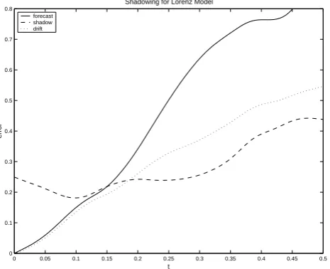
Fig. 3. Errors for forecast (solid line), shadow trajectory (dashed
line), and drift (dotted line). Model is 8D Lorenz constant model
withF = 9.62, system is 40D two-level Lorenz withF = 10.0.
Shadow tolerance is 0.3. Drift and shadow are defined in Sect. 2.
To recap, the evolution of a shadow trajectory can be ap-proximated by linearising the model equations around the target orbit. Provided the shadow radius is sufficiently small, the linearised dynamics can hold for long periods of time, even if the model is highly nonlinear. The drift serves as a measure of model error, and, therefore, of model quality. From the shadow-drift law, the drift divided by two provides an approximate lower bound on shadow radius. Just as no one can escape their shadow, no shadow trajectory can, on average, escape the effect of drift. In the next section, we illustrate these ideas on a particular model/system pair.
4 Illustration with the Lorenz 1996 system and models
Before moving on to real weather models, we first demon-strate the above points using a medium-dimensional model and true system. The model, which we will refer to as the constant model, will be the Lorenz one-level (Lorenz, 1996) model withn=8 (the equations are given in the Appendix). This 8-dimensional model consists of 8 variablesxi, which
can be interpreted as an atmospheric quantity like tempera-ture distributed around a circle. The equations simulate ad-vection, internal damping, and a constant external forcing. The system which we will treat as truth (Lorenz two-level withn = 8, m = 4 and F = 10) also has 8 large-scale variablesx˜i, but the forcing is different for each variable and
varies with time, depending on an additional thirty-two inter-coupled fine-scale variablesy˜iwhose motion is governed by
a similar set of equations. The situation is, therefore, anal-ogous to that encountered in real weather models, where a parameterisation (the constant forcing) is adopted to model convective-scale fluctuations (the fine-scale variables). The projection operator in this case retains only the 8 large-scale variables, so P(x˜,y˜)=x˜.
In order to discuss error magnitudes, we must first intro-duce a metric3. For this example the metric will be the L2 norm in the large-scale variables. Other norms are possi-ble, with the proviso that the model variables are fully rep-resented. For example, if the norm was the magnitude of only the first large-scale variablex˜1, then any vector with first componentx˜1=0 would be indistinguishable from the zero vector. This would violate the usual definition of a metric, and lead to difficulties in interpretation since a model could shadow under such a norm by trackingx˜1while completely distorting every other variable.
The solid line in Fig. 3 shows the growth in L2 forecast er-ror for a particular run. Note the non-zero slope of the erer-ror growth at initial time. While initial condition error can be re-duced to zero by choosing the perfect starting point (Judd and Smith, 2001), this is not the case for model error. The drift remains close to the forecast error until aroundt = 0.15. The figure also shows a shadow trajectory for a shadow ra-dius of 0.3. It was determined using an optimisation pro-gram that searches over initial displacements for the one with the longest shadow time; in this case about 0.34 time units, which is typical for this model. The ratio of drift to shadow radius, averaged over many separate runs, is 1.74, which is less than 2 in accordance with the shadow-drift law.
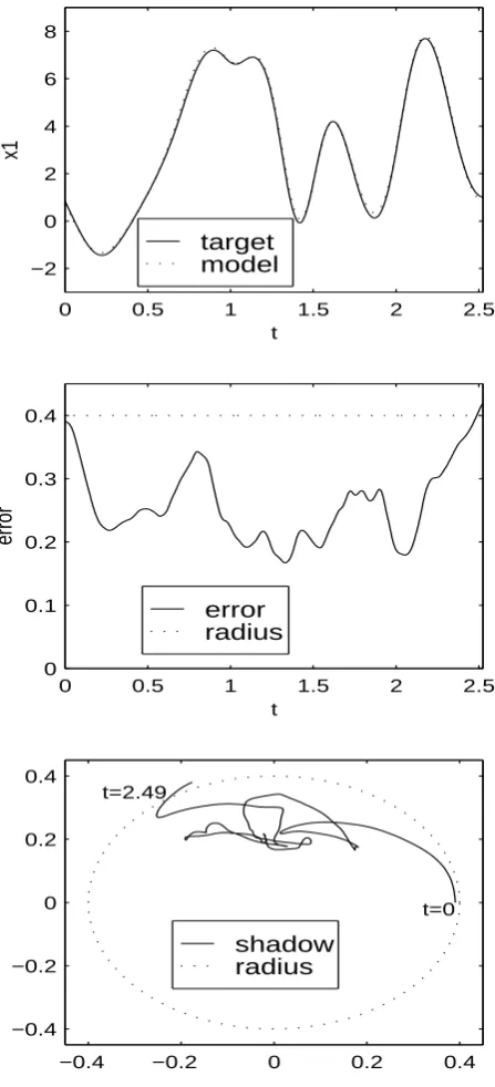
It was stated above that the shadow-drift law does not rely on the model or system being linear. Figure 4 shows a long shadow trajectory for another variant of the Lorenz model which replaces the constant model’s constant parameterisa-tion of the forcing with a term that varies linearly withx
(we refer to it here simply as the improved model, see Ap-pendix). The upper panel shows the first component of the model compared with the first component of the target; the two are nearly indistinguishable over the shadow period. The middle panel shows the L2 error as a function of time. The lower panel is an attempt to picture what is going on in 8-dimensional space. The displacement vectors have first been projected onto the hyper-plane normal to the target orbit. The radius of each point is then calculated as the displacement of the shadow trajectory from the target orbit, while the angle is the angle of the displacement at that time with the original displacement. The shadow trajectory starts near the extreme radius 0.4 on the right-hand side, then exits on the left-hand side after 2.49 time units. The trajectory clearly does not follow a linear path, yet the ratio of drift to shadow radius is 1.40, and the average for the model is 1.28, in agreement with the shadow-drift law. The linearised dynamics need not predict the exact path of such a trajectory in order to predict, to a good deal of accuracy, the conditions under which such a shadow trajectory can be expected to exist.
3One might ask why a metric is necessary if errors can be
0 0.5 1 1.5 2 2.5 −2
0 2 4 6 8
t
x1
target model
0 0.5 1 1.5 2 2.5
0 0.1 0.2 0.3 0.4
t
error
error radius
−0.4 −0.2 0 0.2 0.4
−0.4 −0.2 0 0.2 0.4
t=0 t=2.49
shadow radius
Fig. 4. Shadowing trajectory for improved model. Upper panel
shows first component of target and model over shadow period. Middle panel shows error over all components. Lower panel is in polar coordinates with radius the displacement from target orbit, and angle with respect to initial offset. The circle of radius 0.4 rep-resents the shadowing radius. The shadow trajectory starts near the extreme radius 0.4 on the right-hand side, then exits on the upper left-hand side at time 2.49 units, after following a highly nonlinear path. The linearised dynamics cannot predict the exact path of the shadow trajectory, but can predict the conditions under which such a trajectory can be expected to exist.
Figure 5 shows the average ratio of drift to shadow ra-dius for a number of shadow experiments using the constant and improved models, for different forcingsF and shadow
2 3 4 5 6 7 8 9 10 11 12
0 0.5 1 1.5 2 2.5
F
drift/radius
con r=.2*F/10 con r=.4*F/10 lin r=.2*F/10 lin r=.4*F/10
Fig. 5. Ratio of drift to shadow diameter for shadow trajectories
for the constant and improved Lorenz models as a function of
forc-ingF. Shadow radius is scaled with forcing as shown in legend,
so as to stay in proportion with the attractor diameter. Results are determined by averaging over 20 cases. All models conform to the shadow-drift law with a maximum error of 5 percent (though the shadow-drift law actually refers to expected shadow radius, while here we have treated it as fixed). The ratio is near or slightly above 2 at lower values of forcing where the models are only weakly dis-sipative, in accordance with Eq. (13).
radii.4 The shadow-drift law holds in all cases, in that the ratio is less than or near 2, with a maximum error of about 5 percent (though here we have fixedrs, which is slightly
different from the derivation above). The ratio is near 2 at lower values of forcing where the models are only weakly dissipative, in accordance with Eq. (13).
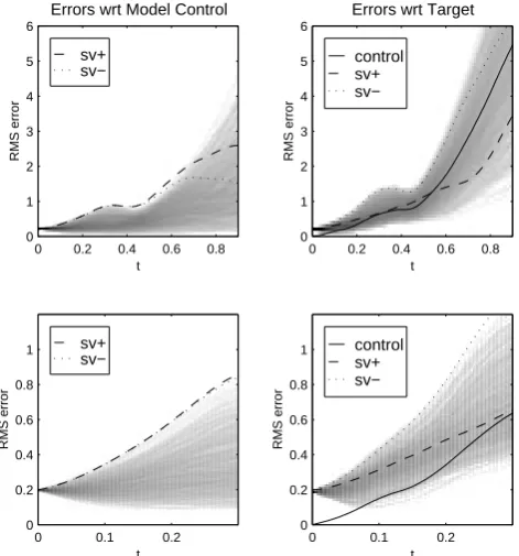
One important consequence of model error is its effect on ensemble performance. It was already seen in Fig. 1 that model error can result in the entire ensemble drifting away from the target. That figure was for a low-dimensional model; in higher dimensions it is more difficult to visualise the effect of model error, but certain deductions can be made by examining the magnitude of forecast errors. Figure 6 shows ensemble errors for the constant model, and can be compared with Fig. 2. In the upper left panel, perturbations of size 0.2 are added to the constant model’s initial condition in the positive and negative directions of the leading singular vector (optimised for time 0.34). Relative to the control fore-cast, these perturbations have grown at time 0.34 by about a factor 5.0. In addition, shown in the background is the den-sity of errors found by randomly perturbing the initial con-dition by an amount of 0.2 and taking a histogram of the resulting errors over 1000 runs. The singular vector pertur-bations give maximum displacement fort = 0.34, as they should by construction (for infinitesimal perturbations), but
4Details of the experiments are given in Orrell (2001). The
t
RMS error
Errors wrt Model Control
0 0.2 0.4 0.6 0.8
0 1 2 3 4 5 6
sv+ sv−
t
RMS error
Errors wrt Target
0 0.2 0.4 0.6 0.8
0 1 2 3 4 5 6
control sv+ sv−
t
RMS error
0 0.1 0.2
0 0.2 0.4 0.6 0.8
1 sv+
sv−
t
RMS error
0 0.1 0.2
0 0.2 0.4 0.6 0.8
1 control
sv+ sv−
Fig. 6. Forecast errors for Lorenz model/system. The left panels
show the effect of perturbing the constant model’s initial condition by 0.2 along the first singular vector (dashed) and its negative (dot-ted). Optimisation time for the singular vectors is 0.34. The back-ground contour shows the effect of random perturbations. Errors are relative to the unperturbed forecast. The right panels shows the effect of the same perturbations, but errors are now relative to the target orbit, and include the effect of model error. Lower panels are zoomed views near initial time.
not for other times. The lower left panel is a zoomed view near initial time.
The panels on the left correspond to a perfect model sce-nario. In the panels on the right, where errors are shown rel-ative to the target orbit, the situation is different. As in Fig. 2 for the 3D model, the error relative to the control is not rep-resentative of the error relative to truth. The growth rate of the singular vector perturbations is similar to that of the un-perturbed forecast, and neither the positive nor the negative perturbation effectively offsets model error compared to the random displacements. As noted in Toth et al. (1996), with regards to ensembles which perturb only initial conditions, the ensemble strategy will work only if the models are good enough that model-related errors do not dominate the final error fields. Perfect model experiments will always be ex-tremely misleading in this regard.
These demonstrations on the Lorenz model/system pairs show that model error, as measured by the drift, affects both shadow times and ensemble performance, and can be a ma-jor contributor to forecast error. The question then remains whether operational forecast models are in a low model er-ror or high model erer-ror regime. Referring to Eq. (7), a fair amount is known about the linear propagator M for such models, due to the investigations into singular vectors and
the directions of the fastest growth for perturbations in initial conditions (Buizza and Palmer, 1995). The neglected part of the equation is the driftd: we are in the odd situation of knowing more about the first order term than the zeroth order term!
5 Error in weather models
To begin the analysis of model error for operational weather models, we first compare the T42 and T63 models, taking the higher resolution TL159 to define the target (the num-ber refers to the spectral truncation, while the L in TL159 denotes the linear grid on which physics is computed). Fol-lowing Rabier et al. (1996), the vector used to describe the atmospheric statexat a particular time is
x=(u, v, T ), (14)
where u andv are the zonal and meridional wind compo-nents, andT is the temperature. The choice of norm will be the energy norm, defined as
hx,xi = 1 2
1
Z
0
Z Z
6
u2+v2+CpT 2
Tr !
d6∂pr
∂η dη. (15)
The energy norm equals the sum of the kinetic energy of the wind and the potential energy stored in the temperature, and is the same as the total energy used in Rabier et al. (1996) but with the relatively small surface pressure component omit-ted.Tris a reference temperature,pr is a reference pressure,
andCpis the specific heat at constant pressure for dry air.6
is the horizontal domain, taken here to be northwards of 30 degrees, andηis the vertical coordinate.
The energy norm was chosen because it provides a fairly global measure of the model variables (Buizza and Palmer, 1995). Norms are often picked to represent more specific quantities such as the temperature over a particular region. Our aim here, however, is to use the norm as a diagnostic tool, which measures the relative contributions of model er-ror and displacement erer-ror, and the energy norm is suitable because it gives a reasonably complete picture of the atmo-spheric state. This is in contrast to more specific norms, such as the 500 mPa height metric, which considers the model state only at a specified level, and would fail to illustrate how model error at lower or higher levels feed into that level.
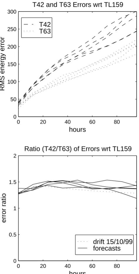
The upper panel of Fig. 7 shows forecast energy norm er-rors of five different five-day forecasts starting at different dates. For comparison, the typical size of ECMWF ensemble perturbations, when based only on initial singular vectors, is about 45 units on this scale. The model trajectories diverge from the target orbit (TL159) at a fairly constant rate, with T63 consistently performing better than T42 as one might expect. The lower panel shows the ratio of T42 errors to T63 errors, which remains quite uniform.
0 20 40 60 80 0
50 100 150 200 250 300
hours
RMS energy error
T42 and T63 Errors wrt TL159
T42
T63
0 20 40 60 80
0 0.5 1 1.5 2
hours
error ratio
Ratio (T42/T63) of Errors wrt TL159
drift 15/10/99
forecasts
Fig. 7. The upper panel shows T42 (dashed) and T63 (dotted)
fore-cast errors at starting dates 15 October 1999, 15 November 1999, 22 December 1999, 15 January 2000, 15 February 2000 (all at 12 GMT). Errors are computed in the energy norm, relative to TL159. The lower panel shows the ratio of the magnitudes of T42 and T63 errors, where each is again taken relative to TL159. Also shown is the ratio of the drifts.
fields, and the “balance” requirements forced on the initial state of the model. For the forecasts considered here, the mis-match is about 40 energy units for T42 and 30 for T63. This allows the possibility that the mismatch is responsible for the divergence of forecasts: the small initial error is magnified by the nonlinear dynamics, and the problem is not model er-ror but sensitivity to initial conditions. If that were the case it would be possible to shadow for extremely long times, since
the negligible model error could be counteracted by an ap-propriate choice of initial condition near the projected state.
From the forecast alone, we cannot separate out the ef-fects of model error and initial condition error, since the two will convolute. Therefore, we estimate the drift, following Eq. (8). A number of short, 12-hour forecasts were made with T42 and T63, starting at 12-hour intervals along the TL159 forecast. The results were then integrated numeri-cally (essentially a vector sum) to give the drift. Figure 8 shows how the drift accumulates with time for T42 and T63. The ratio of the drifts is also shown in the lower panel of Fig. 7; as for the forecasts, it is nearly constant at 1.4 over the forecast time.
If model error were truly negligible, then we would ex-pect the drift to be smaller than the forecast error, since the tendency difference is always calculated on the target orbit where displacement error is minimal. In fact, the magnitude of the drift is close to the magnitude of the forecast error. At times it is even larger: the reason appears to be that there is an initial spin-up error associated with each short forecast, which may be an artefact due to the initial mismatch. Tests with different time steps show that the drift calculation is de-pendent on step size, and that the magnitude of the error is about 20 units per short forecast.
This spup error, whose signature is a lack of scale in-variance in the drift calculation, appears to be an unavoid-able feature of the inter-model comparisons. It means that a portion of the drift is due to spin-up effects, and the calcu-lated drift is artificially high. We will therefore attempt to deal with it using two methods, and note that the same prob-lem does not occur in the next section, where the operational forecast is compared with the analysis, and the drift calcula-tion is seen to scale with time step.
The first approach is to reduce the drift by the errors in-curred during each small forecast. For example, the drift calculation over 48 hours involves four short forecasts, so compared to a normal forecast there are three additional mis-match errors of 20 units each. We could, therefore, correct the 48 hour drifts by 60 units, giving a drift of 156 units for T42 and 99 units for T63.
The second approach is shown in Orrell (2001) and is ap-plied in cases where model error is high. Whenever a strong spin-up error is present, the drift calculation will be depen-dent on step size, because the model error is largest near ini-tial time. To circumvent the problem we can linearise the error around the model control rather than the target orbit. If this is done, the control error at 48 hours serves as a proxy for drift at that time, giving a result of 168 units for T42, and 114 units for T63. The two approaches give similar results.
0 20 40 60 80 0
50 100 150 200 250 300 350 400
hours
RMS energy error
T42 Shadowing wrt TL159
forecast shadow drift radius band
0 20 40 60 80
0 50 100 150 200 250 300 350 400
hours
RMS energy error
T63 Shadowing wrt TL159
forecast shadow drift radius band
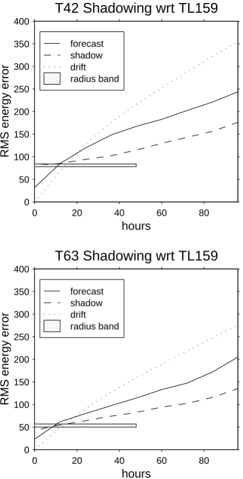
Fig. 8. The upper panel shows a plot of T42 errors with respect
to TL159 for starting date 15 October 1999. Solid line is the fore-cast, dashed line is the shadow trajectory which minimised error at 48 hours, dotted line is the drift. The uncorrected drift is in places larger than the forecast error, due to a spin-up error which is prob-ably caused by truncation error. The two estimates for the lower bound on shadow radius, computed using estimates of the drift, are shown by the shaded region. Errors are computed in the energy norm, relative to TL159. The lower panel shows the same for T63.
nonlinear within a day or so (Gilmour, 1998; Gilmour et al., 2001). For shadow trajectories, however, the linearisation is expected to hold for longer times. It therefore seems reason-able to expect that the shadow-drift law will apply.
The shadow-drift law states that the expected shadow ra-dius for a set time should be greater than or equal to half the
drift over that time. As mentioned above, there are two meth-ods for estimating the drift given the initial mismatch errors. If we correct the drift by subtracting the initial errors, we ob-tain an expected minimum shadow radius of about 78 units for T42, and 50 units for T63. If we use instead the control error as a proxy for drift, we find a radius of 84 units for T42, and 57 units for T63. The results of the two different methods are shown by the shaded region in Fig. 8.
As noted above, the drift results in the inter-model com-parison are somewhat compromised due to the initial errors; it could in principle be the case that the drift vector is due to the truncation error being consistently in the same rapidly growing direction, so that the error builds with time. Were this the case, and if model error was in fact small, then it should be possible to find trajectories which shadow for two days with a much smaller shadow radius than given above. The only way to test this is to search for actual shadow tra-jectories.
An algorithm, originally designed to find so-called sen-sitivity perturbations to offset forecast errors (Rabier et al., 1996), was employed to find such trajectories. Figure 8 shows the resulting trajectories for T42 and T63. The code uses a Newton-method optimisation scheme to reduce the cost function given by the forecast error at two days (Ra-bier et al., 1996). The step direction for each iteration is de-termined by calculating the adjoint (Dimet and Talagrand, 1988), which gives the gradient of the cost function. A total of fifty iterations were performed in each case. At time two days, the minimised error of the T42 forecast is 114 units, while for T63 it is 82 units. These are consistent with the approximate bound obtained using the shadow-drift law, in that the optimisation routine fails to find a trajectory which shadows for two days at a smaller radius than the bound. It appears that the model, not sensitivity to initial conditions, is the dominant source of error.
Trajectories with longer shadowing times may exist, as the method used is not perfect. Nevertheless, the fact that the shadow times are in accordance with the shadow-drift law increases confidence that it is the drift which limits maxi-mum shadowing times on these length scales. Since a typical shadow tolerance for assimilation purposes would be of the same order as the analysis variance, i.e. 45 units, it appears that the T42 and T63 models fail to shadow TL159 at that radius after about a day.
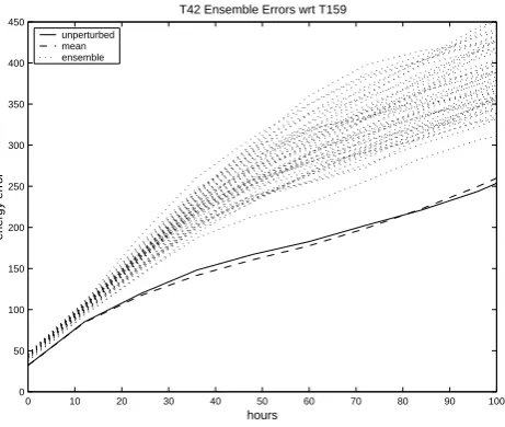
Figure 9 shows errors for an ensemble of 50 displaced T42 initial conditions, again with respect to TL159. The ensem-ble was generated by adding scaled displacements in the sub-space of the leading 25 singular vectors. The results can be compared with the lower panel of Fig. 6 for the Lorenz system; once again, no ensemble member manages to off-set model error, and the error in the ensemble mean closely tracks the error in the unperturbed forecast. (This ensemble did not contain any stochastic variation of model parameters or other simulation of model error, Buizza et al., 1997).
0 10 20 30 40 50 60 70 80 90 100 0
50 100 150 200 250 300 350 400 450
hours
energy error
T42 Ensemble Errors wrt T159
unperturbed mean ensemble
Fig. 9. Plot of errors wrt TL159 for a T42 forecast (solid line),
an ensemble of initial conditions (dotted) and the ensemble mean (dashed).
significant; a conclusion also borne out by the behaviour of the ensemble. Since one might expect models to be more like one another than like the analysis, this raises the suspicion that model error will be large relative to the analysis. In the next section we investigate whether this is the case.
6 The ECMWF operational model
We now use the techniques developed so far to estimate how long the ECMWF operational model can shadow the anal-ysis. The analysis is, therefore, used as the target orbitx˜(t )
(in, of course, a discrete form). Figure 10 shows error growth for a single forecast, along with the drift. The drift was cal-culated by summing short 6-hour forecasts for the first day to capture the fast initial growth, followed by 24-hour fore-casts for days 2 and 3. Unlike the inter-model comparisons, there is no initial mismatch error, since both the model and the analysis are at the same resolution. In addition, the cal-culation is not sensitive to step size, so summing 6, 12 or 24-hour forecasts gives similar results. This can be seen, for example, by the fact that the drift over one day, calculated by summing four 6-hour forecasts, agrees closely with the fore-cast error at 24 hours, which would be the value of the drift if a 24-hour step were used. Spin-up errors, whose signature is a strong time-step dependence in the drift calculation, are not present to a noticeable extent.
The drift closely tracks the forecast error out to three days, in a manner compatible with high model error, and the ini-tial slope is about three times greater than that for T63 versus TL159. An interesting feature of this graph is the similarity of the forecast error growth and the drift; both have a pro-nounced negative curvature. Error growth in chaotic systems is typically expected to be exponential-on-average (see, how-ever, Smith, 1994; Smith et al., 1999).
0 10 20 30 40 50 60 70
0 100 200 300 400 500 600
energy error
forecast drift
Fig. 10. Plot of TL319 forecast error (solid line) with respect to
analysis. Also shown is the drift (dotted). The drift is calculated using a time step of 6 hours for the first day and 24 hours for days 2 and 3.
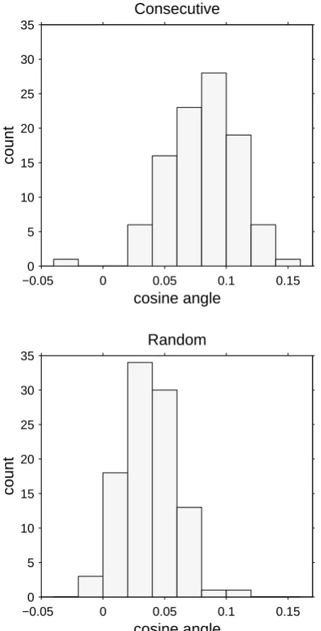
The shape of the curve makes more sense when we ex-amine the nature of the short forecast errors which make up the drift calculation. Figure 11 shows histograms of the co-sine of the enclosed angle of the 24-hour error vectors, for consecutive and randomly chosen days over a hundred day period. The mean for the consecutive days is 0.081, so they are nearly orthogonal (not surprising since the variance of the dot product of random vectors inndimensions is approx-imately 1/n). Note, though, that the distribution for consec-utive days in the upper panel is shifted significantly to the right of the distribution for random pairs of days, implying that drift is persistent on a time scale of one day; we return to discuss the fact that neither are mean zero below.
We can use the information in this distribution to build a theoretical equation for model error.5 Suppose that the 24-hour drift has average magnitudedm, and that the cosine
an-gle for consecutive days has meancm (we assume that
cor-relations become negligible for periods of over one day). By summing consecutive 24-hour drift vectors, the theoretical value of the total drift is found to be
d(t )=dm r
t
24 1+2cm
−2cm, (16)
wheretis the time in hours.
Figure 12 shows RMS forecast error over five starting dates, along with the model error as estimated using Eq. (16) withdm = 315 and cm = 0.081, which were the average
values over the sample. The theoretical model error curve,
5Even for a perfect model, non-exponential growth in the
−0.05 0 0.05 0.1 0.15 0
5 10 15 20 25 30 35
cosine angle
count
Consecutive
−0.05 0 0.05 0.1 0.15
0 5 10 15 20 25 30 35
cosine angle
count
Random
Fig. 11. Upper panel shows the normalised dot product (cosine of
angle) for 24 drift vectors at consecutive days over a 100 day period from 15 Oct 1999. Lower panel shows the same for 100 randomly chosen pairs of days from the same period.
shown as the solid line, closely matches the forecast errors up to a time of about three days. The magnitude of forecast error up to three days can, therefore, be estimated from just two numbers: the average 24-hour drift, and the average co-sine angle between consecutive drift vectors (both of which are fairly constant quantities, at least within this sample).
The fact that the forecast error curve agrees so well with the drift curve provides a strong argument that the drift cal-culations are accurate and correctly describe the model error relative to the analysis. Of course, one could still argue that this correspondence is only coincidental, and that forecast er-ror is really caused by displacement erer-ror. To do so, though,
would mean that growth rates would have to vary with time in a highly complicated manner, since displacement error oth-erwise results in exponential-on-average growth, as opposed to the square root growth which is actually seen. The as-sumption that model error is high, and that errors over the first few hours are a natural and expected effect of the model rather than anomalies due to some property of the analysis or the forecast, provides a simpler and more direct paradigm for this form of error growth.
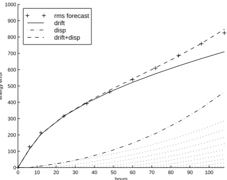
Displacement error will, of course, still play a role. The convolution of model error and displacement error will be complex, but a rough picture can be obtained by assuming that on top of the model error, an additional displacement er-ror term, which is initiated by the model erer-ror, is added to the drift. Consider, for example, the following argument. The drift calculation is performed by summing a series of short forecast errors. We then suppose that each of these errors creates a displacement which magnifies exponentially with a doubling time of 2.5 days (see Lorenz, 1969, and references thereof). Therefore, the model error over the first six hours leads to a displacement, which then grows at an exponential rate from that time on. The next six hours brings another dis-placement which will also magnify at the same rate. These displacement error curves, initiated every 6 hours, are shown at the bottom of Fig. 12. Each curve starts with magnitude zero, because it represents an error in addition to that error due to the original displacement. Summing each of these curves, and assuming orthogonality due to the dimension of the space, gives the total displacement error curve shown as the dot-dash line. When this displacement error is added to the model error, again assuming orthogonality, we arrive at the upper dashed line, which is an excellent fit to the true forecast error.
The plot is not meant to be an accurate representation of how model error and displacement error convolute. We aim merely to show that the difference between the calculated drift and the observed forecast errors is consistent with a sec-ondary displacement error. It also seems reasonable, though, that forecast error, being a mix of model error and displace-ment error, could be loosely viewed as the sum of square root and exponential growth curves. The resulting curve has an initial negative curvature phase, followed by a nearly linear growth phase in the medium range, before eventually satu-rating. Interpolating Fig. 12 forward, the model error and displacement error portions become roughly comparable in magnitude after about five days, though saturation effects may also come into play by that time.
The displacement error curve, being a sum of lagged ex-ponential terms, is not quite an exex-ponential itself. If the e-tupling time is 1/a(so the doubling time islog(2)/a), then the displacement error generated by the drift is seen to be
κ
r
1 2a(e
at−1)(eat−3)+t , (17)
where
κ = lim
1t→0
d(1t )
√
0 10 20 30 40 50 60 70 80 90 100 0
100 200 300 400 500 600 700 800 900 1000
hours
energy error
rms forecast drift disp drift+disp
Fig. 12. Plot showing how forecast error is consistent with a
combi-nation of model error and resulting displacement error. The + signs shows TL319 RMS forecast errors, with respect to analysis, over five different starting dates. Solid line is the theoretical approxi-mation for model error from Eq. (16). Dotted lines at bottom show series of displacement error curves initiated by the model error after each 6-hour period. Dot-dash line is the sum of the displacement er-ror curves, assuming orthogonality. The dashed line which closely matches the data is the sum of the model error and displacement error curves, again assuming orthogonality. The dates used for the forecast error were 15 October 1999, 15 November 1999, 22 De-cember 1999, 15 January 2000, 15 February 2000, all at 12 GMT.
which can be estimated, for example, from the 6-hour drift (the limit will exist if the drift varies with the square root of time). Note that the exponential growth is assumed to be orthogonal to the initial displacement, which differs slightly from the usual definition of doubling times.
Curves similar to those of Fig. 12 can be constructed to model 500 mPa height errors up to 5 days. In this case the square root curve usually only dominates for a day or so, rather than for three days as for total energy. As mentioned above, however, the 500 mPa height is an incomplete mea-sure of the atmospheric state, and fails to reflect total error growth (Orrell, 2002a). A similar effect is seen when, for example, error is measured over only a single variablexi in
the Lorenz model, instead of allxi. If the aim is to assess the
relative magnitudes of model error and displacement error, then the metric needs to be reasonably global.
Given the drift calculation, we can estimate shadow times using the shadow-drift law. The mean 24-hour drift over the days that were tested was 315, while the mean 6-hour drift was 138. An upper estimate of shadow time from the 6-hour drift for a radius of 45 units is then about four hours. This result is definitely on the low end of what has been consid-ered the likely range, and has implications for forecast tech-niques, such as variational assimilation (Courtier and Tala-grand, 1994), and ensemble forecasting.
The fact that model error affects ensemble schemes is not in doubt (Toth et al., 1996; Houtekamer et al., 1996), and is
clearly demonstrated for low, medium and high dimensional models in Figs. 2, 6 and 9. The shadow estimate implies that no member of an ensemble of initial conditions, perturbed by a radius of 45 units, would be expected to remain within the same radius of the analysis for more than a few hours, and neither would any trajectory initiated within the convex hull of the ensemble. If true (and we suggest below ways to verify it), this is very far from the nearly-perfect model scenario on which many ensemble schemes are based (Toth et al., 1996; Buizza et al., 1999), where model error is as-sumed to be small, relative to initial condition error, over the near to medium range. It is also consistent with the cal-culated ensemble spread tending to be too small (Toth and Kalnay, 1993), and the observed flaws in rank histogram statistics (Palmer, 2000). The same concern may also apply to ensemble schemes which include perturbations to model parameters (Houtekamer et al., 1996; Buizza et al., 1997), since such perturbations cannot address structural imperfec-tions in the model.
The correlation between successive 24-hour drift vectors, while not large, can still be used to improve the forecast. Suppose we are making a 24-hour forecast, and we know the drift dp from the preceding 24 hours. If the 24-hour forecast givesd, and we assume that the cosine angle with
dp is cm, then vector algebra shows that using d −cmdp as the corrected forecast yields a fractional improvement of 1−p1−c2
m. Forcm = 0.081 the method was shown to
yield an average correction over the days that were tested of 0.33 percent, however, it may be possible to increase this by looking, for example, at 6-hour drift vectors, and searching for higher order correlations.
An unexpected result was that the cosine angle of ran-domly chosen 24 hour drifts in Fig. 11 had a mean of 0.038. There seems to be a component of the drift which is at the least seasonal (and could be removed by post-processing). It would be interesting to quantify the long-term climate drift, which is expected to be effectively zero.
Of course it should not be implied that, even if model error is a major source of forecast error, further observations are of no consequence, nor that improving them will not affect forecast accuracy. All we can conclude is that making small displacements around the initial condition will not offset the model error and produce a shadow trajectory beyond a cer-tain time. Model error will impact the interpolation scheme incorporated in the analysis procedure (Daley, 1991); if the resulting analysis is unusually deficient over data-poor ar-eas, then this form of model error will affect performance elsewhere. The error will not be correctable through small displacements, but could be treated by improving the obser-vations (or improving the model interpolation scheme).
7 Conclusions and future work
placed on the initial condition as a source of error in weather forecasting. While the effects of chaos eventually lead to loss of predictability, this may happen only over long time scales. Exponential-on-average error growth does not neces-sarily imply rapid error growth. In the short term it is model error which dominates, and which must be considered in any scheme of quality control.
In this paper, we have promoted the use of local model drift as a measure of model quality. The model drift is easily calculated, is a good measure of model error, and, through the shadow-drift law, provides a lower bound on expected shadow radius. Unlike RMS forecast error, it distinguishes between model error and displacement error without convo-luting the two, and unlike tendency error it describes how model error evolves over time and affects predictability. The drift can be used, for example, to compare different mod-els, or assign weightings for multi-centre ensembles (Harri-son et al., 1999; Ziehmann, 2000).
When forecasting any physical system, the distinction be-tween “model error” and “initial condition error” is, while useful, somewhat artificial; the fact that we have projected re-ality into the model state space of an imperfect model implies that there is no “correct” initial condition. This is especially true in NWP, when the forecast model itself is used to inter-pret the raw observations (i.e. form the analysis). It follows that one cannot conclusively distinguish the impact of model error from uncertainty in the initial condition by examining error growth curves; the typical duration of shadowing orbits, however, can make this distinction. We hope this paper en-courages research into determining typical shadowing times for forecast models.
It is often said that model error is hard to measure in the context of weather forecasting. Such a statement already as-sumes that the error is small; for if model error is large, it should not be beyond our powers to detect (weather models may be chaotic, but, with error doubling times assumed to be of the order of 2.5 days, they aren’t that chaotic). Since the drift separates out model error from displacement error, it reveals the full extent of model error in weather forecasting. For the days we tested, it appears that model error dominates forecast error out to about 72 hours. Displacement error also plays a role, but can be viewed as a by-product of the dis-placements created by model error. The relevant paradigm for error growth is not a quasi-exponential curve, but the orthogonal sum of the square root curve of Eq. (16) and a secondary displacement error term such as that of Eq. (17). The constancy of the model error means that forecast error magnitude up to three days can be approximated only from a knowledge of the average 24-hour drift and the cosine angle between consecutive drift vectors; this can be extended out to five days with a knowledge of displacement error growth. The weather itself may be mercurial and unpredictable, but our degree of ignorance about its future state appears to be remarkably reliable.
From the drift calculation, an estimate of shadow times for TL319 relative to the analysis is only about four hours, im-plying that model error will have a strong effect on forecast
accuracy and ensemble performance. This may appear to be a surprising result, but in fact there is very little evidence to suggest that model error should be small. It is true that sev-eral studies have shown, under certain conditions, metrics, and time periods, that predictive skill can depend less on the model used than on the initial condition (Downton and Bell, 1988; Harrison et al., 1999; Richardson, 1997). The fact, however, that one model agrees with another does not im-ply that they are both correct; they could both be wrong, in similar ways.
Our results have only been calculated for a limited number of models and test cases, which, while serving as counterex-amples to the hypothesis that model error is small, need to be further extended. One of the main aims of this paper is to in-cite further studies of model error. In addition to calculation of the drift, a number of further tests can be carried out. One is to seek shadow trajectories, in total energy or a similarly global metric, for an operational model relative to the anal-ysis. According to the shadow-drift law, the model should shadow on average only at a radius greater than half the drift. (A reasonably global metric is necessary, since the shadow-drift law requires that all model variables be taken into ac-count, and otherwise it may be possible to resemble the anal-ysis, for example, over a small region, while completely dis-torting the fields elsewhere.) Another basic “sanity check” for ensembles, whether they include stochastic perturbations to model parameters or not, would be to test whether the en-semble still captures the analysis after some period of interest (Smith, 2000). If model error is small, then it seems reason-able to expect that it will, but if model error dominates, then the entire ensemble will have drifted off course and will not bound the analysis. Tools currently exist to perform either of these experiments.
The fact that model error appears to be large in a global metric such as total energy suggests that it will (soon) affect forecasts, whatever the variable measured. What we have not attempted here is to determine the precise causes of model error, or look for patterns in its spatial or temporal structure, though we hope to do so. Another area of future work will be to determine what component of the model error is due to model formulation and what is due to the model’s interpola-tion over data-poor regions. One method may be to examine data-rich and data-poor areas separately. The approach must be used with care, though, because the mathematics behind the linearised dynamics assumes that the model is well de-scribed by the equations and by the initial condition. If the model is limited to a small region, then this condition will be violated, since the behaviour of the model in the speci-fied region will be influenced by events in the other regions, and measurement of the drift vector will to some extent be affected.
minimised instead of forecast error. Note, though, that at-tempts to bound the model error by perturbing model coeffi-cients may fail if the model is structurally deficient. Indeed, there may be no accessible set of equations that perfectly mimic the dynamics of the system (Smith, 2000).
A separate method to improve forecasts would be to study how the drift vector evolves, and attempt to predict its future evolution from its past behaviour (i.e. model the model er-ror). This is similiar to the statistical approach of Schubert and Schang (1996) or Leith (1978), or the method proposed in D’Andrea and Vautard (2000). The fact that the drift vec-tors shows coherence with time is encouraging, and we found that a simple subtraction of the correct proportion of the pre-vious day’s error led to a reduction in the one-day forecast error (averaged over 100 days) of about 0.33 percent, a result which can probably be improved by considering higher order correlations.
By measuring the contribution of model error to forecast error, we arrive at a paradigm for error growth which offers simple explanations for a number of observed phenomena. These include the negative curvature, square root growth of error, which later combines with displacement error to form a nearly linear growth rate; the inability of models to shadow within a certain radius; and the tendency of ensembles to un-derestimate the spread. In the absence of compelling ev-idence to prove it small, model error warrants greater ex-amination, for example through drift and shadowing experi-ments. Such studies may further reveal the impact of model error on operational forecasts, suggest methods to reduce or offset it, and provide both forecasters and consumers of weather information with a realistic assessment of model quality.
Appendix A The Lorenz 1963 system
The equations for the Lorenz 1963 system (Lorenz, 1963) are:
dx
dt = −σ x+σ y
dy
dt =xz+rx−y
dz
dt =xy−bz. (A1)
The classical values areσ =10,b=8/3, andr =28.
Appendix B The Lorenz 1996 system
The equations for the Lorenz one-level system used as the constant model in Sect. 1 are:
dxi
dt =xi−1 xi+1−xi−2
−xi+F, i=1, 8. (B1)
The indexiis cyclic so thatxi−8=xi+8=xi.
The equations for the two-level system used as the target system are:
dx˜i
dt = ˜xi−1 x˜i+1− ˜xi−2
− ˜xi+F −
hc b
m X
j=1 ˜
yi,j
dy˜i,j
dt =cby˜i,j+1 y˜i,j−1− ˜yi,j+2
−cy˜i,j +
hc
b x˜i (B2)
for i = 1, . . . , n, andj = 1, . . . , m. Again the variables are cyclic so thaty˜i+n,j = ˜yi,j andy˜i,j−m = ˜yi−1,j. The
coefficients used areb = c = F = 10, for which they˜’s tend to fluctuate ten times more rapidly but with ten times smaller magnitude than thex˜’s. For more information, see (Lorenz, 1996; Hansen, 1998; Orrell, 2001).
The improved model is a variant of the constant model, where the forcing, instead of being constant, also employs a term linear in x so as to minimise the expected tendency error over the attractor. It shadows substantially longer than the constant model.
Appendix C Glossary
Displacement error. Error due to model equations being
evaluated at a point not on the target orbit.
Drift. Magnitude of integrated tendency error, evaluated
over a segment of a target orbit. Used as a measure of model error, and to estimate or bound shadow times via the shadow-drift law.
Initial condition error. Displacement error at initial time,
caused by incorrect initial condition. May be large for chaotic systems due to sensitivity to initial condition.
Model error. Refers to error due to the difference between
model equations and true system, as measured on a target orbit. Can be measured using the drift.
Shadow-drift law. A relationship which states that an
ap-proximate lower bound on expected shadow radius is given by half the drift.
Shadow trajectory. Given a shadow radiusr and target
orbit, a shadow trajectory is a model trajectory which stays within the radiusr of the target orbit, as measured in model state space.
Shadow time. The time for which a shadow trajectory
stays within the shadow radius of the target orbit.
Target orbit. The projectionx˜(t )=P(X˜(t ))into model space of an orbit of the true system. The target orbit ex-ists in model space, but it is not a trajectory of the model. Rather, it is a target which the model attempts to approxi-mate (shadow).
Tendency. The rate of change of system or model
vari-ables. In the case of model variables the tendency can be calculated using the ode.
Tendency error. The difference, measured in model
tendency error gives an instantaneous snapshot of model er-ror, but is insufficient in itself to determine how model error evolves and interacts with displacement error.
Acknowledgements. We wish to thank M. Leutbecher and N. Wedi
at ECMWF for their help with forecast calculations, M. Roulston, K. Judd, J. Hansen and I. Gilmour for discussions and insights, and two referees for valuable comments on an earlier draft. DO grate-fully acknowledges the support of an EPSRC CASE award, and LAS acknowledges the support of Pembroke College, Oxford. This work was also partially supported by the ONR Predictability DRI under grant N00014–99–1–0056.
References
Bjerknes, V.: Dynamic Meteorology and hydrography, Part II. Kinematics, Gibson Bros., Carnegie Institute, New York, 1911. Buizza, R. and Palmer, T.: The singular vector structure of the
atmo-spheric global circulation, J. Atmos. Sci., 52, 1434–1456, 1995. Buizza, R., Miller, M., and Palmer, T.: Stochastic simulation of
model uncertainties in the ecmwf ensemble prediction scheme, in: Predictability, (Ed) Palmer, T., European Centre for Medium-Range Weather Forecasting, Shinfield Park, Reading UK, 1997. Buizza, R., Barkmeijer, J., Palmer, T., and Richardson, D.: Current
status and future developments of the ecmwf ensemble prediction system, Meteorol. Applic., 1999.
Cohn, S.: An introduction to estimation theory, Meteorol. Applic.,, 7, 163–175, 2000.
Courtier, P. and Talagrand, O.: Variational assimilation of mete-orological observations with the adjoint vorticity equation. part 2: Numerical results., Q.J.R. Meteorol. Soc., 113, 1329–1347, 1994.
Daley, R.: Atmospheric Data Analysis, Cambridge University Press, Cambridge, 1991.
D’Andrea, F. and Vautard, R.: Reducing systematic errors by em-pirically correcting model errors, Tellus, 52A, 21–41, 2000. Dimet, J. L. and Talagrand, O.: Variational algorithms for
analy-sis and assimilation of meteorological observations, Tellus, 37A, 97–110, 1988.
Downton, R. and Bell, R.: The impact of analysis differences on a medium-range forecast, Meteorol. Mag., 117, 279–285, 1988.
Gilmour, I.: Nonlinear model evaluation:ι-shadowing,
probabilis-tic prediction and weather forecasting, D. Phil. Thesis, Oxford University, 1998.
Gilmour, I., Smith, L., and Buizza, R.: On the duration of the lin-ear regime: Is 24 hours a long time in weather forecasting?, J. Atmos. Sci., 58, 3525–3539, 2001.
Hansen, J. A.: Adaptive observations in spatially-extended, nonlin-ear dynamical systems, Ph.D. Thesis, Oxford University, 1998. Harrison, M., Palmer, T., Richardson, D., and Buizza, R.:
Anal-ysis and model dependencies in medium-range ensembles: two transplant case studies, Q.J.R. Meteorol. Soc., 125, 2487–2515, 1999.
Houtekamer, P., Lefaivre, L., Derome, J., Ritchie, H., and Mitchell, H.: A system simulation approach to ensemble prediction, Mon. Wea. Rev., 124, 1225–1242, 1996.
Judd, K. and Smith, L. A.: Indistinguishable States I: The Perfect Model Scenario, Physica. D., 151, 125–141, 2001.
Klinker, E. and Sardeshmukh, P. D.: The diagnosis of mechanical dissipation in the atmosphere from large-scale balance require-ments, J. Atmos. Sci., 49, 608–627, 1992.
Leith, C.: Objective methods of weather prediction, Ann. Rev. Fluid Mech., 10, 107–128, 1978.
Lorenz, E.: Predictability - a problem partly solved, in: Pre-dictability, (Ed) Palmer, T., European Centre for Medium-Range Weather Forecasting, Shinfield Park, Reading UK, 1996. Lorenz, E. N.: Deterministic nonperiodic flow, J. Atmos. Sci., 20,
130–141, 1963.
Lorenz, E. N.: Atmospheric predictability as revealed by naturally occurring analogues, J. Atmos. Sci., 26, 636–646, 1969. Molteni, F., Buizza, R., Palmer, T., and Petroliagis, T.: The ecmwf
ensemble prediction system: Methodology and validation, Q. J. R. Meteorol. Soc., 122, 73–119, 1996.
Orrell, D.: Modelling nonlinear dynamical systems: chaos, error, and uncertainty, D. Phil. Thesis, Oxford University, 2001. Orrell, D.: Model error in the Lorenz ’63 system, J. Atmos. Sci.,
under review, 2002.
Orrell, D.: Role of the metric in forecast error growth: how chaotic is the weather?, Tellus, under review, 2002a.
Palmer, T.: Predicting uncertainty in forecasts of weather and cli-mate, Reports on Progress in Physics, 63, 71–116, 2000. Rabier, F., Klinker, E., Courtier, P., and Hollingsworth, A.:
Sensi-tivity of forecast errors to initial conditions, Q. J. R. Meteorol. Soc., 122, 121–150, 1996.
Richardson, D.: The relative effect of model and analysis dif-ferences on ecmwf and ukmo operational forecasts, in: Pre-dictability, (Ed) Palmer, T., European Centre for Medium-Range Weather Forecasting, Shinfield Park, Reading UK, 1997. Schubert, S. and Schang, Y.: An objective method for inferring
sources of model error, Monthly Weather Review, 124, 325–340, 1996.
Smith, L. A.: Local Optimal Prediction: Exploiting strangeness and the variation of sensitivity to initial condition, Phil. T. Roy. Soc. Lond., A, 348(1688), 371–381, 1994.
Smith, L. A.: Accountability in ensemble prediction, in: Pre-dictability, (Ed) Palmer, T., European Centre for Medium-Range Weather Forecasting, Shinfield Park, Reading UK, 1996. Smith, L. A.: The maintenance of uncertainty, in: Past and Present
Variability in the Solar-Terrestial System: Measurement, Data Analysis and Theoretical Models, (Eds) Castagnoli, G. C. and Provenzale, A., vol. CXXXIII of International School of Physics “Enrico Fermi”, Il Nuovo Cimento, Bologna, pp. 177–246, 1997. Smith, L. A.: Disentangling uncertainty and error: On the pre-dictability of nonlinear systems, in: Nonlinear Dynamics and Statistics, (Ed) Mees, A. I., Birkhauser, Boston, pp. 31–64, 2000. Smith, L. A., Ziehmann, C., and Fraedrich, K.: Uncertainty dynam-ics and predictability in chaotic systems, Q. J. R. Meteorol. Soc., 125, 2855–2886, 1999.
Strang, G.: Introduction to applied mathematics,
Wellesley-Cambridge Press, 1986.
Toth, Z. and Kalnay, E.: Ensemble forecasting at nmc: the genera-tion of perturbagenera-tions, Bull. Am. Meteorol. Soc., 74, 2317–2330, 1993.
Toth, Z., Kalnay, E., Tracton, S., Wobus, S., and Irwin, J.: A synop-tic evaluation of the ncep ensemble, in: Proc. 5th Workshop on Meteorological Operating Systems, (Ed) Palmer, T., European Centre for Medium-Range Weather Forecasting, Shinfield Park, Reading UK, 1996.
Wergen, W.: The effect of model errors in variational assimilation, Tellus, 44A, 297–313, 1992.