www.atmos-meas-tech.net/5/1627/2012/ doi:10.5194/amt-5-1627-2012
© Author(s) 2012. CC Attribution 3.0 License.
Measurement
Techniques
Remote sensing of CO
2
and CH
4
using solar absorption
spectrometry with a low resolution spectrometer
C. Petri1, T. Warneke1, N. Jones2, T. Ridder1, J. Messerschmidt1, T. Weinzierl1, M. Geibel3,*, and J. Notholt1
1IUP, University of Bremen, Bremen, Germany
2School of Chemistry, University of Wollongong, Wollongong, Australia 3Max Planck Institute for Biogeochemistry, Jena, Germany
*now at: Department for Applied Environmental Research (ITM), Stockholm University, Stockholm, Sweden Correspondence to: C. Petri ([email protected])
Received: 7 November 2011 – Published in Atmos. Meas. Tech. Discuss.: 9 January 2012 Revised: 18 May 2012 – Accepted: 3 June 2012 – Published: 12 July 2012
Abstract. Throughout the last few years solar absorption Fourier Transform Spectrometry (FTS) has been further de-veloped to measure the total columns of CO2and CH4. The
observations are performed at high spectral resolution, typi-cally at 0.02 cm−1. The precision currently achieved is gen-erally better than 0.25 %. However, these high resolution in-struments are quite large and need a dedicated room or con-tainer for installation. We performed these observations us-ing a smaller commercial interferometer at its maximum pos-sible resolution of 0.11 cm−1. The measurements have been performed at Bremen and have been compared to observa-tions using our high resolution instrument also situated at the same location. The high resolution instrument has been suc-cessfully operated as part of the Total Carbon Column Ob-serving Network (TCCON). The precision of the low resolu-tion instrument is 0.32 % for XCO2and 0.46 % for XCH4. A
comparison of the measurements of both instruments yields an average deviation in the retrieved daily means of≤0.2 % for CO2. For CH4an average bias between the instruments
of 0.47 % was observed. For test cases, spectra recorded by the high resolution instrument have been truncated to the res-olution of 0.11 cm−1. This study gives an offset of 0.03 % for CO2and 0.26 % for CH4. These results indicate that for CH4
more than 50 % of the difference between the instruments re-sults from the resolution dependent retrieval. We tentatively assign the offset to an incorrect a-priori concentration profile or the effect of interfering gases, which may not be treated correctly.
1 Introduction
The investigation of the sources and sinks of greenhouse gases requires accurate measurements of their atmospheric concentrations. So far, knowledge on the atmospheric bur-den of CO2 and CH4 is mainly based on in-situ
measure-ments, which sample the air at the surface. In addition, spo-radic aircraft observations in the lower atmosphere and a few tall tower measurements are available. However, using sur-face data in inverse models requires assumptions on the ver-tical mixing of the airmasses. Total column measurements on the other hand are much less influenced by vertical mix-ing, which reduces the assumptions made in inverse models (Yang et al., 2007). However, the effect of local sources/sinks is dampened in the total columns.
Remote sensing has been established as a powerful tool in atmospheric science. Using the sun or moon as a light source, up to 30 trace gases can be observed in the infrared spec-tral region. These observations yield, first of all, the total columns of these trace gases. These total column measure-ments can be performed either from the ground by upwards-looking solar absorption spectrometry, or by downward-looking satellites using sunlight, reflected at the earth sur-face. Over the last few years ground-based solar absorption Fourier Transform Spectrometry (FTS) and especially the re-trieval algorithm has been further developed to measure the averaged total column mixing ratio of CO2 and CH4 with
named XCH4, are determined by normalizing them to the
known dry-air mole fractions of O2of 20.95 %.
XCO2(O2)=0.2095·
column CO2
column O2
(1) and
XCH4(O2)=0.2095·
column CH4
column O2
. (2)
All retrieved columns share systematic errors as they are measured by the same observing system. Normalizing them in this way hence reduces some of the systematic errors. As the XCO2(O2) and XCH4(O2) is always calculated by
ratio-ing with O2in this paper, the (O2) is tacitly left out from now
on.
These ground-based observations are organized into a global measurement community, the Total Carbon Col-umn Observing Network or TCCON (Wunch et al., 2011). Within TCCON, the high resolution Bruker interferometers (IFS 120 HR and 125 HR) have been widely accepted as pre-ferred instruments as they have demonstrated the long and short-term stability required by TCCON standards. This is possible due to their large light throughput, coupled with high spectral resolution, thus achieving sufficient precision and accuracy. Spectra are taken at maximum optical path dif-ferences between 45 cm and 65 cm, corresponding to reso-lutions varying between 0.014 cm−1and 0.02 cm−1, respec-tively, where the resolution is defined (following the Bruker notation) as resolution = 0.9/OPD, where the OPD is the maximum optical path difference. Throughout this paper the standard TCCON retrieval windows for CO2, CH4 and O2,
as shown in Table 1 have been used.
XCO2 can be measured with a precision of better than
0.25 % and XCH4 to better than 0.4 % (Yang et al., 2002;
Warneke et al., 2005; Washenfelder et al., 2006; Deutscher et al., 2010; Messerschmidt et al., 2010; Wunch et al., 2010). The accuracy has been determined by aircraft campaigns to be in the order of 0.2 % for XCO2 and 0.4 % for XCH4
(Deutscher et al., 2010; Messerschmidt et al., 2010; Wunch et al., 2010). During these calibration campaigns aircraft capa-ble of flying to high altitudes equipped with in-situ samplers have been used to measure total columns of CO2and CH4.
All European TCCON instruments have been calibrated in 2009 within the EU project IMECC (Messerschmidt et al., 2011).
TCCON-instruments are quite large and require a separate container or specific laboratory. It is therefore desirable to use a more compact instrument. Low resolution instruments require much less space (their size being dictated largely by the maximum OPD) and can easily be used in remote areas or for short campaigns. Besides working as a travel-ing standard, low- resolution measurements are of interest in understanding differences between the TCCON observa-tions and satellite measurements (which are recorded at low resolution). The resolutions of the three dedicated satellite
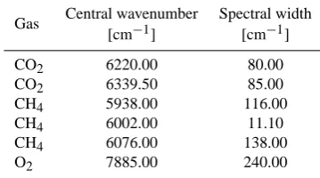
Table 1. Standard TCCON retrieval windows for CO2, CH4and O2.
Gas Central wavenumber Spectral width [cm−1] [cm−1]
CO2 6220.00 80.00
CO2 6339.50 85.00
CH4 5938.00 116.00
CH4 6002.00 11.10
CH4 6076.00 138.00
O2 7885.00 240.00
greenhouse gas instruments SCIAMACHY (Scanning Imag-ing Absorption Spectrometer for Atmospheric Cartography) onboard ENVISAT (Environmental Satellite), TANSO-FTS (Thermal And Near Infrared Sensor for Carbon Observation Fourier Transform Spectrometer) onboard GOSAT (Green-house Gases Observing Satellite) and OCO-2 (Orbiting Car-bon Observatory) are 7.0 cm−1, 0.2 cm−1and 0.3 cm−1, spectively. Since the individual spectral lines are not fully re-solved at these resolutions in the spectra recorded by these satellites, the retrieval requires a good knowledge of the background intensity and the underlying interfering gases.
Before using low resolution ground-based instruments in any network as an operational instrument, a validation and calibration procedure is required. The obvious choice to per-form such a validation/calibration campaign is to use high resolution TCCON instruments as a reference. Since our high resolution IFS 125 HR has been calibrated within the IMECC aircraft campaign it can serve as appropriate reference for the IFS 66. In this paper we present ground-based solar absorp-tion observaabsorp-tions of CO2and CH4using the small
commer-cial interferometer Bruker IFS 66 at its maximum possible resolution of 0.11 cm−1. The measurements have been per-formed in Bremen, Germany (53.1◦N, 8.8◦E) for nine days between winter 2009 and spring 2010. The results have been compared to observations performed by our high resolution TCCON instrument running at the same site in Bremen. Be-sides the direct comparison, the effect of the resolution on the retrieved columns has been investigated by truncating the high resolution spectra to a range of different resolutions be-tween 0.014 cm−1and 0.5 cm−1.
2 Instrumentation
solar tracker to the IFS 66, intercepting the sunlight to the high resolution instrument. This allows us to alternate mea-surements between the instruments. Spectra were recorded with the IFS 66 at a maximum resolution of 0.11 cm−1 and with the IFS 125 HR at 0.014 cm−1. In the IFS 125 HR the moving mirror is driven on a set of polished rails while the IFS 66 uses a frictionless air bearing. Both instruments use filter wheels to select the aperture. The aperture of the IFS 125 HR was set to 1.0 mm diameter, corresponding to a field of view of 0.0024 radians. For the IFS 66 we used an aperture of diameter 0.25 mm, resulting in a field of view of 0.0016 radians. While the diameter of the parallel light beam of the IFS 125 HR is 6.5 cm, the parallel beam of the IFS 66 is only 3.5 cm. Both instruments were equipped with CaF2 beamsplitters and indium gallium arsenide
(In-GaAs) IR-detectors, working at room temperature. Further-more, both instruments were purged with dry-air.
3 Measurements and analysis
Measurements from both instruments were recorded between November 2009 and April 2010 on nine clear days. The resulting solar absorption spectra were obtained alternately by changing the optical path of the sunlight between the instruments after each 30 min period. For the IFS 125 HR, two scans were averaged, while ten scans were averaged for the IFS 66. This leads to comparable observation times for each spectrum. For both instruments we used the commer-cial OPUS software package supplied by Bruker to record and transform the interferograms into spectra for later pro-cessing. To reduce the impact of source brightness fluctua-tions due to changes in the atmosphere, the retrieval strat-egy within TCCON is to normalize the DC recorded inter-ferograms with the low-pass filtered and smoothed signal (Keppel-Aleks, 2007). We did not apply this DC correction as the IFS 66 is not able to record a DC signal.
The analysis was performed using the least-squares algo-rithm GFIT, developed at NASA/JPL (Toon et al., 1992). The algorithm has been adapted for TCCON (Wunch et al., 2011). GFIT scales an assumed a-priori concentration profile until the simulated spectra best fit the observations by minimizing the RMS residual. The retrieved DMFs of CO2and CH4are
calculated by O2 as discussed in the introduction. So far it
is not possible to consider the detector noise in the GFIT re-trieval. In our analysis we used a beta-version of GFIT that has been modified to pre-adjust the stratospheric a-priori con-centration of CH4, by making use of the known correlation
between stratospheric CH4and HF. In the stratosphere HF is
a very stable trace gas. The tropospheric burden of HF can be neglected compared to the stratospheric one. Therefore, the total columns of HF, representing only the stratospheric burden, allow building a more realistic stratospheric a-priori profile of CH4(Washenfelder et al., 2003). This leads to
bet-ter spectral fits for CH4, as discussed later.
−0.2 −0.1 0 0.1 0.2 −5
0 5
a)
Wavenumbers [cm−1]
Transmittance [ ]
19.2°C 24.4°C 29.0°C
0 2 4 6 8
0.95 1
b)
OPD [cm]
Modulation efficiency [%]
19.2°C 24.4°C 29.0°C
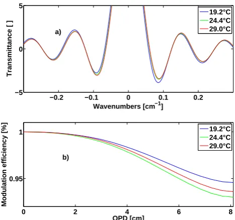
Fig. 1. Linefit evaluation with a HCl gas cell for different temper-atures. Panel (a) shows the ILS (the line is truncated to show the important part in more detail), (b) shows the modulation efficiency decreasing with the OPD.
4 Results
4.1 Alignment and stability
7 8 9 10 11 12 13 14 15 16 17 386
388 390 392 394 396 398 400
XCO
2(P)
UTC [h]
DMF [ppm]
IFS 66 IFS 125 HR
Fig. 2. Individual results for column-average dry-air mole fractions (DMF) of CO2, as measured by both instruments for 9 March 2010. The shown values are calculated by ratioing to the surface pressure rather than O2, as shown in Fig. 4. The SZAs vary from 78 degrees in the morning to 57 degrees at noon and 82 degrees in the after-noon.
ratio. A misalignment at the outgoing part of the FTS leads to a broadened ILS and a lowered resolution. A slope between the overlapping beams leads to an asymmetric ILS and a shift in wavelength. The lowering and the broadening of the ILS is not a major problem as we have enough intensity and high enough resolution. The shift in wavelength could be fitted, mainly the asymmetric ILS could become a serious problem. So far it is not possible to consider the measured ILS in the GFIT retrieval.
The ILS was retrieved with the “LINEFIT” program us-ing HCl lines from 5680 to 5800 cm−1 (Hase et al., 1999).
The IFS 125 HR typically gives a variation in the modulation efficiency of≤5 % over the full OPD. For the IFS 66, the modulation efficiency that has been measured directly after an alignment, increases linearly from 1.0 to 1.05 over the op-tical path difference of 8.1 cm. For this kind of opop-tical set up, using a 90◦ off-axis parabolic mirror in the interferometer, along with a frictionless air bearing for the movable mirror, a 5 % change in the modulation efficiency over the whole opti-cal path length is acceptable (A. K. Bruker, personal commu-nication, 2009). However, the alignment of the IFS 66 was found to be much more temperature sensitive than for the IFS 125 HR. Repeating the ILS measurements for conditions where the temperature of the whole laboratory was warmer by 10◦C resulted in a change in the modulation efficiency
of 2 %. We hence performed a test where we took cell mea-surements at different room temperatures, results are shown in Fig. 1.
The comparison for XCO2 by the IFS 66 with the
IFS 125 HR indicates good agreement between both instru-ments, independent of the alignment of the IFS 66. In com-parison, the results for XCH4 depend on the alignment, see
Tables 2 and 3. Tentatively, we assign this dependency to the combination of the least-squares fitting together with
0 0.5 1
Transmittance [ ]
b) IFS 125, OPD = 8.1 cm
−0.05 0 0.05
Residual [ ]
0 0.5 1
Transmittance [ ]
a) IFS 125, OPD = 64.3 cm
−0.05 0 0.05
Residual [ ]
0 0.5 1
Transmittance [ ]
c) IFS 66, OPD = 8.1 cm
measured spectrum calculated spectrum
6002.5 6003 6003.5 6004 −0.05
0 0.05
Wavenumbers [cm−1]
Residual [ ]
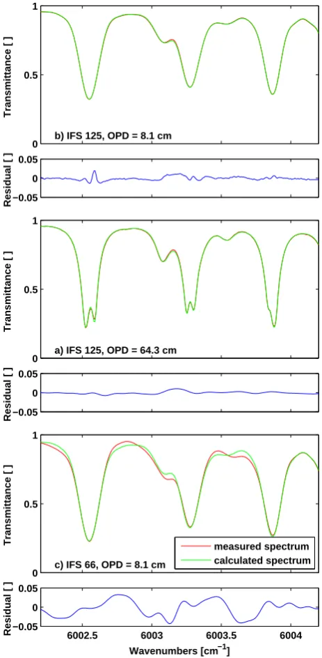
Fig. 3. Small part of a measured and simulated spectrum in the region of CH4. Panel (a) shows the high resolution spectrum of the IFS 125 HR at a resolution of 0.014 cm−1 (OPD = 64 cm), (b) is based on the same measurement, but the interferogram has been truncated to a resolution of 0.11 cm−1 (OPD = 8.1 cm), and (c) shows a spectrum measured by the IFS 66 at a resolution of 0.11 cm−1.
7 8 9 10 11 12 13 14 15 16 17 388
390 392 394 396 398 400
XCO2
UTC [h]
DMF [ppm]
IFS 66 IFS 125 HR
Fig. 4. Individual results for column-average dry-air mole fractions (DMF) of CO2, as measured by both instruments for 9 March 2010. 10 interferograms have been averaged for the IFS 66 for one data point, and 2 interferograms for the IFS 125 HR. With typical er-ror bars for single measurements as given by the retrieval software GFIT.
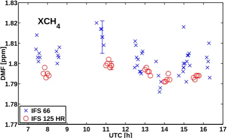
7 8 9 10 11 12 13 14 15 16 17 1.77
1.78 1.79 1.8 1.81 1.82 1.83
XCH
4
UTC [h]
DMF [ppm]
IFS 66 IFS 125 HR
Fig. 5. Individual results for column-average dry-air mole fractions (DMF) of CH4, as measured by both instruments for 9 March 2010. 10 interferograms have been averaged for the IFS 66 for one data point, and 2 interferograms for the IFS 125 HR. With typical er-ror bars for single measurements as given by the retrieval software GFIT.
case the quadratic dependency of the least-squares method yields wrong columns.
As an example, Fig. 3 shows part of the spectral fit in one CH4absorption window. Figure 3a shows the measurements
by the IFS 125 HR at a resolution of 0.014 cm−1 (64.3 cm OPD). Figure 3b shows the same spectrum as in Fig. 3a, but the interferogram has been truncated to 0.11 cm−1 (8.1 cm
OPD), corresponding to the resolution of the IFS 66. Fig-ure 3c shows the spectrum measFig-ured by the IFS 66 at a res-olution of 0.11 cm−1(8.1 cm OPD). The residuals of Fig. 3c have systematic deviations at the absorption lines, which we attribute to non-optimal alignment of the interferometer. Our measurements show that the retrieved values are acceptable for this instrument despite the asymmetric fit as shown in Fig. 3c.
23−Nov−2009 12−Jan−2010 03−Mar−2010 22−Apr−2010 384
388 392 396
XCO2
Date
DMF [ppm]
IFS 66 IFS 125 HR
Fig. 6. Daily averages of XCO2, as measured by the IFS 66 and the IFS 125 HR. The daily means are calculated from single measure-ments as a weighted mean, weighted to the reciprocal of their error variance. As example typical error bars of oneσ are shown.
23−Nov−2009 12−Jan−2010 03−Mar−2010 22−Apr−2010 1.74
1.76 1.78 1.8 1.82
XCH 4
Date
DMF [ppm]
IFS 66 IFS 125 HR
Fig. 7. Daily averages of XCH4, as measured by the IFS 66 and the IFS 125 HR. The statistics are calculated as described for XCO2in Fig. 6.
4.2 Precision and comparability
Results for individual measurements of XCO2and XCH4are
shown in Figs. 4 and 5. The error bars indicate the typical uncertainty for single measurements as given by the retrieval software GFIT. The shown day is selected as it covers a large variation of solar zenith angles (SZA) from 78 degrees in the morning to 57 degrees at noon and 82 degrees in the after-noon. The measurements of XCO2and XCH4show that there
is not a significant dependency on SZAs. For the IFS 66, we obtained a precision of 0.32 % (1.2 ppm) for CO2and 0.41 %
for CH4(7.3 ppb). For comparison, the network wide
preci-sion of the IFS 125 HR was found to be 0.25 % (1.0 ppm) for CO2and 0.22 % (3.9 ppb) for CH4, in agreement with Wunch
Table 2. Daily means of XCO2for nine measuring days. The daily means are calculated from single measurements as a weighted mean, weighted to the reciprocal of their error variance. As an estimation for the error of the daily means the standard deviation,σ, is given. The differences of the daily means are given in percent while the averages of differences are calculated from the absolute values.
XCO2IFS-125 HR 1σ XCO2IFS-66 1σ Difference
Day [ppm] [ppm] [ppm] [ppm] [%]
20 November 2009 385.00 0.48 385.27 1.05 0.07
1 December 2009 387.53 0.25 387.56 1.13 0.01
28 December 2009 388.59 2.98 388.55 1.90 -0.01
22 January 2010 389.07 0.60 388.36 0.76 -0.18
Average before alignment 387.55 1.08 387.44 1.21 0.07
4 March 2010 392.20 2.17 392.55 1.63 0.09
5 March 2010 392.02 0.18 391.63 1.17 -0.10
9 March 2010 392.44 1.61 392.69 1.38 0.06
12 April 2010 391.87 0.32 391.32 0.90 -0.14
15 April 2010 393.00 0.25 392.48 1.17 -0.13
Average after alignment 392.31 0.91 392.13 1.25 0.11
Table 3. Daily means of XCH4for nine measuring days. The statistics are calculated as described for XCO2in Table 2. In the last column an offset of 0.47 % is subtracted from the daily means measured by the IFS-66, then the difference is calculated and given in percent. Again, the averages of differences are calculated from the absolute values.
XCH4IFS-125 HR σ XCH4IFS-66 σ Difference Diff.-offset
Day [ppm] [×10−2ppm] [ppm] [×10−2ppm] [%] [%]
20 November 2009 1.776 0.52 1.746 1.29 -1.69 -2.15
1 December 2009 1.785 0.17 1,771 1.14 -0.78 -1.25
28 December 2009 1.798 0.73 1.770 0.53 -1.56 -2.02
22 January 2010 1.803 0.45 1.792 0.57 -0.61 -1.08
Average before alignment 1.791 0.47 1.770 0.88 1.16 1.62
4 March 2010 1.777 1.11 1.788 0.79 0.62 0.15
5 March 2010 1.785 0.18 1.796 0.79 0.62 0.14
9 March 2010 1.795 0.39 1.801 0.71 0.33 -0.14
12 April 2010 1.768 0.20 1.773 0.83 0.28 -0.19
15 April 2010 1.794 0.07 1.803 0.51 0.50 0.03
Average after alignment 1.784 0.39 1.792 0.73 0.47 0.13
Comparing the daily means from both instruments gives an average deviation of 0.09 % or 0.35 ppm for XCO2which
is within the precision of both instruments (Fig. 6). Daily means for XCH4 are shown in Fig. 7. For XCH4 the
re-sults from the IFS 66 are lower by 0.47 % compared to the IFS 125 HR. The offset is constant and larger than the preci-sion. After subtracting this offset, the average deviations of both instruments is 0.13 %, in agreement with the precision of both instruments.
Till the 22 January 2010, the IFS 66 was not well aligned, so the effect of an improperly aligned instrument on the re-sulting XCO2and XCH4could be tested by comparing the
results.
While XCO2is only slightly affected by a bad alignment,
the deviations for XCH4 increase by a factor of three, as
given in Tables 2 and 3.
Evaluating the total columns of CO2and CH4shows
sim-ilar results. O2and CO2agree within the error bars, expect
for very high SZAs in the early morning and late evening. In the ratio this deviation is canceled out. Figure 2 shows the retrieved XCO2calculated by ratioing to the surface pressure
column rather than measured O2as is shown in Fig. 4,
show-ing the effect of the ratioshow-ing to O2. CH4differs in the same
way as XCH4with additional errors for very high SZAs. The
difference of CO2and CH4as measured by both instruments
8 10 12 14 16 18 384
386 388 390 392 394
XCO
2
UTC [h]
DMF [ppm]
OPD = 8.11 cm OPD = 64.29 cm
Fig. 8. Retrieved XCO2from observations by the high resolution instrument IFS 125 HR for the 16 April 2009. The red symbols cor-respond to the high resolution of 0.014 cm−1, the blue symbols to a resolution of 0.11 cm−1.
8 10 12 14 16 18
1.76 1.78 1.8 1.82
XCH
4
UTC [h]
DMF [ppm]
OPD = 8.11 cm OPD = 64.29 cm
Fig. 9. Retrieved XCH4from observations by the high resolution instrument IFS 125 HR for the 16 April 2009. The red symbols cor-respond to the high resolution of 0.014 cm−1, the blue symbols to a resolution of 0.11 cm−1.
4.3 Influence of resolution
When comparing XCH4obtained from both instruments, we
attribute the offset of 0.47 % to a combination of improper a-priori profiles, erroneous spectroscopic data, and / or incor-rect assumptions in the pT-profile in the retrieval. The residu-als in Fig. 3 indicate a perfect fit. We speculate that non-ideal choice of input parameters for the least-squares fitting procedure have different effects for the low resolution spec-tra compared to the high resolution ones. In order to test the effect of the resolution, we truncated the high resolution in-terferograms of the IFS 125 HR to a resolution of 0.11 cm−1, the resolution used by the IFS 66. The results are shown in Figs. 8 and 9. While XCO2shows almost no dependence on
the resolution (0.02 %), for XCH4a constant offset of 0.26 %
can be observed. The remaining 0.21 % are within the uncer-tainties for XCH4and we get agreement with our estimation
given above.
4.516 4.52 4.524 4.528 4.532
0.1% a) O2
[*10
2
4 molec cm
−
2]
8.275 8.28 8.285 8.29 8.295 8.3
0.1% c) CO
2
OPD [cm]
[*10
2
1 molec cm
−
2]
CO2 6220−window CO
2 6339−window
3.76 3.78 3.8 3.82
0.1% b) CH
4
[*10
1
9 molec cm
−
2]
CH4 5938−window CH4 6002−window CH
4 6076−window
0 10 20 30 40 50 60 70 3.76
3.78 3.8 3.82
0.1% d) CH
4
OPD [cm]
[*10
1
9 molec cm
−
2]
CH4 5938−window, shifted vmr CH4 6002−window, shifted vmr CH
4 6076−window, shifted vmr
Fig. 10. Retrieved O2, CO2 and CH4 total columns from the IFS 125 HR, by truncating the interferograms to different optical path differences. For CO2and CH4the different retrieval windows are shown. For CH4the initial a-priori profile has been shifted ver-tically by−4 km. The shown bars give a percentage scale.
3.95 4 4.05 4.1 4.15
1% a) H2O
[*10
2
2 molec cm
−
2]
from CH4 5938−window from CH4 6002−window from CH4 6076−window
388 388.2 388.4 388.6
0.1% c) XCO
2
OPD [cm]
DMF [ppm]
1.794 1.796 1.798 1.8
0.1% b) XCH4
DMF [ppm]
0 10 20 30 40 50 60 70 1.792
1.794 1.796 1.798
0.1% d) XCH
4
OPD [cm]
DMF [ppm]
XCH4, shifted vmr
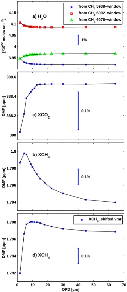
Fig. 11. Retrieved H2O, XCO2 and XCH4 from the IFS 125 HR, H2O is taken from the different retrieval windows of CH4. For XCH4 the initial a-priori profile has been shifted vertically by
−4 km. The shown bars give a percentage scale.
measured on 16 April 2009. Shown is the daily mean. For reference, the variability in percent for each compound is given as a bar in the figure. The dependence on the OPD in-creases with decreasing OPD. Down to an OPD of 6 cm (res-olution of 0.15 cm−1), the O2and CO2columns show only
a weak dependency of 0.02 %. For CH4columns, the
vari-ation is much larger, between 0.05 % and 0.3 %, depending on the spectral band analyzed. The corresponding results for
XCO2, XCH4and the most important interfering gas, H2O,
are also shown. The dependency for H2O is about 0.1 %. As
there are H2O lines in the window where CH4 is retrieved
(5938 cm−1, 6002 cm−1and 6076 cm−1), for low resolution spectra the lines cannot be separated.
These simulations for XCO2and XCH4are in agreement
with the results from the comparison of both instruments, as shown in Figs. 4 and 5. While the CO2 total columns for
both instruments agree within the precision, for CH4, a
con-stant bias of 0.26 % was found. It has to be mentioned that standard TCCON measurements are made with an OPD of 40 cm and are not significantly affected.
In order to investigate the dependency of CH4on the OPD
in more detail, we shifted the whole a-priori VMR profile of CH4down by 4 km, and repeated the resolution-dependant
sensitivity study shown in Figs. 10c and 11c. The results are displayed in Figs. 10d and 11d. The simulations show that the dependency of the resolution on the CH4 total
col-umn is less. Furthermore, the dependency of the windows at 6002 cm−1and 6076 cm−1nearly compensate each other. We tried also other vertical shift amounts, i.e. 2, 4, 6 and 8 km, with 4 km yielding the “optimum” result. That is, 4 km yielded the smallest dependency on the OPD. A downshift-ing of the a-priori VMR by 4 km is certainly not realistic, but our results might indicate that the a priori and/or the spec-tral data of CH4 are erroneous. For completeness, we have
repeated the simulations for CO2and O2 but the results do
not depend on shifting the a priori up and down (not shown), which is not surprising, as the volume mixing ratio of both trace gases show only weak variability with altitude.
Our study indicates that the retrieved columns depend on the resolution, especially if the assumed a-priori VMR pro-file is not perfect. However, it must be mentioned that within TCCON, the retrieval strategy applied so far is profile scal-ing. When applying a complete profile retrieval algorithm, the OPD dependency will look different. Differences for CH4
total columns depending on the retrieval algorithm have al-ready been observed by Petersen et al. (2010), who compared profile scaling with the optimal estimation approach for trop-ical spectra from Suriname.
5 Summary and conclusion
The precision for the low resolution instrument was found to be 0.32 % for XCO2 (1.2 ppm) and 0.41 % (7.3 ppb) for
XCH4. For comparable measurement times, the precision of
the IFS 66 is lower compared to the IFS 125 HR, which can be explained by the lower light throughput of the IFS 66. The comparison of both instruments gives good agreement, devi-ation of daily means is below 0.2 % (0.6 ppm) for XCO2. For
XCH4a constant offset of 0.47 % has been observed. After
subtracting the constant offset, the average deviation between the instruments was also of the order of 0.2 % (4 ppb). Trun-cating the high resolution interferograms of the IFS 125 HR so the resolution is equivalent to the resolution of the IFS 66 gives an offset of 0.26 %, which partly explains the measured offset of the IFS 66 for CH4. The ILS of the low resolution
in-strument was found to depend on the temperature. While the results for XCO2do not depend on the temperature and
align-ment, for XCH4 the precision and comparability require a
well aligned instrument. Overall we can conclude that XCO2
can be measured with a low resolution FTS instrument with sufficient precision and accuracy, however, for XCH4the
re-sults depend on the alignment.
Acknowledgements. We acknowledge the support by the European Commission of the Integrated Project InGOS (Integrated non-CO2 Greenhouse gas Observation System) within the 7th Framework Program. We acknowledge the ESA GHG CCI (European Space Agency Green House Gas Climate Change Initiative) project. We thank Nick Deutscher for his comments on the manuscript. This work was financially supported by the University of Bremen and the Senate of Bremen.
Edited by: I. Aben
References
Deutscher, N. M., Griffith, D. W. T., Bryant, G. W., Wennberg, P. O., Toon, G. C., Washenfelder, R. A., Keppel-Aleks, G., Wunch, D., Yavin, Y., Allen, N. T., Blavier, J.-F., Jim´enez, R., Daube, B. C., Bright, A. V., Matross, D. M., Wofsy, S. C., and Park, S.: Total column CO2measurements at Darwin, Australia – site de-scription and calibration against in situ aircraft profiles, Atmos. Meas. Tech., 3, 947–958, doi:10.5194/amt-3-947-2010, 2010. Hase, F., Blumenstock, T., and Paton-Walsh, C.: Analysis of the
instrumental line shape of high-resolution Fourier transform IR spectrometers with gas cell measurements and new retrieval soft-ware, Appl. Optics, 38, 3417–3422, doi:10.1364/AO.38.003417, 1999.
Keppel-Aleks, G., Toon, G. C., Wennberg, P. O., and Deutscher, N. M.: Reducing the impact of source brightness fluctuations on spectra obtained by Fourier-transform spectrometry, Appl. Op-tics, 46, 4774–4779, 2007.
Messerschmidt, J., Macatangay, R., Notholt, J., Petri, C., Warneke, T., and Weinzierl, C.: Side by side measurements of CO2 by
ground-based Fourier transform spectrometry (FTS), Tellus B, 62, 749–758, 2010.
Messerschmidt, J., Geibel, M. C., Blumenstock, T., Chen, H., Deutscher, N. M., Engel, A., Feist, D. G., Gerbig, C., Gisi, M., Hase, F., Katrynski, K., Kolle, O., Lavriˇc, J. V., Notholt, J., Palm, M., Ramonet, M., Rettinger, M., Schmidt, M., Suss-mann, R., Toon, G. C., Truong, F., Warneke, T., Wennberg, P. O., Wunch, D., and Xueref-Remy, I.: Calibration of TCCON column-averaged CO2: the first aircraft campaign over Euro-pean TCCON sites, Atmos. Chem. Phys., 11, 10765–10777, doi:10.5194/acp-11-10765-2011, 2011
Petersen, A. K., Warneke, T., Frankenberg, C., Bergamaschi, P., Gerbig, C., Notholt, J., Buchwitz, M., Schneising, O., and Schrems, O.: First ground-based FTIR observations of methane in the inner tropics over several years, Atmos. Chem. Phys., 10, 7231–7239, doi:10.5194/acp-10-7231-2010, 2010.
Toon, G. C., Farmer, C. B., Schaper, P. W., Lowes, L. L., and Nor-ton, R. H.: Composition measurements of the 1989 arctic winter stratosphere by airborne infrared solar absorption spectroscopy, J. Geophys. Res., 97, 7939–7961, doi:10.1029/91JD03114, 1992.
Warneke, T., Yang, Z., Olsen, S., Korner, S., Notholt, J., Toon, G. C., Velazco, V., Schulz, A., and Schrems, O.: Seasonal and latitudinal variations of column averaged volume-mixing ra-tios of atmospheric CO2, Geophys. Res. Lett., 32, L03808, doi:10.1029/2004GL021597, 2005.
Washenfelder, R. A., Wennberg, P. O., and Toon, G. C.: Tropospheric methane retrieved from ground-based near-IR solar absorption spectra, J. Geophys. Res., 30, 2226, doi:10.1029/2003GL017969, 2003.
Washenfelder, R., Toon, G., Blavier, J., Yang, Z., Allen, N., Wennberg, P., Vay, S., Matross, D., and Daube, B.: Carbon diox-ide column abundances at the Wisconsin Tall Tower site, J. Geo-phys. Res., 111, D22305, doi:10.1029/2006JD007154, 2006. Wunch, D., Toon, G. C., Wennberg, P. O., Wofsy, S. C., Stephens,
B. B., Fischer, M. L., Uchino, O., Abshire, J. B., Bernath, P., Bi-raud, S. C., Blavier, J.-F. L., Boone, C., Bowman, K. P., Browell, E. V., Campos, T., Connor, B. J., Daube, B. C., Deutscher, N. M., Diao, M., Elkins, J. W., Gerbig, C., Gottlieb, E., Griffith, D. W. T., Hurst, D. F., Jim´enez, R., Keppel-Aleks, G., Kort, E. A., Macatangay, R., Machida, T., Matsueda, H., Moore, F., Morino, I., Park, S., Robinson, J., Roehl, C. M., Sawa, Y., Sherlock, V., Sweeney, C., Tanaka, T., and Zondlo, M. A.: Calibration of the Total Carbon Column Observing Network using aircraft pro-file data, Atmos. Meas. Tech., 3, 1351–1362, doi:10.5194/amt-3-1351-2010, 2010.
Wunch, D., Toon, G. C., Blavier, J.-F. L., Washenfelder, R. A., Notholt, J., Connor, B., Griffith, D., and Wennberg, P. O.: The Total Carbon Column Observing Network (TCCON), Philos. T. R. Soc. A., 369, 1943, doi:10.1098/rsta.2010.0240, 2011. Yang, Z. H., Toon, G. C., Margolis, J. S., and Wennberg, P. O.:
At-mospheric CO2retrieved from ground-based near IR solar spec-tra, Geophys. Res. Lett., 29, 1339, doi:10.1029/2001GL014537, 2002.