www.atmos-meas-tech.net/8/4133/2015/ doi:10.5194/amt-8-4133-2015
© Author(s) 2015. CC Attribution 3.0 License.
Optimization of the GSFC TROPOZ DIAL retrieval using synthetic
lidar returns and ozonesondes – Part 1: Algorithm validation
J. T. Sullivan1,4,a, T. J. McGee1, T. Leblanc2, G. K. Sumnicht3, and L. W. Twigg3
1Atmospheric Chemistry and Dynamics Branch, NASA Goddard Space Flight Center, Greenbelt, MD, USA 2California Institute of Technology, Jet Propulsion Laboratory, Wrightwood, CA, USA
3Science Systems and Applications Inc., Lanham, MD, USA 4Oak Ridge Associated Universities (ORAU), Oak Ridge, TN, USA
aformerly at: Department of Atmospheric Physics, University of Maryland, Baltimore County (UMBC) and Joint Center for Earth Systems Technology (JCET), Baltimore, MD, USA
Correspondence to: J. T. Sullivan ([email protected])
Received: 11 February 2015 – Published in Atmos. Meas. Tech. Discuss.: 28 April 2015 Revised: 28 August 2015 – Accepted: 16 September 2015 – Published: 9 October 2015
Abstract. The main purpose of the NASA Goddard Space Flight Center TROPospheric OZone DIfferential Absorp-tion Lidar (GSFC TROPOZ DIAL) is to measure the ver-tical distribution of tropospheric ozone for science investi-gations. Because of the important health and climate im-pacts of tropospheric ozone, it is imperative to quantify back-ground photochemical ozone concentrations and ozone lay-ers aloft, especially during air quality episodes. For these rea-sons, this paper addresses the necessary procedures to vali-date the TROPOZ retrieval algorithm and confirm that it is properly representing ozone concentrations. This paper is fo-cused on ensuring the TROPOZ algorithm is properly quanti-fying ozone concentrations, and a following paper will focus on a systematic uncertainty analysis.
This methodology begins by simulating synthetic lidar re-turns from actual TROPOZ lidar return signals in combina-tion with a known ozone profile. From these synthetic sig-nals, it is possible to explicitly determine retrieval algorithm biases from the known profile. This was then systematically performed to identify any areas that need refinement for a new operational version of the TROPOZ retrieval algorithm. One immediate outcome of this exercise was that a bin reg-istration error in the correction for detector saturation within the original retrieval was discovered and was subsequently corrected for. Another noticeable outcome was that the verti-cal smoothing in the retrieval algorithm was upgraded from a constant vertical resolution to a variable vertical resolu-tion to yield a statistical uncertainty of <10 %. This new
and optimized vertical-resolution scheme retains the ability to resolve fluctuations in the known ozone profile, but it now allows near-field signals to be more appropriately smoothed. With these revisions to the previous TROPOZ retrieval, the optimized TROPOZ retrieval algorithm (TROPOZopt) has been effective in retrieving nearly 200 m lower to the surface. Also, as compared to the previous version of the retrieval, the TROPOZopthad an overall mean improvement of 3.5 %, and large improvements (upwards of 10–15 % as compared to the previous algorithm) were apparent between 4.5 and 9 km. Fi-nally, to ensure the TROPOZoptretrieval algorithm is robust enough to handle actual lidar return signals, a comparison is shown between four nearby ozonesonde measurements. The ozonesondes are mostly within the TROPOZoptretrieval un-certainty bars, which implies that this exercise was quite suc-cessful.
1 Introduction
from a 13 m transportable trailer since fall of 2013. Many of the instrument specifications and initial TROPOZ retrieval algorithm, which are the baseline retrieval for this paper, can be found in Sullivan et al. (2014). This instrument has been developed as part of the ground-based Tropospheric Ozone Lidar NETwork (TOLNet), which currently consists of five stations across the United States (http://www-air. larc.nasa.gov/missions/TOLNet/). Because this network con-sists of five different ozone lidar systems, it is important that retrievals for each site be independently validated and compared to provide accurate information for future science campaigns. In May 2014, an intercomparison between the TROPOZ and the Langley Mobile Ozone Lidar (LMOL, Pli-utau and De Young, 2013) was performed in which no biases were apparent as compared to ozonesonde profiles when re-trievals were performed with adequate signal (Sullivan et al., 2015). Additionally, the TROPOZ and NOAA TOPAZ (Tun-able Optical Profiler for Aerosol and oZone lidar, Alvarez et al., 2011) were operated simultaneously for several days in July 2014, and a detailed intercomparison is currently be-ing performed.
The most common method for validation of ozone li-dars is sending a balloon-borne electrochemical concentra-tion cell (ECC) instrument through the atmosphere, and it has generally been used as the community validation stan-dard (Thompson et al., 2003). Although launching ECC son-des may be a useful validation tool, the instantaneous ECC measurement may be transported a non-negligible distance away from the ozone lidar resulting in a large difference in air mass. For these reasons, this paper describes the useful-ness of utilizing synthetic lidar return signals that are com-puted using a known ozone profile as an independent vali-dation method in addition to nearby ozonesonde launches. This process also prevents errors in the retrieval process from invalidating quality data. Using simulated lidar data instead of an ozonesonde profile is advantageous because by vary-ing parameters in the modeled return signal, it is possible to explicitly determine both the source and the magnitude of various biases in the retrieval from the original ozone profile (Leblanc et al., 1998; Keckhut et al., 2004a).
This paper addresses the necessary procedures to validate the optimized TROPOZ retrieval algorithm (TROPOZopt) as compared to the previous Sullivan et al. (2014) algorithm and to confirm that it is properly representing ozone concentra-tions. A following paper will further focus on a systematic uncertainty analysis with the same proposed methodology. The parameters investigated within this paper are the correc-tions that occur naturally from spectral properties of trace gases within the atmosphere (including ozone) and limita-tions of the hardware used to resolve the atmosphere. The numerical derivative is analyzed first to show that it is being performed correctly. Because of naturally varying tempera-tures in the atmosphere, the temperature dependences of the ozone absorption cross sections are also analyzed. The DIAL measurement involves two wavelengths, and a correction for
the differential scattering properties of the Rayleigh atmo-sphere is also investigated. Additionally, because the detec-tors reach a regime where they cannot account for the proper amount of return signal, a detector saturation (or pulse pile-up) correction is described and analyzed. Vertical resolution is also examined as it can be a controlling factor in repre-senting the correct ozone mixing ratio profile, especially in the upper free troposphere with a decreasing signal to noise ratio (SNR). All of these corrections and refinements were implemented into the new TROPOZopt retrieval algorithm, and the final section of this paper shows a comparison with good agreement with actual ozone retrievals and four nearby ozonesonde profiles.
2 Synthetic lidar returns and initial retrieval
In order to validate the GSFC TROPOZ DIAL retrieval al-gorithm, synthetic lidar return signals have been generated using physical parameters of the lidar system, climatological data, and a known ozone profile. The purpose of generating these synthetic signals is to investigate various parts of the re-trieval algorithm with the ability to turn varying effects, such as ambient background radiation, saturation effects, or spec-tral properties of the atmosphere, on or off. With the ability to vary these effects and decompose the synthetic signals, the TROPOZ retrieval algorithm can be tested in a rigorous manner in order to identify any uncertainty and bias with the original ozone profile.
The synthetic signals were computed using a known at-mospheric state produced by the empirical model MSISE-90 (Hedin, 1991) between the ground and the thermosphere. The model computes a temperature profile, and profiles of the main atmospheric constituents’ number densities includ-ing N2, O2, and Ar for a given day of year and time of day. Additionally, the atmospheric state includes an ozone num-ber density profile computed from a combination of clima-tologies taken from the UK Universities Global Atmospheric Modelling Programme (UGAMP; Thuburn, 1992) and from the UARS Reference Atmosphere Project.
The simulated lidar return signals are calculated as
P (i, k)=PL(i)η(i, k)Na(k)
(z(k)−zL)2
β(i, k)τO3(i, k)τM(i, k), (1)
where
τO3 =e −Pk
k0 =0NO3(k)(σO3↑(i,k0)+σO3↓(i,k0))δz, (2)
τM=e− Pk
k0 =0Na(k)(σM↑(i,k0)+σM↓(i,k0))δz, (3) and theiandkindices denote the “on” and “off” DIAL wave-length and altitude, respectively. P is the total number of photons collected at each wavelength,ηis the optical effi-ciency of the receiving channel,Nais the air number density,
layer is denoted asβ, which is currently only from molecular scattering. The optical thickness from the test ozone profile,
τO3, and from the Rayleigh atmosphere,τM, are integrated
along the outgoing beam path (↑)and integrated along the returning beam path(↓)between the lidar and the scattering altitude. The test ozone number density profile is NO3, the
ozone absorption cross sections are σO3 and the molecular
scattering cross sections areσM.
After the atmospheric signals have been generated, the ef-fects of saturation of the detectors and background noise in all channels are computed as
S(i, k)=(i) P (i, k)
1+P (i, k)Td(i)+Pb(i, k), (4)
where represents the amplification factor or efficiency of the data recorder system,Tdis the theoretical dead time cor-rection andPbincludes background noise in all channels to account for sky light and electronic noise.
These hardware and atmospheric effects are generated based on various physical components of the TROPOZ li-dar system described in Sullivan et al. (2014). Examples of these are the field of view (FOV) of each of the detectors, fil-ter bandwidths, the altitudes at which the signals were gated, and the assumption that the signal can be corrected using a nonparalyzable dead time correction for the photomultiplier tubes (PMTs). The saturation correction is based on the laser repetition rate and the photon counting rate of the data acqui-sition system. The synthetic signals were also modeled from the standard meteorological atmosphere from the TROPOZ site elevation, latitude, and longitude. In order to properly represent the magnitudes of the synthetic signal, cloud-free, nighttime data are used to simulate realistic return signal lev-els. Nighttime conditions, where there is naturally a lower level of background noise, allow for a larger vertical range of validation. These acquired signals are then temporally aver-aged for 10 min for comparison with the analysis and uncer-tainty discussion previously reported in Sullivan et al. (2014).
3 The DIAL equation
The simulated lidar return signals are not recorded as con-tinuous functions, but rather as values in discrete range bins,
1z, at the “on” and “off” DIAL wavelengths. It is then possi-ble to write the discrete DIAL equation (Megie et al., 1985) in terms of the range bins specified as
NO3(z)=
1 21σO31z
ln(Soff(z+1z) Soff(z)
Son(z)
Son(r+1z)
−C)−D, (5) where
C=βoff(z+1z)
βoff(z)
βon(z)
βon(z+1z)
) (6)
0 50 100 150 200 250 0
1.5 3 4.5 6 7.5 9
Ozone MR [ppbv]
Altitude [km AGL]
TROPOZ Truth
−045−30−15 0 15 30 45 1.5
3 4.5 6 7.5 9
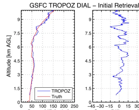
Ozone Difference [%] GSFC TROPOZ DIAL − Initial Retrieval
Figure 1. The left panel shows the initial retrieved ozone concentra-tion from the TROPOZ algorithm described in Sullivan et al. (2014) as compared to the known ozone profile used in the simulated lidar return signals. The right panel shows the percent difference from the known profile and retrieved profile.
and with negligible amounts of aerosols and additional inter-fering gases,
D=1αM
1σO3
. (7)
For these equations,NO3 is the ozone number density and 1σO3 is the difference in corresponding ozone absorption
cross sections taken at the two DIAL wavelengths. The power, atmospheric backscatter coefficient, and atmospheric extinction received from rangezat either the “on” or “off” wavelength are denoted asP,βandαrespectively. The term,
1αM, is the difference in the Rayleigh extinction properties of the atmosphere between the two DIAL wavelengths.
The DIAL Eq. (5) is of great interest, and it is of great interest because it lends itself to a self-calibrating technique that can determine the number density of ozone with only the known ozone absorption cross sections and the power returned at each wavelength. The power returned back to the detector is a convolution of backscattered photons from the molecular atmosphere and ambient background sky ra-diation. Therefore,Poff and Pon are actually comprised of
Poff+PbandPon+Pb, wherePbis the background radiation at the respected DIAL wavelengths.
as-sumed Rayleigh phase function. The implementation of this correction is discussed in a later section of this paper. Al-though aerosols are not simulated explicitly for this analysis, the aerosol correction discussed in Sullivan et al. (2014) is utilized when comparing the optimized retrieval to actual li-dar return signals.
After the TROPOZ retrieval was performed on the syn-thetic return signals, a final ozone concentration profile was computed. It is then possible to truly compare the final ozone profile to the truth profile originally used to produce the sim-ulated synthetic signals. This is not entirely possible with co-located launches of ozonesondes and shows the advantage of using simulated data as an independent validation source. In-vestigation of any differences between the TROPOZ retrieval and the true profile can lead to the identification of quantifi-able algorithmic biases.
Figure 1 shows the initial TROPOZ retrieval (Sullivan et al., 2014) and its associated ozone differences from the modeled truth profile (red) from 675 m to 10 km. This is a composite profile which represents two different signal pairs from 675 m to 2.75 km and from 2.75 m to 10 km. The def-inition of the relative percent difference used for Fig. 1, as well as throughout this paper, is
1NO3(%)=
TROPOZNO3−ModelNO3
ModelNO3
×100. (8)
This retrieval has been performed with a constant 375 m ver-tical resolution below 2.75 km and a 750 m verver-tical resolu-tion above 2.75 km. For the region above 4.5 km, this fixed vertical resolution starts to yield large ozone differences near 15 %, which can certainly be improved upon and are most likely directly attributed to smoothing effects. Also, near the bottom of the profile and near the join region (2.75–3 km), there is a comparably large ozone difference which will be discussed in a later section of this work. Although the dif-ferences between the initial and final ozone profiles in Fig. 1 are mostly within 15 %, there are still underlying biases that may be decreased, and this is the motivation for the following sections of this paper.
3.1 Numerical derivative
The first step in ensuring that the DIAL retrieval algorithm is accurate is to confirm that the derivative of the natural loga-rithm of the ratio of backscattered laser powers from Eq. (5) is correctly calculated. For this reason, a synthetic lidar re-turn signal is simulated to emphasize the use of the numer-ical derivative. The statistnumer-ical and background noise, satu-ration correction, and Rayleigh correction were all removed for this simulation and constant ozone absorption cross sec-tions were used with values ofσO3299=4.200e
−23m2and
σO3289=1.542e−22m2(Malicet et al., 1995).
The finite impulse response (FIR) Savitzky–Golay (SG) differentiation filter (Savitzky and Golay, 1964) used for the
0 50 100 150 200 250
0 1.5 3 4.5 6 7.5 9
Ozone MR [ppbv]
Altitude [km AGL]
Corr. Truth
−03 −2 −1 0 1 2 3 1.5
3 4.5 6 7.5 9
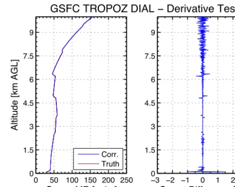
Ozone Difference [%] GSFC TROPOZ DIAL − Derivative Test
Figure 2. The left panel shows the initial retrieved ozone concen-tration from the TROPOZ algorithm using the Savitzky–Golay dif-ferentiation filter for the numerical derivative as compared to the known ozone profile used in the simulated lidar return signals. The right panel shows the percent difference from the known profile and retrieved profile.
numerical derivative is the same described in Sullivan et al. (2014). The advantage of using the SG filter is that the fi-nal vertical resolution of the retrieved ozone can be easily determined using the full width at half maximum (FWHM) of the steady-state SG filter coefficients associated with the filter window size. To emphasize the possible biases from the numerical derivative, the retrieval is done with a minimal three-point smoothing.
The results for using the SG filter are shown in Fig. 2, where the left panel shows the final retrieved ozone mix-ing ratio from the corrected TROPOZ numerical derivative (blue) as compared to the known ozone profile (red) used in the simulated lidar return signal. Both profiles are in the fig-ure but are directly overtop of each other, implying the nu-merical derivative is being properly computed in the retrieval algorithm. The right panel shows the negligible percent dif-ference between the known profile and retrieved profile, and this will continue to be used in the new operational version of the TROPOZoptozone retrieval.
3.2 Temperature dependence of the ozone absorption cross section
Due to the known temperature dependence of the ozone absorption cross section, it is necessary to get an accurate atmospheric temperature profile, either from a co-located radiosonde launch or from a standard model atmosphere. Ozone absorption cross sections were utilized from Malicet et al. (1995) because of the adequate coverage of standard tropospheric temperatures at the DIAL wavelengths. The
nec-0 50 100 150 200 250 0
1.5 3 4.5 6 7.5 9
Ozone MR [ppbv]
Altitude [km AGL]
Truth Constant Spline Linear Nearest Cubic
−3 −2 −1 0 1 2 3 0
1.5 3 4.5 6 7.5 9
Ozone Difference [%] GSFC TROPOZ DIAL − Temp. Dependence
Figure 3. The left panel shows the retrieved ozone mixing ratio from the varying TROPOZ interpolations of the temperature de-pendence of ozone absorption cross sections as compared to the known ozone profile used in the simulated lidar return signal.The right panel shows the percent difference from the known profile and retrieved profile.
essary to characterize resulting ozone differences from this temperature dependence. Because the ozone absorption tem-perature dependence is not known continuously but rather at discrete temperatures, various interpolations have been in-vestigated and are all shown.
In the left panel of Fig. 3, ozone mixing ratios are retrieved using the constant ozone absorption cross sec-tions ofσO3299=4.200e
−23m2andσ
O3289=1.542e −22m2, but with varying temperature interpolations (Malicet et al., 1995). The statistical and background noise, saturation cor-rection and Rayleigh corcor-rection were all removed for this simulation. One profile corresponds to constant values of
1σO3, and additional profiles use a different interpolation
of the ozone absorption cross sections. Although the final mixing ratios look very similar for each temperature inter-polation, the right panel of Fig. 3 shows subtle differences between the various interpolation schemes (Boor, 1978). For spline fitting, the interpolated value at a query point is based on a cubic interpolation of the values using not-a-knot condi-tions at neighboring grid points. For linear and cubic fitting, the interpolated value at a query point is based on linear and cubic interpolation of the values. For nearest fitting, the in-terpolated value at a query point is the value at the nearest sample grid point.
Regardless of the interpolation used for the synthetic re-turn, the final ozone differences are all mostly within 2 % of the known ozone profile. The blue line, representing a con-stant temperature value, emphasizes the importance of cor-recting the TROPOZ retrieval algorithm for temperature, es-pecially in the first few kilometers of the troposphere. The
0 50 100 150 200 250 0
1.5 3 4.5 6 7.5 9
Ozone MR [ppbv]
Altitude [km AGL]
Corr. Uncorr. Truth
−010 0 10 20 30 40 1.5
3 4.5 6 7.5 9
Ozone Difference [%] GSFC TROPOZ DIAL − Molecular Correction
Figure 4. The left panel shows the retrieved ozone mixing ratios from the corrected and uncorrected TROPOZ ozone profiles as compared to the known ozone profile used in the simulated lidar return signal.The right panel shows the percent difference from the known profile and retrieved profile.
lower portion of this region, known as the planetary boundary layer (PBL), has many stratified temperature layers and in-versions, in which an accurate ozone mixing ratio requires an interpolated scheme. Based on the right panel in Fig. 3, most of these interpolations yield a similar bias (within±1.0 %) throughout the lower free troposphere.
Although these percentage differences are based on the difference between the cross sections used in the synthetic simulation and the retrieval algorithm, it is important to quantify the magnitude of the bias associated with using a constant cross section and with each of the various interpo-lations. Based on the biases shown from these interpolations, the TROPOZopt retrieval algorithm will implement the cu-bic interpolation of the temperature dependence of the ozone absorption cross sections. Aside from computing ozone pro-files with Malicet et al. (1995), there are other sources for the ozone absorption cross sections, which have been discussed throughout WMO (2015). The differences within the tropo-spheric temperature range between the data sets in this report are mostly within 5 % of each other at the DIAL wavelengths used in this study.
3.3 Rayleigh molecular extinction
0 50 100 150 200 250 0
1.5 3 4.5 6 7.5 9
Ozone MR [ppbv]
Altitude [km AGL]
Corr. Uncorr. Truth
−020 −10 0 10 20 1.5
3 4.5 6 7.5 9
Ozone Difference [%]
GSFC TROPOZ DIAL − Saturation Correction
Figure 5. The left panel shows the retrieved ozone mixing ratios from the saturation corrected and uncorrected TROPOZ ozone pro-files as compared to the known ozone profile used in the simulated lidar return signal.The right panel shows the percent difference from the known profile and retrieved profile.
used with values of σO3299=4.200e
−23m2 and σ
O3289=
1.542e−22m2. The correction from Eq. (7) is calculated with the simulated atmospheric number density and constant values of Rayleigh extinction cross sections of αmol299= 5.730e−30m2andαmol289=6.661e−30m2(Eberhard, 2010). The Rayleigh backscatter volume cross sections in Eq. (6) are then computed from the Rayleigh phase function,αmol299 andαmol289.
The left panel of Fig. 4 shows the corrected, uncorrected and known ozone mixing ratio profile. The right panel of Fig. 4 shows the percent difference for the corrected and un-corrected profiles. Once again, similar to Fig. 2, the un-corrected and truth profiles are almost identical. Without this correc-tion, the magnitude of this correction is near 20 % in the PBL and 10 % in the free troposphere. This is much more substan-tial than the temperature dependence of the ozone absorption cross sections, but the correction only varies largely with at-mospheric number density and is therefore typically easy to correct for. The ozone difference plot in the right panel shows that this correction is<1 % if the atmospheric number den-sity is precisely known. For this reason the TROPOZopt re-trieval will implement the updated Rayleigh extinction cross sections.
3.4 Saturation (pulse pile-up)
The TROPOZ retrieval algorithm must also correct for the nonparalyzable dead time correction of the PMTs (Keckhut et al., 2004b). The values used in this simulation are based on the theoretical maximum photon counting rate of the data
0 50 100 150 200 250 0
1.5 3 4.5 6 7.5 9
Ozone MR [ppbv]
Altitude [km AGL]
Corr. Truth
−03 −2 −1 0 1 2 3
1.5 3 4.5 6 7.5 9
Ozone Difference [%]
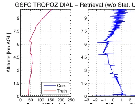
GSFC TROPOZ DIAL − Retrieval (w/o Stat. Unc.)
Figure 6. The left panel shows the retrieved ozone mixing ratios from the TROPOZopt ozone profiles as compared to the known ozone profile used in the simulated lidar return signal without the addition of statistical noise. The right panel shows the percent dif-ference from the known profile and retrieved profile.
acquisition system, which is 250 MHz or 4.0 ns. This correc-tion can be applied as
Ct=
Cm
1−CmTd
, (9)
where the true photon count rate (Ct) can be expressed as a function of the measured count rates (CM) and a dead time (Td) parameter (Lampton and Bixler, 1985).
When this theoretical value was used with the current re-trieval, it did not appear to completely correct for the detector saturation (pulse pile-up). Upon looking at this closer, a bin registration issue was found in the algorithm and was subse-quently adjusted to correctly implement Eq. (9).
The left panel of Fig. 5 shows the corrected, uncorrected and truth profiles for the known ozone profile. The right panel shows the percent difference between each of these profiles. The saturation correction is particularly important in the lower regions of each channel, and an improper al-gorithm may lead to biases upwards of 20 %. Based on the percent difference plot in the right side of Fig. 5, the differ-ence in this correction is<1 % and this will be implemented in the TROPOZoptozone retrieval.
3.5 TROPOZoptretrieval algorithm before the addition of statistical noise
retrieval and known profile without the addition of statisti-cal noise. The spikes in the right panel correspond to abrupt ozone gradients in the simulated ozone profile and are not expected to occur as sharply in the natural atmosphere.
Although it would be physically impossible to deter-mine this percent difference in the real atmosphere with an ozonesonde, this exercise allows the TROPOZoptretrieval to biases to be completely quantified before real atmospheric noise is involved. The percent differences have been quanti-fied to be mostly within ±1 % of the known ozone profile. With the addition of statistical noise, these biases can grow much larger and an optimization scheme is shown in the fol-lowing section.
4 TROPOZoptvariable vertical-resolution scheme and uncertainty analysis
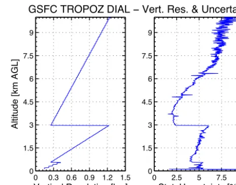
As mentioned before, the TROPOZ retrieval algorithm orig-inally implemented a constant vertical resolution of 375 m below 2.75 km and 750 m above 2.75 km. The left panel of Fig. 7 depicts the new TROPOZopt retrieval effective vertical-resolution scheme. These values are coupled directly to the FWHM of the steady-state SG filter coefficients asso-ciated with the window size as described in the “Numerical derivative” section of this paper.
Because a bias naturally occurs due to the decrease in the SNR with altitude, it is favorable to increase the number of points of the derivative low-pass filter used for data process-ing (Godin et al., 1999). This is evident in the large differ-ence near the 3 km join region, in which the lower channel’s SNR is decreasing and more data points are needed to pro-vide an accurate ozone profile. However, the adjoining upper channel has a sufficiently high SNR to properly perform the retrieval. The large gradient in the SNR, and therefore the vertical resolution, can mostly be attributed to physical hard-ware parameters in the TROPOZ system such as transmitted laser pulse power, telescope diameter, FOV, and various op-tical filters. Although Fig. 7 presents an optimized verop-tical- vertical-resolution scheme for the hardware of the lidar system, it also allows higher-resolution data throughout the dynamic PBL in order to characterize ozone features.
The TROPOZ detects individual photons through the use of photon counting and PMTs. The signal collected by these PMTs follows Poisson statistics (Megie et al., 1985; Pa-payannis et al., 1990), and the statistical uncertainty of the ozone concentrations is shown in the right panel of Fig. 7. The statistical uncertainty at a given range can be calculated as
NO3(i, z)= 1 2NO31σO31ze
s
S(i, z)+Pb(i, z)+Pd(i, z)
S(i, z)2 , (10)
whereS,Pb, andPdare the atmospheric backscattered sig-nal, background radiation, and dark counts of the detector
0 2.5 5 7.5 10
0 1.5 3 4.5 6 7.5 9
Stat. Uncertainty [%] 0 0.3 0.6 0.9 1.2 1.5
0 1.5 3 4.5 6 7.5 9
Vertical Resolution [km]
Altitude [km AGL]
GSFC TROPOZ DIAL − Vert. Res. & Uncertainty
Figure 7. The left panel shows the associated vertical resolution in the TROPOZoptretrieval algorithm, which is derived from the win-dow size of the SG differentiation filter. The right panel shows the statistical uncertainty in the system associated with these vertical resolutions, which is an approximation for the overall uncertainty for the TROPOZopt.
at the DIAL wavelengthi. The total statistical uncertainty is then calculated from the statistical uncertainty from each DIAL wavelength added in quadrature. The effective vertical resolution, which is based on the SG filter window size, is denoted as1ze and the differential ozone absorption cross
section is denoted as1σO3.
The statistical uncertainty is related to the square root of the total PMT counts, both those that are relevant to the re-trieval of ozone number density and those that are counts due to systematic uncertainties. Although this analysis was per-formed with a 10 min average of simulated data, by integrat-ing profiles for a longer duration, the backscattered signal termSbecomes much larger than thePbandPdterms. For this reason, the temporal resolution is inherently built into the statistical uncertainty of the system and averaging many data sets is beneficial to the resultant uncertainty in the system.
0 50 100 150 200 250 0
1.5 3 4.5 6 7.5 9
Ozone MR [ppbv]
Altitude [km AGL]
TROPOZ opt TROPOZ Truth
−045 −30 −15 0 15 30 45
1.5 3 4.5 6 7.5 9
Ozone Difference [%]
−030 −20 −10 0 10 20 30
1.5 3 4.5 6 7.5 9
Overall Improvement [%]
GSFC TROPOZ DIAL − Final Retrieval
0 50 100 150 200 250 0
1.5 3 4.5 6 7.5 9
Ozone MR [ppbv]
Altitude [km AGL]
TROPOZOpt. TROPOZ Truth
−450 −30−15 0 15 30 45 1.5
3 4.5 6 7.5 9
Ozone Difference [%]
−300 −20−10 0 10 20 30 1.5
3 4.5 6 7.5 9
Overall Improvement [%]
3.5% GSFC TROPOZ DIAL − Final Retrieval
Figure 8. The left panel compares the final retrieved ozone concentration from the previous TROPOZ retrieval and the optimized retrieval (TROPOZopt) to the known ozone profile used in the simulated lidar return signal. The center panel shows the differences in percentage from the known profile and retrieved TROPOZ and TROPOZoptprofiles. The right panel shows the improvement from the optimized TROPOZopt retrieval and the original TROPOZ retrieval in percentage. The mean improvement (red line) is 3.5 %.
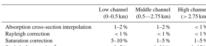
Table 1. Summary of the improvements associated with the optimized GSFC TROPOZ DIAL algorithm as compared to the initial algorithm in Sullivan et al. (2014).
Low channel Middle channel High channel (0–0.5 km) (0.5—2.75 km) (>2.75 km)
Absorption cross-section interpolation 1–2 % 1–2 % <1 %
Rayleigh correction <1 % <1 % <1 %
Saturation correction 5–10 % 1–5 % 1–5 %
Statistical uncertaintya 1–5 % 1–11 % 1–15 %
aImprovements due to optimization of the vertical resolution (Fig. 7).
5 Comparison of the original TROPOZ and TROPOZoptretrieval algorithms
The left panel of Fig. 8 shows the original TROPOZ retrieval (Fig. 1), the optimized TROPOZ retrieval (TROPOZopt) and the truth ozone profile. The TROPOZoptretrieval has imple-mented all of the changes and corrections described through-out the previous sections of this paper including the opti-mized vertical-resolution scheme from Fig. 7.
The middle panel of Fig. 8 shows the percent difference between each of the retrievals and the truth profile. Due to the optimized vertical smoothing scheme, the TROPOZopt algo-rithm is able to produce ozone profiles nearly 200 m lower (from 675 to 500 m) than the previous TROPOZ retrieval. The bin registration error that was identified with the satu-ration correction is also adjusted in the final TROPOZopt re-trieval. This adjustment shows a direct reduction in percent difference near the retrieval join regions of nearly 5 % from 675 to 800 m and 10 % from 2.75 to 3 km. This panel also shows reductions mostly between 5 and 15 % in the percent difference of the upper tropospheric retrieval as compared to the previous algorithm.
The right panel in Fig. 8 serves as a visual summary to quantify the improvement gained from this optimization pro-cess. The improvement was calculated from the difference in the absolute value of each difference profile in the middle panel Fig. 8 and can be written as
Improvement%= |TROPOZ%| − |TROPOZopt%|. (11) The overall profile mean improvement from the original re-trieval to the TROPOZopt retrieval (red line) is 3.5 %. In terms of ozone concentrations, this mean improvement is somewhere between 2 and 4 ppbv. The largest improvements occur in the upper atmosphere where the retrieval perfor-mance and vertical resolution were optimized. Specifically, some of the retrieved ozone concentrations above 4.5 km have improved greatly by more than 10 %.
cor-0 50 100 150 200 250 0 1.5 3 4.5 6 7.5 9
Ozone MR [ppbv]
Altitude [km AGL]
19−Sep−2013 19:03 UTC
TROPOZopt
ECC
0 50 100 150 200 250 0 1.5 3 4.5 6 7.5 9
Ozone MR [ppbv]
25−Oct−2013 17:44 UTC
0 50 100 150 200 250 0 1.5 3 4.5 6 7.5 9
Ozone MR [ppbv]
18−Dec−2013 17:24 UTC
0 50 100 150 200 250 0 1.5 3 4.5 6 7.5 9
Ozone MR [ppbv]
17−Apr−2014 06:59 UTC
−40−30−20−10 0 10 20 30 40 0 1.5 3 4.5 6 7.5 9
Ozone Difference [%]
Mean Difference (±2 )
0 50 100 150 200 250 0 1.5 3 4.5 6 7.5 9
Ozone MR [ppbv]
Altitude [km AGL]
19−Sep−2013 19:03 UTC
TROPOZopt
ECC
0 50 100 150 200 250 0 1.5 3 4.5 6 7.5 9
Ozone MR [ppbv] 25−Oct−2013 17:44 UTC
0 50 100 150 200 250 0 1.5 3 4.5 6 7.5 9
Ozone MR [ppbv] 18−Dec−2013 17:24 UTC
0 50 100 150 200 250 0 1.5 3 4.5 6 7.5 9
Ozone MR [ppbv] 17−Apr−2014 06:59 UTC
−40−30−20−10 0 10 20 30 40 0 1.5 3 4.5 6 7.5 9
Ozone Difference [%] Mean Difference (±2 )
0 50 100 150 200 250
0 1.5 3 4.5 6 7.5 9
Ozone MR [ppbv]
Altitude [km AGL]
19−Sep−2013 19:03 UTC
TROPOZopt
ECC
0 50 100 150 200 250
0 1.5 3 4.5 6 7.5 9
Ozone MR [ppbv] 25−Oct−2013 17:44 UTC
0 50 100 150 200 250
0 1.5 3 4.5 6 7.5 9
Ozone MR [ppbv] 18−Dec−2013 17:24 UTC
0 50 100 150 200 250
0 1.5 3 4.5 6 7.5 9
Ozone MR [ppbv] 17−Apr−2014 06:59 UTC
−080−60−40−20 0 20 40 60 80 1.5 3 4.5 6 7.5 9
Ozone Difference [%] Mean Difference (±2 )
0 50 100 150 200 250 0 1.5 3 4.5 6 7.5 9
Ozone MR [ppbv]
Altitude [km AGL]
19−Sep−2013 19:03 UTC
TROPOZ
opt
ECC
0 50 100 150 200 250 0 1.5 3 4.5 6 7.5 9
Ozone MR [ppbv] 25−Oct−2013 17:44 UTC
0 50 100 150 200 250 0 1.5 3 4.5 6 7.5 9
Ozone MR [ppbv] 18−Dec−2013 17:24 UTC
0 50 100 150 200 250 0 1.5 3 4.5 6 7.5 9
Ozone MR [ppbv] 17−Apr−2014 06:59 UTC
−40−30−20−10 0 10 20 30 40 0 1.5 3 4.5 6 7.5 9
Ozone Difference [%] Mean Difference (±2 )
0 50 100 150 200 250 0 1.5 3 4.5 6 7.5 9
Ozone MR [ppbv]
Altitude [km AGL]
19−Sep−2013 19:03 UTC
TROPOZopt ECC
0 50 100 150 200 250 0 1.5 3 4.5 6 7.5 9
Ozone MR [ppbv]
25−Oct−2013 17:44 UTC
0 50 100 150 200 250 0 1.5 3 4.5 6 7.5 9
Ozone MR [ppbv]
18−Dec−2013 17:24 UTC
0 50 100 150 200 250 0 1.5 3 4.5 6 7.5 9
Ozone MR [ppbv]
17−Apr−2014 06:59 UTC
−50−40−30−20−10 0 10 20 30 40 500 1.5 3 4.5 6 7.5 9
Relative Difference [%]
Mean Ozone Difference
0 50 100 150 200 250 0 1.5 3 4.5 6 7.5 9
Ozone MR [ppbv]
Altitude [km AGL]
19−Sep−2013 19:03 UTC
TROPOZopt ECC
0 50 100 150 200 250 0 1.5 3 4.5 6 7.5 9
Ozone MR [ppbv]
25−Oct−2013 17:44 UTC
0 50 100 150 200 250 0 1.5 3 4.5 6 7.5 9
Ozone MR [ppbv]
18−Dec−2013 17:24 UTC
0 50 100 150 200 250 0 1.5 3 4.5 6 7.5 9
Ozone MR [ppbv]
17−Apr−2014 06:59 UTC
−050−40−30−20−10 0 10 20 30 40 50 1.5 3 4.5 6 7.5 9
Relative Difference [%]
Mean Ozone Difference
Diff ±2
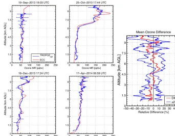
Figure 9. Comparisons between four nearby ECC ozonesonde launches and the updated TROPOZoptretrieval algorithm.
rection discovered during this process. The improvement is largest, 5–10 %, in the low channel because the signals are nearest to saturation, but still had a non-negligible effect, 1– 5 %, in the middle and high channels. As discussed previ-ously, large improvements, upwards of 10–15 %, in the mid-dle and high channels corresponded directly to the optimized vertical-resolution scheme.
6 Final TROPOZoptretrieval as compared to ozonesondes
After implementing the TROPOZopt retrieval algorithm it was important to analyze real lidar signals profiles that are convolved with sources of noise. This allows for confirma-tion that the real ambient sky radiaconfirma-tion is being correctly accounted for in the final ozone mixing ratio profile. The aerosol correction from Sullivan et al. (2014) has also been applied to the real lidar signals. Although the theoretical dead time correction value is 4.00 ns, based on the counting rate of the transient recorder, this is rarely physically achieved. For this reason, larger values between 4 and 5 ns are used and were empirically determined by comparing the lidar return signal to a model atmosphere or from ozonesonde data.
Figure 9 shows four different ozonesonde launches as compared to the new TROPOZoptalgorithm, and the uncer-tainty bars represent the statistical unceruncer-tainty of the mea-surement described in Fig. 7. These lidar profiles are 10 min averages and are each centered around 19 September 2013
at 19:03 UTC, 25 October 2013 at 17:44 UTC, 18 Decem-ber 2013 at 17:24 UTC, or 17 April 2014 at 06:59 UTC. The ozonesondes were launched by the Howard Univer-sity Beltsville Center for Climate Systems Observation. The launch site (39.05◦N, 76.88◦W) is approximately 8 km from the lidar site which is close enough to assume similar but not identical tropospheric micrometeorology in the dynamic daytime PBL. These comparison times were chosen to max-imize overlap of the two instruments based on the sonde’s proximity to the lidar and ascent rate.
with the ozonesonde profile for the lower altitude ranges, but it begins to differ in the upper altitudes. The final ozonesonde comparison on 17 April 2014 at 06:59 UTC shows excel-lent agreement between the ozonesonde and the TROPOZopt -retrieved ozone mixing ratio. This a nighttime ozonesonde launch, in which the sky background radiation is negligible and the SNR is naturally higher. These combine with a very low concentration of ozone to yield a fairly low statistical uncertainty in the measurement.
7 Conclusions
This paper serves as the first paper to concentrate on the op-timization of the GSFC TROPOZ DIAL retrieval. This pa-per is focused on ensuring that the TROPOZ algorithm is accurately quantifying ozone concentrations, and the follow-ing paper will focus on a robust uncertainty analysis. Usfollow-ing simulated lidar returns has shown to be beneficial for testing a new operational version of TROPOZ analysis algorithm. The advantage of using simulated signals is that it is possi-ble to turn varying effects on and off in order to investigate differences between the retrieval and the known truth profile. These differences could never have been truly investigated with actual lidar returns and instantaneous ozonesonde pro-files because the state of the atmosphere is never precisely known.
One key improvement from this analysis came from opti-mizing the vertical-resolution scheme from a previously con-stant resolution. These improvements were upwards of 10 % above 4.5 km. The overall improvement was 3.5 % from the previous retrieval, and it was able to extend the lower limit of the range of ozone retrievals by nearly 200 m. The au-thors believe that this analysis has significantly added to the confidence that the TROPOZ retrieval algorithm is properly quantifying ozone concentrations. Application of this tech-nique will be recommended to all other TOLNet lidars for validation, optimization, and consistency purposes.
Acknowledgements. This work was supported by UMBC/JCET
(Task #374, Project 8306), the Maryland Department of the Environment (MDE, Contract #U00P4400079), NOAA-CREST CCNY Foundation (Sub-Contract #49173B-02) and the National Aeronautics and Space Administration. Work at the Jet Propulsion Laboratory, California Institute of Technology, was carried out under contract with the National Aeronautics and Space Admin-istration. The authors gratefully acknowledge support provided by NASA HQ, the NASA Tropospheric Chemistry Program and the Tropospheric Ozone Lidar Network (TOLNet). Thanks to Raymond M. Hoff for additional support and knowledge of lidar techniques. Also, thanks to the Howard University – Beltsville Cen-ter for Climate Systems Observation for launching the ozonesondes necessary to continue validating this system.
Edited by: G. Pappalardo
References
Alvarez, R. J., Senff, C. J., Langford, A. O., Weickmann, A. M., Law, D. C., Machol, J. L., Merritt, D. A., Marchbanks, R. D., Sandberg, S. P., Brewer, W. A., Hardesty, R. M., and Banta, R. M.: Development and application of a compact, tunable, solid-state airborne ozone lidar system for boundary layer profiling, J. Atmos. Ocean.Technol., 28, 1258–1272, 2011.
Boor, C. D.: A practical guide to splines, Mathematics of Computa-tion, 1978.
Eberhard, W. L.: Correct equations and common approximations for calculating Rayleigh scatter in pure gases and mixtures and evaluation of differences, Appl. Opt., 49, 1116–1130, 2010. Godin, S., Carswell, A. I., Donovan, D. P., Claude, H., Steinbrecht,
W., McDermid, I. S., McGee, T. J., Gross, M. R., Nakane, H., Swart, D. P. J., Bergwerff, H. B., Uchino, O., von der Gathen, P., and Neuber, R.: Ozone differential absorption lidar algorithm intercomparison, Appl. Opt., 38, 6225–6236, 1999.
Hedin, A. E.: Extension of the MSIS thermosphere model into the middle and lower atmosphere, J. Geophys. Res.-Space, 96, 1159–1172, 1991.
Keckhut, P., McDermid, S., Swart, D., McGee, T., Godin-Beekmann, S., Adriani, A., Barnes, J., Baray, J.-L., Bencherif, H., Claude, H., di Sarra, A. G., Fiocco, G., Hansen, G., Hauchecorne, A., Leblanc, T., Lee, C. H., Pal, S., Megie, G., Nakane, H., Neuber, R., Steinbrecht, W., and Thayer, J.: Review of ozone and temperature lidar validations performed within the framework of the Network for the Detection of Stratospheric Change, J. Environ. Monit., 6, 721–733, doi:10.1039/B404256E, 2004a.
Keckhut, P., McDermid, S., Swart, D., McGee, T., Godin-Beekmann, S., Adriani, A., Barnes, J., Baray, J.-L., Bencherif, H., Claude, H., di Sarra, A. G., Fiocco, G., Hansen, G., Hauchecorne, A., Leblanc, T., Lee, C. H., Pal, S., Megie, G., Nakane, H., Neuber, R., Steinbrecht, W., and Thayer, J.: Review of ozone and temperature lidar validations performed within the framework of the Network for the Detection of Stratospheric Change, J. Environ. Monit., 6, 721–733, doi:10.1039/B404256E, 2004b.
Lampton, M. and Bixler, J.: Counting efficiency of systems hav-ing both paralyzable and nonparalyzable elements, Rev. Sci. In-strum., 56, 164–165, 1985.
Leblanc, T., McDermid, I. S., Hauchecorne, A., and Keckhut, P.: Evaluation of optimization of lidar temperature analysis al-gorithms using simulated data, J. Geophys. Res.-Atmos., 103, 6177–6187, doi:10.1029/97JD03494, 1998.
Malicet, J., Daumont, D., Charbonnier, J., Parisse, C., Chakir, A., and Brion, J.: Ozone UV spectroscopy. II. Absorption cross-sections and temperature dependence, J. Atmos. Chem., 21, 263– 273, doi:10.1007/BF00696758, 1995.
Megie, G. J., Ancellet, G., and Pelon, J.: Lidar measurements of ozone vertical profiles, Appl. Opt., 24, 3454–3463, 1985. Papayannis, A., Ancellet, G., Pelon, J., and Mégie, G.:
Multiwave-length lidar for ozone measurements in the troposphere and the lower stratosphere, Appl. Opt., 29, 467–476, 1990.
Savitzky, A. and Golay, M. J. E.: Smoothing and differentiation of data by simplified least squares procedures, Anal. Chem., 36, 1627–1639, 1964.
Sullivan, J. T., McGee, T. J., Sumnicht, G. K., Twigg, L. W., and Hoff, R. M.: A mobile differential absorption lidar to mea-sure sub-hourly fluctuation of tropospheric ozone profiles in the Baltimore-Washington, D.C. region, Atmos. Meas. Tech., 7, 3529–3548, doi:10.5194/amt-7-3529-2014, 2014.
Sullivan, J. T., McGee, T. J., De Young, R., Sumnicht, G. K., Twigg, L. W., Pliutau, D., Carrion, W., and Knepp, T.: Results from the NASA GSFC and LaRC ozone lidar intercomparison: New mo-bile tools for atmospheric research, J. Atmos. Ocean. Technol., 32, 1779–1795, 2015.
Thompson, A. M., Witte, J. C., McPeters, R. D., Oltmans, S. J., Schmidlin, F. J., Logan, J. A., Fujiwara, M., Kirch-hoff, V. W. J. H., Posny, F., Coetzee, G. J. R., Hoegger, B., Kawakami, S., Ogawa, T., Johnson, B. J., Vömel, H., and Labow, G.: Southern Hemisphere Additional Ozoneson-des (SHADOZ) 1998–2000 tropical ozone climatology 1. Com-parison with Total Ozone Mapping Spectrometer (TOMS) and ground-based measurements, J. Geophys. Res.-Atmos., 108, D2, doi:10.1029/2001JD000967, 2003.
Thuburn, J.: UGAMP Internal Report, Tech. Rep. 16, University of Exeter, UK, 1992.
US Standard: US standard atmosphere, 1976, Adopted by the United States Committee on Extension to the Standard Atmo-sphere, National Oceanic and Amospheric Administration, US Govt. Print. Off., Washington, 1976.