www.the-cryosphere.net/10/1721/2016/ doi:10.5194/tc-10-1721-2016
© Author(s) 2016. CC Attribution 3.0 License.
Evaluation of air–soil temperature relationships simulated by land
surface models during winter across the permafrost region
Wenli Wang1, Annette Rinke1,2, John C. Moore1, Duoying Ji1, Xuefeng Cui3, Shushi Peng4,17,18, David M. Lawrence5, A. David McGuire6, Eleanor J. Burke7, Xiaodong Chen21, Bertrand Decharme9, Charles Koven10,
Andrew MacDougall11, Kazuyuki Saito12,15, Wenxin Zhang13,19, Ramdane Alkama9,16, Theodore J. Bohn8, Philippe Ciais18, Christine Delire9, Isabelle Gouttevin4, Tomohiro Hajima12, Gerhard Krinner4,17,
Dennis P. Lettenmaier8, Paul A. Miller13, Benjamin Smith13, Tetsuo Sueyoshi14, and Artem B. Sherstiukov20 1College of Global Change and Earth System Science, Beijing Normal University, Beijing, China
2Alfred Wegener Institute Helmholtz Centre for Polar and Marine Research (AWI), Potsdam, Germany 3School of System Science, Beijing Normal University, Beijing, China
4The Laboratory of Glaciology, French National Center for Scientific Research, Grenoble, France 5National Center for Atmospheric Research, Boulder, USA
6US Geological Survey, Alaska Cooperative Fish and Wildlife Research Unit, University of Alaska Fairbanks, Fairbanks, AK, USA
7Met Office Hadley Centre, Exeter, UK
8School of Earth and Space Exploration, Arizona State University, Tempe, AZ, USA
9Groupe d’étude de l’Atmosphère Météorologique, Unité mixte de recherche CNRS/Meteo-France, Toulouse cedex, France 10Lawrence Berkeley National Laboratory, Berkeley, CA, USA
11School of Earth and Ocean Sciences, University of Victoria, Victoria, BC, Canada 12Japan Agency for Marine-Earth Science and Technology, Yokohama, Japan
13Department of Physical Geography and Ecosystem Science, Lund University, Lund, Sweden 14National Institute of Polar Research, Tachikawa, Japan
15University of Alaska Fairbanks, Fairbanks, AK, USA
16L’Institute for Environment and Sustainability (IES), Ispra, Italy 17Université Grenoble Alpes, LGGE, Grenoble, France
18Climate and Environment Sciences Laboratory, the French Alternative Energies and Atomic Energy Commission, French National Center for Scientific Research, University of Versailles Saint-Quentin-en-Yvelines, Saclay, France
19Center for Permafrost (CENPERM), Department of Geosciences and Natural Resource Management, University of Copenhagen, Copenhagen, Denmark
20All-Russian Research Institute of Hydrometeorological Information – World Data Centre, Obninsk, Russia 21Department of Civil and Environmental Engineering, University of Washington, Seattle, WA, USA
Correspondence to:Duoying Ji ([email protected])
Abstract.A realistic simulation of snow cover and its ther-mal properties are important for accurate modelling of per-mafrost. We analyse simulated relationships between air and near-surface (20 cm) soil temperatures in the Northern Hemi-sphere permafrost region during winter, with a particular fo-cus on snow insulation effects in nine land surface models, and compare them with observations from 268 Russian sta-tions. There are large cross-model differences in the simu-lated differences between near-surface soil and air tempera-tures (1T; 3 to 14◦C), in the sensitivity of soil-to-air tem-perature (0.13 to 0.96◦C◦C−1), and in the relationship be-tween 1T and snow depth. The observed relationship be-tween1T and snow depth can be used as a metric to evalu-ate the effects of each model’s representation of snow insu-lation, hence guide improvements to the model’s conceptual structure and process parameterisations. Models with better performance apply multilayer snow schemes and consider complex snow processes. Some models show poor perfor-mance in representing snow insulation due to underestima-tion of snow depth and/or overestimaunderestima-tion of snow conduc-tivity. Generally, models identified as most acceptable with respect to snow insulation simulate reasonable areas of near-surface permafrost (13.19 to 15.77 million km2). However, there is not a simple relationship between the sophistication of the snow insulation in the acceptable models and the sim-ulated area of Northern Hemisphere near-surface permafrost, because several other factors, such as soil depth used in the models, the treatment of soil organic matter content, hy-drology and vegetation cover, also affect the simulated per-mafrost distribution.
1 Introduction
Present-day permafrost simulations by global climate mod-els are limited and future projections contain high, model-induced uncertainty (e.g. Slater and Lawrence, 2013; Koven et al., 2013). Most of the model biases and cross-model dif-ferences in simulating permafrost area are due to inaccurate atmospheric simulation, e.g. of air temperature and precipi-tation, deficient simulation of snow and soil temperature and the coupling between atmosphere and land surface. In winter, the snow insulation effect is a key process for air–soil tem-perature coupling. Its strength depends on the snow depth, areal coverage, snow density and conductivity (see overview by Zhang, 2005). Many individual model studies have shown the strong impact of snow parameterisations on soil temper-ature simulations (e.g. Langer et al., 2013; Dutra et al., 2012; Gouttevin et al., 2012; Essery et al., 2013; Wang et al., 2013; Jafarov et al., 2014). Most importantly, these studies showed that the consideration of wet snow metamorphism and snow compaction, improved snow thermal conductivity and multi-layer snow schemes can improve the simulation of snow dy-namics and soil temperature. Parameterisations that take into
account snow compaction (e.g. related to overburden pres-sure, thermal metamorphism and liquid water) work better than simpler schemes such as an exponential increase of den-sity with time (Dutra et al., 2010). The influence of snow thermal conductivity on soil temperature has been demon-strated by many model studies (e.g. Bartlett et al., 2006; Saha et al., 2006; Vavrus, 2007; Nicolsky et al., 2007; Dankers et al., 2011; Gouttevin et al., 2012). Winter soil temperature can change by up to 20 K simply by varying the snow thermal conductivity by 0.1–0.5 W m−1K−1(Cook et al., 2008). The snow insulation effect also plays an important role for the Arctic soil temperature response to climate change and there-fore for future near-surface permafrost thawing and soil car-bon vulnerability (e.g. Schuur et al., 2008). Shallower snow can reduce soil warming while shorter snow season can en-hance soil warming (Lawrence and Slater, 2010). The model skill in atmosphere–soil coupling with the concomitant snow cover in the Arctic is an important factor in the assessment of limitations and uncertainty of carbon mobility estimates (Schaefer et al., 2011).
The Snow Models intercomparison project (SnowMIP; Essery et al., 2009) and the Project for Intercomparison of Land Surface Parameterization Schemes (PILPS) Phase 2e (Slater et al., 2001) examined the snow simulations of an ensemble of land surface schemes for the midlatitudes. However, until now there has been no attempt to evaluate the air–soil temperature relationship in the Northern Hemi-sphere permafrost region and the detailed role of snow depth therein across an ensemble of models. In such an investi-gation, a first suitable approach is the evaluation of stand-alone (offline) land surface models (LSMs). The retrospec-tive (1960–2009) simulations from the model integration group of the Permafrost Carbon Network (PCN; http://www. permafrostcarbon.org) provide an opportunity to evaluate an ensemble of nine state-of-the-art LSMs. Here, the LSMs are run with observation-based atmospheric forcing, meaning that snow depth is not influenced by biases in the atmospheric forcing in a coupled model set-up. The evaluation of the of-fline modelled air temperature–snow depth–near-surface soil temperature relationship in winter is therefore important for revealing a model’s skill in representing the effects of snow insulation.
Most of the LSMs participating in PCN are the land sur-face modules of Earth system models (ESMs) participat-ing in the Coupled Model Intercomparison Project (CMIP5; http://cmip-pcmdi.llnl.gov/cmip5/) although in some cases different versions were used for PCN and CMIP5 simula-tions. Thus, the results we present can guide the correspond-ing evaluation of these ESMs, though analysis of coupled model results requires consideration of couplings between model components and is necessarily more complex.
winter, with a particular focus on the snow insulation effect. For the latter we analyse the impact of snow depth on the dif-ference between near-surface soil and air temperatures. Our related key questions are the following: how well do the mod-els represent the observed spatial pattern of the air–soil tem-perature difference in winter and how it is controlled by snow depth? What is the range of the simulated air–soil tempera-ture relationship across the model ensemble? To the greatest extent possible, we try to relate the performance of the mod-els to their snow schemes. With this aim in mind, a simulta-neous analysis of simulated air and near-surface soil temper-atures and snow depth is presented and compared with those from a novel data set of Russian station observations. We used this data set because it has been compiled within PCN, and it is hard to find other station data sets which provide si-multaneous observations of both air and soil temperatures as well as snow depth over a long period.
In Sect. 2, we describe the model simulations, the station observations used for evaluation and the analysis methods. In Sect. 3, we present a detailed analysis of near-surface air temperature–snow depth–soil temperature relationships in winter. In Sect. 4, we discuss the roles of atmospheric forc-ing and model processes. In Sect. 5, we investigate the rela-tionship between simulated snow insulation and permafrost area. We summarise our findings and present conclusions in Sect. 6.
2 Data and analysis 2.1 Models
We use data from nine LSMs participating in the PCN, including CLM4.5, CoLM, ISBA, JULES, LPJ-GUESS, MIROC-ESM, ORCHIDEE, UVic and UW-VIC. For de-tailed information about the models and simulations we refer to Rawlins et al. (2015), Peng et al. (2015) and McGuire et al. (2016). The total soil depth for soil thermal calculations ranges from 3 m (divided into 8 layers) in LPJ-GUESS to 250 m (divided into 14 layers) in UVic. The physical proper-ties of the soil differ among the models as well, and four of them (CLM4.5, ISBA, UVic, UW-VIC) include organic hori-zons. Three models (ISBA, LPJ-GUESS, UW-VIC) do not archive soil subgrid results and provide only area-weighted ground temperature (i.e. averaged over wetlands and vege-tated areas, and in some cases lake fractions).
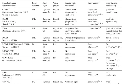
Table 1 lists relevant snow model details. One model (UVic) uses an implicit snow scheme which replaces the upper soil column with snow-like properties, i.e. the near-surface soil layer takes the temperature of the air–snow in-terface. The other models use separate snow layers on top of the ground, either a single bucket (LPJ-GUESS, UW-VIC) or multilayer snow schemes (CLM4.5, CoLM, ISBA, JULES, MIROC-ESM, ORCHIDEE). Snow insulation is ex-plicitly considered in all models: increasing snow depth
in-creases the insulation effect. Most models consider the ef-fect of varying snow density on insulation (Table 1). This is parameterised by a snow conductivity–density relation-ship. Some of the models (LPJ-GUESS, MIROC-ESM, OR-CHIDEE, UVic) use a fixed snow density, consider only dry snow and no compaction effects, while others represent liq-uid water in snow and different processes for snow densifi-cation such as mechanical compaction and thermal and de-structive metamorphism (Table 1).
The simulations were generally run for the period 1960– 2009, although some simulations were stopped a few years earlier. Each model team was free to choose appropriate driv-ing data sets for weather and climate, atmospheric CO2, ni-trogen deposition, disturbance, land cover, soil texture, etc. However, the climate forcing data (surface pressure, surface incident longwave and shortwave radiation, near-surface air temperature, wind and specific humidity, rain and snowfall rates) are from gridded observational data sets (e.g. CRUN-CEP, WATC; Table S1 in the Supplement). The exception is MIROC-ESM, which was run as a fully coupled model, forced by its own simulated climate. Mean annual air tem-perature simulated by MIROC-ESM for the permafrost re-gion was within the range (−7.2 to 2.2◦C) of the other forc-ing data sets used in this study and the trend in near-surface air temperature (+0.03◦C yr−1)was the same for all forc-ing data sets. However, MIROC-ESM had both the highest annual precipitation (range 433 to 686 mm) and the highest trend in annual precipitation (range−2.1 to+0.8 mm yr−1)
among the forcing data sets.
The spatial domain of interest is the Northern Hemi-sphere permafrost land regions. Our analysis is based on the 0.5◦×0.5◦-resolution gridded driving and modelled data for winter (DJF) 1980–2000.
2.2 Observations
Table 1.PCN snow model details.
Model reference Snow Snow Water Liquid water Snow density3 Snow thermal for snow scheme scheme1 layers phases treatment2 conductivity4
CLM4.5 ML Dynamic Liquid, Bucket-type depends on quadratic Swenson and Lawrence (2012) (max. 5) ice prognostic in snow depth; equation onρ Oleson et al. (2013) each layer compaction3a, b, c
CoLM ML Dynamic Liquid, Bucket-type depends on quadratic Dai et al. (2003) (max. 5) ice prognostic in snow depth; equation onρ Ji et al. (2014) each layer compaction3a, b, c
ISBA ML Static Liquid, ice, Diagnosed from compaction3a, b quadratic equation on Boone and Etchevers (2001) (3) vapour snow temperature, ρ, contribution due
mass, density to vapour transfer
JULES ML Dynamic Liquid, ice, Bucket-type prognostic compaction3a power equation Best et al. (2011) (max. 3) vapour in each layer onρ
LPJ-GUESS Wania et al. (2009) BL Static Ice Not fixed fixed
Gerten et al. (2004) (1) represented 362 kg m−3 0.196 W m−1K−1
MIROC-ESM ML Dynamic Ice Not fixed fixed
Takata et al. (2003) (max. 3) represented 300 kg m−3 0.3 W m−1K−1
ORCHIDEE ML Dynamic Ice Not fixed fixed
Gouttevin et al. (2012) (max. 7) represented 330 kg m−3 0.25 W m−1K−1 for tundra, 0.042 W m−1K−1 for taiga
UVic I Static Ice Not fixed bulk
Meissner et al. (2003) (1) represented 330 kg m−3 conductivity Avis (2012)
UW-VIC BL Dynamic Liquid, ice, Constant liquid compaction3a, b fixed
Andreadis et al. (2009) (max. 2) vapour water holding capacity 0.7 Wm−1K−1 1ML: Multilayer, BL: Bulk-layer, I: Implicit; according to Slater et al. (2001).2Not represented means dry snow.3Processes for densification of the snow:(a)mechanical compaction (due to the weight of the overburden),(b)thermal metamorphosis (via the melting–refreezing process),(c)destructive metamorphism (crystal breakdown due to wind, thermodynamic stress); Anderson (1976), Jordan (1991), Kojima (1967).4quadratic equation onρaccording to Jordan (1991), Anderson (1976); contribution due to vapour transfer according to Sun et al. (1999).
observations could be disturbed by grass cutting during the warm season and the removal of organic materials, mainly at agricultural sites, which may affect the trend in the warm season (Park et al., 2014), but this does not affect our results on the air–upper soil temperature relationship in winter.
Precipitation station data have been compiled from the GSOD data set produced by the National Climatic Data Cen-ter (NCDC; http://www.ncdc.noaa.gov) for all of the stations that are included in the RIHMI-WDC data set. In addition to the station’s ground snow depth observations we use grid-ded snow water equivalent (SWE) data from the GlobSnow-2 product (http://www.globsnow.info/swe/), which have been produced using a combination of passive microwave ra-diometer and ground-based weather station data (Takala et al., 2011). Orographic complexity, vegetation cover and snow state (e.g. wet snow) affect the accuracy of this product. When compared with ground measurements in Eurasia, the GlobSnow product shows root mean square error (RMSE) values of 30 to 40 mm for SWE values below 150 mm, with retrieval uncertainty increases when SWE is above this threshold (e.g. Takala et al., 2011; Muskett, 2012; Klehemet
et al., 2013). In order to be compared with station data, snow depth was then calculated from SWE using a snow density of 250 kg m−3, which is a median observed value in win-ter. Zhong et al. (2014) report snow density values of 180– 250 kg m−3 for tundra/taiga and 156–193 kg m−3for alpine snow classes. Woo et al. (1983) report snow density values of 250–400 kg m−3for various terrain types. Choice of density does not materially affect the results.
All these data have been compiled for winter (DJF) and the same time period of 1980–2000. This period was cho-sen because soil temperature data are sparse before 1980 and the JULES simulation stopped in the year 2000. Compari-son of the simulations with the station data was done using a weighted bilinear interpolation from the four surrounding model grid points onto the station locations.
2.3 Analysis methods
qualita-tively change any of the intervariable relationships found. The focus in our study is on the evaluation of the simulated air–soil temperature relationships, modulated by snow depth. For this, we analyse the winter mean as well as the inter-annual variability (expressed as the standard deviation) of four key variables: near-surface air temperature (Tair), near-surface soil temperature (soil temperature at 20 cm depth;
Tsoil), snow depth (dsnow)and the difference between Tsoil andTair. This difference1T (1T =Tsoil−Tair)is called the air–soil temperature difference. By limiting our analysis to winter only, we are able to attribute the cross-model and model-to-observation differences in 1T primarily to snow insulation effects. In winter, the effects of other factors (e.g. soil moisture, texture) on1T are much smaller than that of snow. Ground surface temperatures were not recorded in the Russian data set, but 20 cm soil depth temperatures were. To test how sensitive results are using 20 cm depth tem-peratures instead of ground surface temtem-peratures, we also analysed model-simulated temperature differences between ground surface andTair, and found no qualitative differences, hence justifying the use of 20 cm observations.
We use the Pearson product–moment correlation coeffi-cient and its significance (von Storch and Zwiers, 1999) to investigate the covariability between1T anddsnow as well as betweenTsoiland its two forcing factors (Tairanddsnow). Before we compute the correlations, we detrended the data by removing a least squares regression line. The calculated correlation maps (i.e. spatial distributions of correlation co-efficients) based on model and observation data, allow com-parison of the spatial patterns of these relationships.
To further examine the functional behaviour between the key variables, we present relation diagrams between pairs of variables (e.g. variation of 1T with change of dsnow). To evaluate the performance of the individual LSMs we cal-culate the RMSE between the observed and modelled re-lationships. We illustrate the dependence of 1T vs. dsnow andTsoil vs.dsnowrelations for threeTair ranges. To distin-guish dry snow pack regimes from those where sporadic melt may occur even in winter, we split Tair into three regimes: the coldest conditions (Tair≤ −25◦C, representing 24 % of observations), the intermediate temperature conditions (−25◦C <Tair≤ −15◦C, representing 42 % of the observa-tions), and the warmest conditions (−15◦C <Tair≤ −5◦C, representing 34 % of observations). Hence it is an indirect separation of temperature-gradient metamorphosis regimes and density-gradient metamorphosis snow pack regimes. Ad-ditionally, we present conditional probability density func-tions (PDFs) of1T for different snow depth and air temper-ature regimes and compare the simulated PDFs with those obtained from station observations.
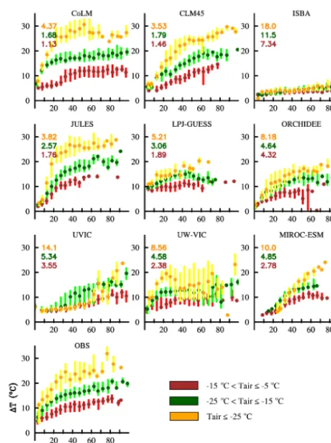
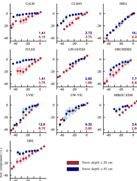
Figure 1.Variation of1T (◦C), the difference between soil tem-perature at 20 cm depth and air temtem-perature with snow depth (cm) for winter 1980–2000. The dots represent the medians of 5 cm snow depth bins and the upper and lower bars indicate the 25th and 75th percentiles, calculated from all Russian station grid points (n=268) and 21 individual winters. The numbers in each model panel indi-cate the RMSE between the observed and modelled relationship. Colours represent different air temperature regimes.
3 Results
3.1 Relationship between air–soil temperature difference and snow depth
The relationship between air–soil temperature difference (1T ) and snow depth (dsnow)in winter (Fig. 1) shows an increase of 1T with increasing dsnow in the Russian sta-tion observasta-tions. The data exhibit a linear relasta-tion between
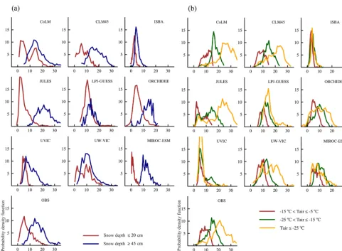
Figure 2.Conditional probability density functions (PDFs) of1T (◦C), the difference between soil temperature at 20 cm depth and air temperature for(a)different snow depth classes and(b)air temperature regimes for winter 1980–2000.
All models reproduce the observed relationship, i.e. in-creasing 1T with increasing dsnow. However, Fig. 1 also shows a wide cross-model spread in the simulated relation-ships and shows that some of the models are not consis-tent with the behaviour in the observations. Only three mod-els (CLM4.5, CoLM, JULES) reproduce the observed 1T
vs.dsnowrelationship reasonably well using a benchmark of RMSE < 5◦C for all temperature regimes. In particular LPJ-GUESS, ORCHIDEE, UVic, UW-VIC, MIROC-ESM show large RMSE for cold air conditions. ISBA stands out overall, with a RMSE of 7–18◦C in all temperature ranges. We con-clude that these models do not adequately represent the fea-tures of the observed1T vs.dsnowrelationship. The scatter in the modelled relationships, indicated by the interquartile range, is of the same order as in the observations, except for ISBA and MIROC-ESM, which produce noticeably smaller variations.
Figure 2a views the1T vs.dsnow relationship in a com-plementary form using the PDFs of 1T for different snow depth regimes. This analysis allows for a detailed evaluation of the snow-regime-dependent 1T separation by
quantify-ing and comparquantify-ing the modal value and width of the different conditional PDFs. Since the Russian snow depths are clearly non-normal in distribution (Fig. S1 in the Supplement, with a median dsnow of 30 cm), we divide the data into “shal-low” (dsnow≤20 cm) and “thick” (dsnow≥45 cm) regimes to separate two snow depth regimes. The modal value of the station-based1T PDF is 5◦C for shallow snow and 14◦C for thick snow; that is, thick snow is a better insulator than thin snow. Based on the 1T PDFs, five models (CoLM, CLM4.5, JULES, ORCHIDEE, MIROC-ESM) successfully separate the1T regimes under different snow depth condi-tions. Their simulated1T PDFs have a smaller modal value for thin snow than for thick snow, like in the observations. The other models clearly fail in separating the1T PDFs for the two different snow depth regimes. However, even for the five successful models, both the shapes and the modal values of the simulated PDFs differ from the observed PDF.
Both Figs. 1 and 2b further indicate that1T is related to
example, the density of fresh fallen snow tends to be much lower under coldTairthan warm (Anderson, 1976), leading to increased insulation (larger1T ). Snow densification is also a function of Tair; for example, depth hoar metamorphosis of the snow pack, which produces more insulation (loosely packed depth-hoar crystals have very low thermal conduc-tivity), is promoted by strong thermal gradients in the snow pack and is typical of continental climates (e.g. Zhang et al., 1996). Therefore, we can expect that the same thickness of snow in colder climates will provide greater insulation than it would in warmer climates.
Our analysis of observations (Figs. 1 and 2b) confirms (i) a larger 1T for colderTair than for warmer Tair (for a given snow depth), (ii) a greater sensitivity of1T to changes in dsnow in colder Tair (Fig. 1) and (iii) a larger modal value of the 1T PDF for colder Tair than for warmer Tair (21◦C forT
air≤ −25◦C and 9◦C for−15◦C <Tair≤ −5◦C; Fig. 2b). These effects are consistent with colder climates having lower density snow packs, and the differences are in line with measurements of snow density variability (Zhong et al., 2014). Additionally, both the interquartile range in Fig. 1 and the width of the PDFs in Fig. 2b become larger asTair cool. This may be related to the formation of depth hoar, which is a very good insulator and its varying presence in the snow pack decouples 1T from dsnow. Cold, thin snow packs tend to contain much more low-density depth hoar than warmer snow packs (e.g. Zhang et al., 1996; Singh et al., 2011). Continental regions have large annual temperature cycles, with greater interannual variability and thinner snow packs than maritime ones. This variability leads to greater scatter and greater sensitivity of the1T vs.dsnow relation-ship in the cold winter regions. An additional cause of scat-ter is that the density of fresh-fallen snow decreases with the decrease of temperature. Accordingly, in the cold Tair regime (Tair≤ −25◦C) we find a larger1T in early winter (November–December), when the snow pack is composed of thinner lower-density fresh snow (and depth hoar), than late winter (January–February; Fig. S2). Under warm conditions (−15◦C <Tair≤ −5◦C) such a separation is not observed.
If we evaluate the models with respect to this observed im-pact ofTairon the1T vs.dsnowrelationship, we demonstrate that some models (CLM4.5, CoLM, JULES) are better able to replicate the effect than others (LPJ-GUESS, MIROC-ESM, ORCHIDEE, UW-VIC; Fig. 1). The latter do not fully replicate the larger1T under coldTairconditions. CLM4.5, CoLM and JULES capture a larger 1T for colder Tair for a givendsnowin agreement with the observations. However, for shallow snow, JULES simulates an increase of1T with increasing dsnow for all temperature ranges that is twice as large as observations. Two models (ISBA, UVic) clearly fail in this evaluation. Poor model performance in reflectingTair influence on the1T vs.dsnowalso manifests itself in regime separation of the PDFs (Fig. 2b). Some models do not sepa-rate the1T regimes under differentTairconditions well or at all (ISBA, LPJ-GUESS, MIROC-ESM, UVic), while others
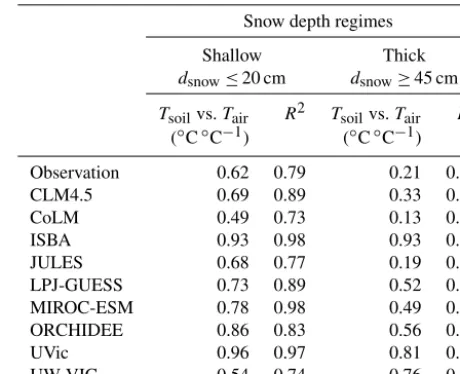
Table 2.Sensitivity of near-surface soil temperature (Tsoil)to air temperature (Tair)in winter (DJF) calculated by the slopes of the linear regression between Tsoil (◦C) and Tair (◦C) for different regimes of snow depth (dsnow), using data from all Russian station grid points and 21 individual winter 1980–2000. All relationships are statistically significant atp≤0.01.
Snow depth regimes
Shallow Thick
dsnow≤20 cm dsnow≥45 cm
Tsoilvs.Tair R2 Tsoilvs.Tair R2
(◦C◦C−1) (◦C◦C−1)
Observation 0.62 0.79 0.21 0.41
CLM4.5 0.69 0.89 0.33 0.56
CoLM 0.49 0.73 0.13 0.44
ISBA 0.93 0.98 0.93 0.94
JULES 0.68 0.77 0.19 0.46
LPJ-GUESS 0.73 0.89 0.52 0.75
MIROC-ESM 0.78 0.98 0.49 0.67
ORCHIDEE 0.86 0.83 0.56 0.64
UVic 0.96 0.97 0.81 0.68
UW-VIC 0.54 0.74 0.76 0.65
cannot capture the observed cold temperature regime features (i.e. too broad PDFs and shifts towards smaller modal values; ORCHIDEE, UW-VIC). The three models with reasonable intervariable relations (CLM4.5, CoLM, JULES) also cap-ture the regime separation in the PDFs. These three models, as well as LPJ-GUESS and ORCHIDEE, also represent the observed greater insulation of early winter snow packs under cold conditions (Fig. S2).
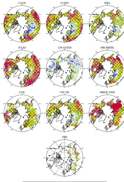
The maps of the 1T vs. dsnow correlations in winter (Fig. 3) demonstrate a pronounced spatial variability in the
1T vs.dsnow relationship. The highest positive correlation occurs in the region of eastern Siberia and the Siberian High-lands. In other regions, namely Scandinavia, the western Russian Arctic, West Siberian Plain and Central Siberian Plateau, the correlation is much weaker and often not sta-tistically significant. These regions have snow (Sect. 4.1.2) influenced by North Atlantic cyclonic activity which brings relatively warm moist air and heavy precipitation in winter (and a positive correlation betweendsnow andTair), leading to relatively small mean1T.
Figure 4.Variation of soil temperature at 20 cm depth (◦C) with air temperature (◦C) for winter 1980–2000. The dots represent the medians of 5◦C air temperature bins and the upper and lower bars indicate the 25th and 75th percentiles, calculated from all Russian station grid points (n=268) and 21 individual winters. The num-bers in each model panel indicate the RMSE between the observed and modelled relationship. Colours represent different snow depth regimes.
3.2 Variability of soil temperature with air temperature and snow depth
Next we assess whether or not the models can correctly re-produce the interannual near-surface soil temperature (Tsoil) variability in relation to snow depth (dsnow)and near-surface air temperature (Tair)variability. Previous studies have noted that the strength of the relationship betweenTsoil andTairis modulated bydsnowand the snow insulation effect increases only up to a limiting depth beyond which extra snow makes little difference to soil temperatures (Smith and Riseborough, 2002; Sokratov and Barry, 2002; Zhang, 2005; Lawrence and Slater, 2010). Zhang (2005) reported that the limiting snow depth is approximately 40 cm.
To inspect the difference in insulation capacity for shallow and thick snow, we investigate theTsoil vs.Tairrelationship under shallow (dsnow≤20 cm) and thick (dsnow≥45 cm) snow conditions. Our Russian observation analysis (Fig. 4,
Figure 5.Variation of soil temperature at 20 cm depth (◦C;yaxis) with snow depth (cm) for winter 1980–2000. The dots represent the medians of 5 cm snow depth bins and the upper and lower bars indi-cate the 25th and 75th percentiles, calculated from all Russian sta-tion grid points (n=268) and 21 individual winters. The numbers in each model panel indicate the RMSE between the observed and modelled relationship. Colours represent different air temperature regimes.
Table 2) indicate a regression slope between Tsoil andTair (0.62◦C◦C−1,R2=0.8) that is 3 times higher under shal-low snow pack than thicker snow conditions (0.21◦C◦C−1,
R2=0.4). This is consistent with observations that the mean freezing n-factor (the ratio of freezing degree days at the ground surface to air freezing degree days) is high at sites where the snow cover is thin or absent and low at sites where the snow cover is thick (e.g. for Yukon in Canada; Karunaratne and Burn, 2003).
Figure 4 clearly shows that some models (CoLM, CLM45, JULES) can capture this difference well. Their regression slopes for thick and thin snow are well separated and in agreement with those from the observed relationship (Ta-ble 2). The RMSE of their modelledTsoil vs.Tair relation-ships from observations is smaller than 4◦C. These mod-els better reproduce the observed1T vs.dsnowrelationship. Other models (LPJ-GUESS, MIROC-ESM, ORCHIDEE) do not reproduce the much greater regression slope between
observations show. They also produce a regression slope for thick snow which is more than twice as large as for the ob-servations. Two models (ISBA, UVic) do not show any sen-sitivity in theTsoilvs.Tairrelation to snow conditions (Fig.4, Table 2). Another measure quantitatively confirms the same models behaviour: the observed averagedsnowin the shallow snow regime is 13.7 cm and that for the thick snow regime is 58.5 cm, so we would expect, if near-surfaceTairand con-ductivities were equal in both snow depth classes, that a ra-tio between the slopes for shallow and thick snow would be 4.3. CLM4.5, CoLM and JULES reproduce this observed variation in the Tsoil vs.Tair relation better than others (Ta-ble 2). JULES and CoLM indicate a change of a factor of 4, while CLM4.5 indicates a change of factor of 2. Other models (LPJ-GUESS, MIROC-ESM, ORCHIDEE) underes-timate the increase of the regression slope for decreasing snow depth; they simulate only a factor change of about 1.5. The two models with unrealistic1T vs.dsnowrelationships (ISBA, UVic) also fail in this evaluation of theirTsoilvs.Tair relationship. They simulate a too-strong sensitivity of Tsoil toTair (regression slopes larger than 0.9◦C◦C−1,R2> 0.7; Table 2) that is almost completely independent of the snow depth regimes, particularly in ISBA, which is not consistent with observations. These models’ spatial correlation patterns between Tsoil andTair also differ greatly from the observa-tions and the other models (Fig. S3) and show very high pos-itive correlation (r> 0.8) in most regions, as may be expected from the large regression slope shown in Fig. 4. The RMSE of their modelled Tsoil vs. Tair relationships from observa-tions reaches ca. 10◦C .
TheTsoilvs.dsnowrelationship (Fig. 5) displays the varia-tion ofTsoilwith changing snow depth and emphasises the re-duced sensitivity ofTsoilto snow depth under thick snow con-ditions. With increasingdsnow,Tsoilasymptotically converges towards a value of around 0◦C. Overall, the Russian obser-vations indicate that snow depth above about 80–90 cm has very little additional insulation effect on Tsoil. Most models show consistent results with regard to this aspect, although the interquartile range of Tsoil for specific snow depths is quite large in some models (ISBA, ORCHIDEE, UVic, UW-VIC; Fig. 5). The figure further points to the air temperature dependency of the relation. On average, for a given dsnow, a colderTsoil is observed for colder near-surface air temper-atures, compared with warmer air temperatures. Most mod-els can replicate this effect of air temperature on the Tsoil vs. dsnow relationship, though with differing accuracy. The RMSE between the observed and modelled relationships can reach ca. 10◦C or more (in ISBA, UVic, UW-VIC), particu-larly under cold conditions.
The spatial patterns of the correlation coefficients between
TsoilandTair(Fig. S3) and betweenTsoilanddsnow(Fig. S4) show a relatively large cross-model scatter in many regions. Obvious outliers in the Tsoil vs. Tair correlation maps are ISBA and UVic, which strongly overestimate the correlation (r> 0.9) over most of the Arctic. This indicates an
underes-timated snow insulation effect and confirms the weak insu-lation in both models, which we already discussed based on their underestimated1T (Fig. 1) and weak correlation be-tween1T anddsnow (Fig. 3). Other models (LPJ-GUESS, ORCHIDEE, UW-VIC) also overestimate the correlation in some regions (e.g. western Russian Arctic,r> 0.7). Most of the simulated maps ofTsoil vs.dsnowcorrelation agree with the observations on a strong positive correlation in eastern Siberia. This is a region of relatively shallow snow (10– 40 cm; Fig. 6) and thereTsoil is very sensitive to variations in snow depth (e.g. Romanovsky et al., 2007). Comparing both simulated correlation maps, it is obvious that in this re-gion,Tsoilcorrelates more strongly withdsnowthan withTair, in agreement with the Russian data and earlier studies (Ro-manovsky et al., 2007; Sherstyukov, 2009).
4 Roles of atmospheric forcing and model processes
The cross-model differences in the snow insulation effect, presented by the air temperature–snow depth–soil temper-ature relationships described above, are partially due to the differences in the atmospheric forcing data and also due to differences in the snow and soil physics used in the LSMs. However, because the climate forcing data sets utilised with each model are observation-based (except for MIROC-ESM), obvious outliers in individual model perfor-mance likely indicate poor or deficient physical descriptions of the air–snow–soil relations in that specific LSM.
4.1 Atmospheric forcing and snow depth 4.1.1 Air temperature and precipitation
Both near-surface air temperature (Tair)and precipitation are given by the climate forcing data sets (Table S1) for all models, except for MIROC-ESM, which simulates both. The cross-model differences in forcing Tair are relatively small and the simulated spatial patterns of temperature are very similar (Fig. S5). All forcing data sets are somewhat colder than Russian station data in their grid cells. The biases of winter meanTairrange from−0.8 to−4.7◦C (Table S2), re-flecting biases in the climate forcing data used by the models. In contrast, MIROC-ESM has a positive (mean)Tairbias of
+2.7◦C.
The large-scale patterns of precipitation are similar across the models, but regional differences can be large (Fig. S6). The individual differences in winter precipitation range from
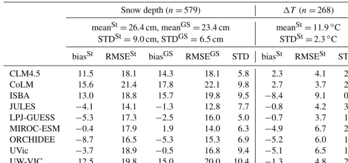
Table 3. Russian station location averaged error statistics for snow depth (cm) and temperature difference between 20 cm soil and air temperature (1T;◦C) for winter 1980–2000. For each variable, the maximum available number of observations (n) is used. MeanSt,GSand STDSt,GSare the observed mean and interannual variability (standard deviation), while STD is the standard deviations of each model. Bias is the mean error “simulation minus observation” and RMSE is the root mean square error. The statistics for snow depth are given based on both station observation (St) and GlobSnow (GS) data.
Snow depth (n=579) 1T (n=268)
meanSt=26.4 cm, meanGS=23.4 cm meanSt=11.9◦C STDSt=9.0 cm, STDGS=6.5 cm STDSt=2.3◦C
biasSt RMSESt biasGS RMSEGS STD biasSt RMSESt STD
CLM4.5 11.5 18.1 14.3 18.1 5.8 2.3 4.1 2.2
CoLM 15.6 21.4 17.8 22.1 9.8 2.7 3.7 2.4
ISBA 13.0 18.8 15.7 19.8 9.5 −8.4 9.1 0.9
JULES −4.1 14.1 −1.3 12.8 7.7 −0.8 4.2 3.2
LPJ-GUESS −5.3 17.3 −2.5 16.0 5.0 −0.7 3.7 1.7
MIROC-ESM −0.4 17.9 1.9 14.0 6.3 −4.9 6.7 2.0
ORCHIDEE −8.7 16.5 −5.3 15.3 6.9 −5.2 6.0 1.9
UVic −3.7 18.9 −0.5 16.8 9.4 −5.1 6.5 1.4
UW-VIC 12.5 19.8 15.0 20.0 10.4 −1.3 4.8 2.1
4.1.2 Snow depth
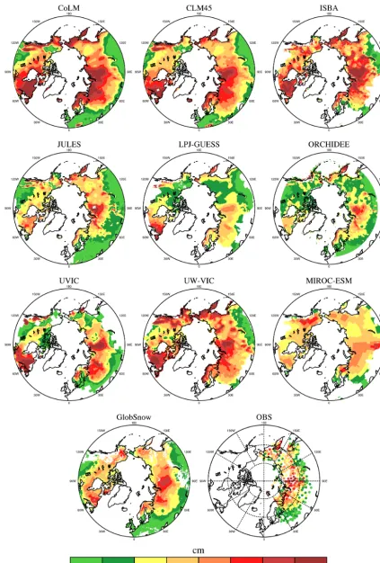
The broad-scale spatial snow depth (dsnow)patterns are sim-ilar across the models and show general agreement with the observed patterns (Fig. 6). The well-pronounced areas of maximum winterdsnow(50–100 cm) are in Scandinavia, the Urals, the West Siberian Plain, Central Siberian Highlands, the Far East, Alaska, Labrador Peninsula and Isle of New-foundland. However, large regional cross-model variability is obvious. Some models (JULES, LPJ-GUESS, ORCHIDEE, UVic) underestimate dsnow, while others (CLM4.5, CoLM, ISBA, UW-VIC) overestimate it (Fig. 6; Table 3). The model biases are quite similar with respect to station observations and GlobSnow data. It should be noted that the models do not account for snowdrift. However, redistribution of snow due to wind is an important aspect, which makes comparison between in situ measured and modelled snow depths difficult (e.g. Vionnet et al., 2013; Sturm and Stuefer, 2013; Gisnas et al., 2014).
Precipitation/snowfall cross-model differences cannot be the primary explanation for these dsnow differences since some models (JULES, MIROC-ESM, ORCHIDEE) have positive bias in precipitation (> 0.2 mm day−1, Table S2) but simulate much lower dsnow compared to other models (Figs. 6, S6, S7, Table 3). Cross-model differences in the interannual variability of winter precipitation do not trans-late simply to corresponding differences in the interannual
dsnowvariability (not shown). For example, UVic calculates the (unrealistically) largest interannual dsnow variability in the boreal European permafrost region, which is not reflected in the precipitation variability. These results indicate that the simulated snow depth is a function of both the prescribed
winter precipitation and the model’s snow energy and water balance.
4.2 Model processes
We have shown that the cross-model spread in the represen-tation of snow insulation effects (Sects. 3.1, 3.2) cannot pre-dominantly be explained by differences in the forcing data (Sect. 4.1), but to a large extent is due to the representation of snow processes in the models. By considering the relation-ship plots (Figs. 1, 4 and 5) and conditional PDFs (Fig. 2), we were able to categorise the models in terms of their snow insulation performance. In this section we discuss the influ-ence of the different snow parameterisations in the models.
Models with better performance (CLM4.5, CoLM, JULES) apply multilayer snow schemes. This allows them to simulate more realistic (stronger) insulation because they consider the snowpack’s vertical structure and variability. They calculate the energy and mass balance in each snow layer, are able to capture nonlinear profiles of snow tem-perature and can also account for thermal insulation within the snowpack such as when the upper layer thermally insu-lates the lower layers (e.g. Dutra et al., 2012). These models also incorporate storage and refreezing of liquid water within the snow and parameterise wet-snow metamorphism, snow compaction and snow thermal conductivity (Table 1), which have been found to be among the most important processes for good snow depth and surface soil temperature simulation (e.g. Wang et al., 2013).
(Table 3, Fig. S8), indicating bias compensation in the two other models. Thus, compensating error effects occur due to snow density and conductivity (Fig. S9, Table 1), which im-pact snow thermal insulation.
Our analysis showed that two models (ISBA, UVic) have
Tsoilvs.Taircorrelation that are too high, indicating that they do not represent the modulation of theTsoilvs.Tair relation-ship by snow depth (Fig. 4). This is consistent with their un-derestimation of1T (Figs. 1, 2, S8, Table 3). In UVic, the snowpack is treated not as a separate layer but as an extension of the top soil layer and a combined surface-to-soil thermal conductivity is calculated (Table 1). Such a scheme largely negates or reduces the insulating capacity of snow (Slater et al., 2001). Koven et al. (2013) noted that such a scheme sim-ulates very little warming of soil and sometimes even cool-ing. The slightly underestimated snow depth (Table 3, Fig. 6) contributes (but not as the primary factor) to reduced snow insulation, as reported for UVic (Avis, 2012).
ISBA strongly underestimates 1T, while strongly over-estimating dsnow, compared with the observations (Table 3, Fig. 6). However, ISBA uses the same atmospheric forcing data as JULES (accordingly the air temperature and pre-cipitation are quite similar; Table S2). Also, the model’s snow density (150–250 kg m−3) is similar to other models (CLM45, CoLM, JULES; Fig. S9) and in agreement with Zhong et al. (2014), who report snow density values of 180– 250 kg m−3 for tundra/taiga and 156–193 kg m−3for alpine snow classes in winter. This apparent contradiction comes from the parameterisation of snow cover fraction within each grid cell (SCF). The version of ISBA used here calculates a unique superficial soil temperature whether or not the soil is covered by snow and all the energy and radiative fluxes are area-weighted by SCF (Eqs. 7 and 20 in Douville et al., 1995). In order to get reasonable albedos in snow-covered forests, as is necessary when ISBA is coupled to the CNRM-CM climate model, the parameterisation gives very low SCF in the boreal forest (between 0.2 and 0.5). Hence, snow in-sulates only 20 to 50 % of the grid cell, despite fairly high snow depths. The heat fluxes from the snow-covered frac-tion are averaged with the fluxes from the snow-free surface, strongly concealing the actual insulating effect of snow and underestimating it over the grid cell. Using the detailed snow model Crocus (Brun et al., 1992; Vionnet et al., 2012) with a SCF equal to 100 % leads to an almost perfect simulation of near-surface soil temperature over northern Eurasia (Brun et al., 2013). A similar experiment with ISBA and a SCF equal to 100 % (Decharme et al., 2016) leads to good performances showing that the low1T in ISBA, despite high snow depth in the present study, is mostly due to this subgrid snow frac-tion. Decharme et al. (2016) still showed that the ISBA re-sults are further improved by updating the snow albedo and snow densification parameterisation.
Interestingly, the ORCHIDEE performance in simulating snow depth and1T is similar to UVic (underestimation of
dsnow and1T; Table 3). However, ORCHIDEE can better
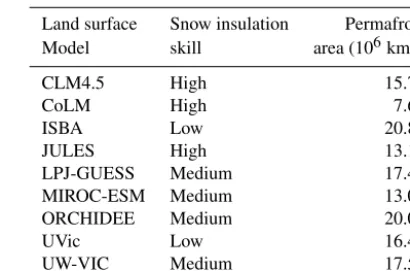
Table 4.Permafrost area, defined as maximum seasonal active layer thickness < 3 m in 1960 (Mc Guire et al., 2016). The IPA map es-timate is 16 million km2(Brown et al., 1997; Slater and Lawrence, 2013).
Land surface Snow insulation Permafrost Model skill area (106km2)
CLM4.5 High 15.77
CoLM High 7.62
ISBA Low 20.86
JULES High 13.19
LPJ-GUESS Medium 17.41
MIROC-ESM Medium 13.02
ORCHIDEE Medium 20.01
UVic Low 16.47
UW-VIC Medium 17.56
represent the observedTsoilvs.Tairrelationship and its mod-ulation due to the snow pack. ORCHIDEE employs, simi-larly to UVic, a fixed snow density and thermal conductivity. However, in contrast to UVic, ORCHIDEE applies a multi-layer scheme and simulates heat diffusion in the snowpack in up to seven discrete layers (Table 1; Koven et al., 2009). This helps to resolve the snow thermal gradients between the top and the base of the snow cover and might explain how some of the snow insulation effects are reasonably represented in ORCHIDEE, despite the simpler treatment of temperature diffusion.
5 Permafrost area
(20.86 million km2). This is inconsistent with previous stud-ies (e.g. Vavrus, 2007; Koven et al., 2013), which concluded that the first-order control on modelled near-surface per-mafrost distribution is the representation of the air-to-surface soil temperature difference. Table 4 shows that the situa-tion is more complex and that snow insulasitua-tion simulasitua-tion is not the dominant factor in a good permafrost extent simula-tion. When the land surface models with poor snow models are eliminated, the remaining models’ simulated permafrost area show little or no relationship with the performance of the snow insulation component, because several other fac-tors such as differences in the treatment of soil organic mat-ter, soil hydrology, surface energy calculations, model soil depth and vegetation also provide important controls on the simulated permafrost distribution (e.g. Marchenko and Et-zelmüller, 2013).
6 Summary and conclusions
The aim of this work was to evaluate how state-of-the-art LSMs capture the observed relationship between winter near-surface soil and air temperatures (Tsoil,Tair)and their mod-ulation by snow depth (dsnow)and climate regime. We pre-sented some benchmarks to evaluate model performance. The presented relation diagrams of Tsoil and the difference betweenTsoilandTairregarding snow depth allow for a much better assessment, used to reveal structural issues of the mod-els, than a direct point-by-point comparison with station ob-servations. The results are based on the comparison of LSMs with a comprehensive Russian station data set.
We see large differences across the models in their mean air–soil temperature difference (1T ) of 3 to 14◦C, in the sensitivity of near-surface soil temperature to air tempera-ture (Tsoil vs. Tair; 0.49 to 0.96◦C◦C−1 for shallow snow, 0.13 to 0.93◦C◦C−1 for thick snow) and in the increase of 1T with increasing snow depth (modal value of 1T
PDF: 0 to 10◦C for shallow snow, 5 to 21◦C for thick snow). Most of the nine models compare to the observa-tions reasonably well (observaobserva-tions:1T =12◦C, modal1T
values of 5◦C for shallow snow and of 14◦C for thick snow, Tsoil vs. Tair=0.62◦C◦C−1 for shallow snow, Tsoil vs.Tair=0.21◦C◦C−1for thick snow). Several models also capture the modulation by air temperature condition (larger increase in 1T with increasing dsnow under colder condi-tions) and display the control of snow depth onTsoil(weaker
Tsoil vs. Tair relationship under thicker snow). However, while they generally capture these observed relationships, their strength can differ in the individual models. Two mod-els (ISBA, UVic) show the largest deficits in snow insulation effects and cannot separate the1Tregimes neither for differ-ent snow depths nor for differdiffer-ent air temperature conditions. This study uses the ensemble of models to document model performance with respect to theTsoilvs.Tair relation-ship, and to identify those with better performance, rather
than to quantify the best model. We were able to attribute performance strength/weakness to snow model features and complexity. Models with better performance apply multi-layer snow schemes and consider complex snow processes (e.g. storage and refreezing of liquid water within the snow, wet snow metamorphism, snow compaction). Those mod-els which show limited skill in snow insulation representa-tion (underestimated1T, very weak dependency of1T on
dsnow, almost unity ratio ofTsoilvs.Tair)have some deficien-cies or oversimplification in the simulation of heat transfer in snow and soil layer, particularly in the representation of snow depth and density (conductivity). We also emphasise that compensation of errors in snow depth and conductiv-ity can occur. For example, an excessive correlation between
Tsoil and Tair can be attributed to excessively high thermal conductivity even when the snow depth is correctly (or over-) simulated. This finding underscores the need for detailed model evaluations using multiple independent performance metrics to ensure that the models get the right functionality for the right reason. It should be noted that the treatment of ground properties, particularly soil organic matter and soil moisture/ice content, also affect the simulated winter ground temperatures. The specific evaluation of these individual pro-cesses is more robustly investigated with experiments con-ducted for individual models (e.g. recently, Wang et al., 2013; Gubler et al., 2013; Decharme et al., 2016).
Snow and its insulation effects are critical for accurately simulating soil temperature and permafrost at high latitudes. The simulated near-surface permafrost area varies greatly across the nine models (from 7.62 to 20.86 million km2). However, it is hard to find a clear relationship between the performance of the snow insulation in the models and the simulated area of permafrost, because several other fac-tors (e.g. related to soil depth and properties and vegetation cover) also control the simulated permafrost distribution.
7 Data availability
The data will be made available through the National Snow and Ice Data Center (NSIDC; http://nsidc.org); the contact person is Kevin Schaefer ([email protected]).
The Supplement related to this article is available online at doi:10.5194/tc-10-1721-2016-supplement.
Acknowledgements. This study was supported by the Permafrost Carbon Vulnerability Research Coordination Network, which is funded by the US National Science Foundation (NSF). Any use of trade, firm, or product names is for descriptive purposes only and does not imply endorsement by the US Government. Eleanor J. Burke was supported by the Joint UK DECC/Defra Met Office Hadley Centre Climate Program (GA01101). Eleanor J. Burke, Shushi Peng, Philippe Ciais and Gerhard Krinner were supported by the European Union Seventh Framework Program (FP7/2007-2013) under grant agreement no. 282700. Theodore J. Bohn was supported by grant 1216037 from the NSF Science, Engineering and Education for Sustainabil-ity (SEES) Post-Doctoral Fellowship program. Bertrand Decharme, Ramdane Alkama and Christine Delire were supported by the French Agence Nationale de la Recherche under agreement ANR-10-CEPL-012-03. This research was sponsored by the integrated approaches and impacts, China Global Change Program (973 Project), National Basic Research Program of China Grant 2015CB953602 and the National Natural Science Foundation of China Grant 40905047. We also thank the editor and reviewers for their comments which improved the manuscript.
Edited by: J. Boike
Reviewed by: two anonymous referees
References
Anderson, E. A.: A point energy and mass balance model of a snow cover, Office of Hydrology, National Weather Service, Sil-ver Spring, Maryland, NOAA Technical Report NWS 19, 1976. Andreadis, K., Storck, P., and Lettenmaier, D. P.: Modeling snow
accumulation and ablation processes in forested environments, Water Resour. Res., 45, W05429, doi:10.1029/2008WR007042, 2009.
Anisimov, O. A. and Sherstiukov A. B.: Evaluating the effect of environmental factors on permafrost factors in Russia, Earth’s Cryosphere, 90–99, 2016.
Avis, C. A.: Simulating the present-day and future distribution of permafrost in the UVic Earth System Climate Model, Disserta-tion, University of Victoria, Canada, 274 pp., 2012.
Bartlett, P. A., MacKay, M. D., and Verseghy, D. L.: Modified snow algorithms in the Canadian Land Surface Scheme: model runs and sensitivity analysis at three boreal forest stands, Atmos. Ocean, 44, 207–222, 2006.
Best, M. J., Pryor, M., Clark, D. B., Rooney, G. G., Essery, R. L. H., Ménard, C. B., Edwards, J. M., Hendry, M. A., Porson, A., Gedney, N., Mercado, L. M., Sitch, S., Blyth, E., Boucher, O., Cox, P. M., Grimmond, C. S. B., and Harding, R. J.: The Joint UK Land Environment Simulator (JULES), model description – Part 1: Energy and water fluxes, Geosci. Model Dev., 4, 677–699, doi:10.5194/gmd-4-677-2011, 2011.
Boone, A. and Etchevers, P.: An intercomparison of three snow schemes of varying complexity coupled to the same land-surface model: Local scale evaluation at an Alpine site, J. Hydrometeo-rol., 2, 374–394, 2001.
Brown, J., Ferrians, O. J., Heginbottom, J. A., and Melnikov, S. E.: International Permafrost Association Circum-Arctic Map of Permafrost and Ground Ice Conditions, scale 1 : 10 000 000,
Circum-Pacific Map Series, USGS Circum-Pacific Map Series, 45 pp., 1997.
Brun, E., David, P., Sudul, M., and Brunot, G.: A numerical model to simulate snow cover stratigraphy for operational avalanche forecasting, J. Glaciol., 38, 13–22, 1992.
Brun, E., Vionnet, V., Boone, A., Decharme, B., Peings, Y., Valette, R., Karbou, F., and Morin, S.: Simulation of northern Eurasian local snow depth, mass and density using a detailed snowpack model and meteorological reanalysis, J. Hydrometeorol., 14, 203–214, doi:10.1175/jhm-d-12-012.1, 2013.
Cook, B. I., Bonan, G. B., Levis, S., and Epstein, H. E.: The thermo-insulation effect of snow cover within a climate model, Clim. Dynam., 31, 107–124, doi:10.1007/s00382-007-0341-y, 2008. Dai, Y., Zeng, X., Dickinson, R. E., Baker, I., Bonan, G. B.,
Bosilovich, M. G., Denning, A. S., Dirmeyer, P. A., Houser, P. R., Niu, G., Oleson, K. W., Schlosser, C. A., and Yang, Z.: The Common Land Model (CLM), B. Am. Meteorol. Soc., 84, 1013– 1023, doi:10.1175/BAMS-84-8-1013, 2003.
Dankers, R., Burke, E. J., and Price, J.: Simulation of permafrost and seasonal thaw depth in the JULES land surface scheme, The Cryosphere, 5, 773–790, doi:10.5194/tc-5-773-2011, 2011. Decharme, B., Brun, E., Boone, A., Delire, C., Le Moigne, P.,
and Morin, S.: Impacts of snow and organic soils parameteri-zation on northern Eurasian soil temperature profiles simulated by the ISBA land surface model, The Cryosphere, 10, 853–877, doi:10.5194/tc-10-853-2016, 2016.
Douville, H., Royer, J. F., and Mahfouf, J. F.: A new snow parame-terization for the Meteo-France climate model, Part 1: Validation in stand-alone experiments, Clim. Dynam., 12, 21–35, 1995. Dutra, E., Viterbo, P., Miranda, P. M. A., and Balsamo, G.:
Com-plexity of snow schemes in a climate model and its impact on surface energy and hydrology, J. Hydrometeorol., 13, 521–538, doi:10.1175/jhm-d-11-072.1, 2012.
Dutra, E., Balsamo, G., Viterbo, P., Miranda, P. M. A., Beljaars, A., Schär, C., and Elder, K.: An improved snow scheme for the ECMWF land surface model: description and offline validation, J. Hydrometeorol., 11, 899–916, 2010.
Essery, R., Morin, S., Lejeune, Y., and Ménard, C. B.: A comparison of 1701 snow models using observations from an alpine site, Adv. Water Resour., 55, 131–148, doi:10.1016/j.advwatres.2012.07.013, 2013.
Essery, R. L. H., Rutter, N., Pomeroy, J., Baxter, R., Staehli, M., Gustafsson, D., Barr, A., Bartlett, P., and Elder, K.: SnowMIP2: An evaluation of forest snow process simulations, B. Am. Meteo-rol. Soc., 90, 1120–1135, doi:10.1175/2009BAMS2629.1, 2009. Ge, Y. and Gong, G.: Land surface insulation response to snow depth variability, J. Geophys. Res., 115, D08107, doi:10.1029/2009JD012798, 2010.
Gerten, D., Schaphoff, S., Haberlandt, U., Lucht, W., and Sitch, S.: Terrestrial vegetation and water balance: Hydrological evaluation of a dynamic global vegetation model, J. Hydrol., 286, 249–270, 2004.
Gisnås, K., Westermann, S., Schuler, T. V., Litherland, T., Isaksen, K., Boike, J., and Etzelmüller, B.: A statistical approach to rep-resent small-scale variability of permafrost temperatures due to snow cover, The Cryosphere, 8, 2063–2074, doi:10.5194/tc-8-2063-2014, 2014.
insulat-ing properties of snow affect soil carbon distribution in the continental pan-Arctic area, J. Geophys. Res., 117, G02020, doi:10.1029/2011JG001916, 2012.
Gubler, S., Endrizzi, S., Gruber, S., and Purves, R. S.: Sensi-tivities and uncertainties of modeled ground temperatures in mountain environments, Geosci. Model Dev., 6, 1319–1336, doi:10.5194/gmd-6-1319-2013, 2013.
Jafarov, E. E., Nicolsky, D. J., Romanovsky, V. E., Walsh, J. E., Panda, S. K., and Serreze, M. C.: The effect of snow: How to bet-ter model ground surface temperatures, Cold Regions Sci. Tech-nol., 102, 63–77, doi:10.1016/j.coldregions.2014.02.007, 2014. Ji, D., Wang, L., Feng, J., Wu, Q., Cheng, H., Zhang, Q., Yang,
J., Dong, W., Dai, Y., Gong, D., Zhang, R.-H., Wang, X., Liu, J., Moore, J. C., Chen, D., and Zhou, M.: Description and ba-sic evaluation of Beijing Normal University Earth System Model (BNU-ESM) version 1, Geosci. Model Dev., 7, 2039–2064, doi:10.5194/gmd-7-2039-2014, 2014.
Jordan, R.: A one-dimensional temperature model for a snow cover, technical documentation for SNTHERM.89, US Army Cold Re-gions Research and Engineering Laboratory, Hanover, NH, 49 pp., 1991.
Karunaratne, K. C. and Burn, C. R.: Freezing n-factors in discontin-uous permafrost terrain, Takhini River, Yukon Territory, Canada, Proc. 8th Int. Conf. on Permafrost, Zurich, 519–524, 2003. Klehmet, K., Geyer, B., and Rockel, B.: A regional climate model
hindcast for Siberia: analysis of snow water equivalent, The Cryosphere, 7, 1017–1034, doi:10.5194/tc-7-1017-2013, 2013. Koven, C. D., Riley, W. J., and Stern, A.: Analysis of
Per-mafrost Thermal Dynamics and Response to Climate Change in the CMIP5 Earth System Models, J. Climate, 26, 1877–1900, doi:10.1175/JCLI-D-12-00228.1, 2013.
Koven, C., Friedlingstein, P., Ciais, P., Khvorostyanov, D., Krinner, G., and Tarnocai, C.: On the formation of high-latitude soil car-bon stocks: Effects of cryoturbation and insulation by organic matter in a land surface model, Geophys. Res. Lett., 36, L21501, doi:10.1029/2009GL040150, 2009.
Langer, M., Westermann, S., Heikenfeld, M., Dorn, W., and Boike, J.: Satellite-based modeling of permafrost temperatures in a tundra lowland landscape, Remote Sens. Environ., 135, 12–24, doi:10.1016/j.rse.2013.03.011, 2013.
Lawrence, D. M. and Slater, A. G.: The contribution of snow condi-tion trends to future ground climate, Clim. Dynam., 34, 969–981, doi:10.1007/s00382-009-0537-4, 2010.
Marchenko, S. and Etzelmüller, B.: Permafrost: Formation and Distribution, Thermal and Mechanical Properties, 8, Academic Press, San Diego, 202–222, 2013.
McGuire, A. D., Koven, C., Lawrence, D. M., Clein, J. S., Xia, J., Beer, C., Burke, E., Chen, G., Chen, X., Delire, C., Jafarov, E., MacDougall, A. H., Marchenko, S., Nicolsky, D., Peng, S., Rinke, A., Saito, K., Zhang, W., Alkama, R., Bohn, T. J., Ciais, P., Decharme, B., Ekici, A., Gouttevin, I., Hajima, T., Hayes, D. J., Ji, D., Krinner, G., Lettenmaier, D. P., Luo, Y., Miller, P. A., Moore, J. C., Romanovsky, V., Schädel, C., Schaefer, K., Schuur, E. A. G., Smith, B., Sueyoshi, T., and Zhuang, Q.: A model-based analysis of the vulnerability of carbon in the permafrost region between 1960 and 2009, Global Biogeochem. Cy., 30, 1– 23, doi:10.1002/2016GB005405, 2016.
Meissner, K. J., Weaver, A. J., Matthews, H. D., and Cox, P. M.: The role of land-surface dynamics in glacial inception: A study
with the UVic earth system model, Clim. Dynam., 21, 515–537, 2003.
Morse, P. D., Burn, C. R., and Kokelj, S. V.: Influence of snow on near-surface ground temperatures in upland and alluvial environ-ments of the outer Mackenzie Delta, Northwest Territories, Can. J. Earth Sci., 49, 895–913, doi:10.1139/E2012-012, 2012. Muskett, R.: Remote sensing, model-derived and ground
measure-ments of snow water equivalent and snow density in Alaska, Int. J. Geosci., 3, 1127–1136, doi:10.4236/ijg.2012.35114, 2012. Nicolsky, D. J., Romanovsky, V. E., Alexeev, V. A., and Lawrence,
D. M.: Improved modelling of permafrost dynamics in a GCM land-surface scheme, Geophys. Res. Lett., 34, L08501, doi:10.1029/2007GL029525, 2007.
Oleson, K. W., Lawrence, D. M., Bonan, G. B., Drewniak, B., Huang, M., Koven, C. D., Levis, S., Li, F., Riley, W. J., Subin, Z. M., Swenson, S. C., Thornton, P. E., Bozbiyik, A., Fisher, R., Kluzek, E., Lamarque, J.-F., Lawrence, P. J., Leung, L. R., Lipscomb, W., Muszala, S., Ricciuto, D. M., Sacks, W., Sun, Y., Tang, J., and Yang, Z.-L.: Technical description of version 4.5 of the Community Land Model (CLM), NCAR Technical Note NCAR/TN-503+STR, doi:10.5065/D6RR1W7M, 2013. PaiMazumder, D., Miller, J., Li, Z., Walsh, J. E., Etringer, A.,
Mc-Creight, J., Zhang, T., and Mölders, N.: Evaluation of Commu-nity Climate System Model soil temperatures using observations from Russia, Theor. Appl. Climatol., 94, 187–213, 2008. Park, H., Fedorov, A. N., Zheleznyak, M. N., Konstantinov, P.
Y., and Walsh, J. E.: Effect of snow cover on pan-Arctic permafrost thermal regimes, Clim. Dynam., 44, 2873–2895, doi:10.1007/s00382-014-2356-5, 2015.
Park, H., Sherstiukov, A. B., Fedorov, A. N., Polyakov, I. V., and Walsh, J. E.: An observation-based assessment of the influences of air temperature and snow depth on soil temperature in Russia, Environ. Res. Lett., 9, 1–7, doi:10.1088/1748-9326/9/6/064026, 2014.
Pavlov, A. V. and Malkova, G. V.: Small-scale mapping of trends of the contemporary ground temperature changes in the Russian North, Earth’s Cryosphere, 13, 32–39, 2009.
Peng, S., Ciais, P., Krinner, G., Wang, T., Gouttevin, I., McGuire, A., Lawrence, D., Burke, E., Chen, X., Decharme, B., Koven, C., MacDougall, A., Rinke, A., Saito, K., Zhang, W., Alkama, R., Bohn, T. J., Delire, C., Hajima, T., Ji, D., Lettenmaier, D. P., Miller, P. A., Moore, J. C., Smith, B., and Sueyoshi, T.: Simulated high-latitude soil thermal dynamics during the past four decades, The Cryosphere, 10, 1–14, doi:10.5194/tc-10-1-2016, 2015. Rawlins, M. A., McGuire, A. D., Kimball, J. S., Dass, P., Lawrence,
D., Burke, E., Chen, X., Delire, C., Koven, C., MacDougall, A., Peng, S., Rinke, A., Saito, K., Zhang, W., Alkama, R., Bohn, T. J., Ciais, P., Decharme, B., Gouttevin, I., Hajima, T., Ji, D., Krinner, G., Lettenmaier, D. P., Miller, P., Moore, J. C., Smith, B., and Sueyoshi, T.: Assessment of model estimates of land-atmosphere CO2 exchange across Northern Eurasia, Biogeo-sciences, 12, 4385–4405, doi:10.5194/bg-12-4385-2015, 2015. Romanovsky, V. E., Sazonova, T. S., Balobaev, V. T., Shender, N.
I., and Sergueev, D. O.: Past and recent changes in air and per-mafrost temperatures in eastern Siberia, Global Planet. Change, 56, 399–413, doi:10.1016/j.gloplacha.2006.07.022, 2007. Saha, S., Rinke, A., Dethloff, K., and Kuhry, P.: Influence of
Schaefer, K., Zhang, T., Bruhwiler, L., and Barrett, A. P.: Amount and timing of permafrost carbon release in response to cli-mate warming, Tellus B, 63, 165–180, doi:10.1111/j.1600-0889.2011.00527.x, 2011.
Schuur, E. A. G., Bockheim, J., Canadell, J. G., Euskirchen, E., Field, C. B., Goryachkin, S. V., Hagemann, S., Kuhry, P., Lafleur, P. M., Lee, H., Mazhitova, G., Nelson, F. E., Rinke, A., Ro-manovsky, V. E., Shiklomanov, N., Tarnocai, C., Venevsky, S., Vogel, J. G., and Zimov, S. A.: Vulnerability of permafrost car-bon to climate change: Implications for the global carcar-bon cycle, Bioscience, 58, 701–714, doi:10.1641/b580807, 2008.
Sherstiukov A.: Climate Change and its Impacts in the Permafrost Zone of Russia, RIHMI-WDC, Obninsk, 127 pp., 2009. Sherstiukov, A.: Dataset of daily soil temperature up to 320 cm
depth based on meteorological stations of Russian Federation, RIHMI-WDC, 176, 224–232, 2012a.
Sherstiukov, A.: Statistical quality control of soil temperature dataset, RIHMI-WDC, 176, 224–232, 2012b.
Singh, V. P., Singh, P., and Haritashya, U.: Encyclopedia of snow, ice and glaciers, Springer, 1240 pp., 2011.
Slater, A. G., Schlosser, C. A., and Desborough, C. E.: The repre-sentation of snow in land-surface schemes: Results from PILPS 2(d), J. Hydrometeorol., 2, 7–25, 2001.
Slater, A. and Lawrence, D.: Diagnosing present and future permafrost from climate models, J. Climate, 26, 5608–5623, doi:10.1175/JCLI-D-12-00341.1, 2013.
Smith, M. W. and Riseborough, D. W.: Climate and the limits of per-mafrost: a zonal analysis, Permafrost Periglac. Process., 13, 1– 15, doi:10.1002/ppp.410, 2002.
Sokratov, S. A. and Barry, R. G.: Intraseasonal variation in the thermoinsulation effect of snow cover on soil tempera-tures and energy balance, J. Geophys. Res., 107, D104093, doi:10.1029/2001JD000489, 2002.
Sturm, M. and Stuefer, S.: Wind-blown flux rates derived from drifts at arctic snow fences, J. Glaciol., 59, 21–34, 2013.
Swenson, S. C. and Lawrence, D. M.: A new fractional snow-covered area parameterization for the Community Land Model and its effect on the surface energy balance, J. Geophys. Res., 117, D21107, doi:10.1029/2012JD018178, 2012.
Takala, M., Luojus, K., Pulliainen, J., Derksen, C., Lemmetyinen, J., Karna, J. P., Koskinen, J., and Bojkov, B.: Estimating Northern Hemisphere snow water equivalent for climate research through assimilation of space-borne radiometer data and ground-based measurements, Remote Sens. Environ., 115, 3517–3529, 2011.
Vavrus, S. J.: The role of terrestrial snow cover in the climate sys-tem, Clim. Dynam., 20, 73–88, doi:10.1007/s00382-007-0226-0, 2007.
Vionnet, V., Brun, E., Morin, S., Boone, A., Faroux, S., Le Moigne, P., Martin, E., and Willemet, J.-M.: The detailed snowpack scheme Crocus and its implementation in SURFEX v7.2, Geosci. Model Dev., 5, 773–791, doi:10.5194/gmd-5-773-2012, 2012. Vionnet, V., Guyomarch, G., Martin, E., Durand, Y., Bellot, H., Bel,
C., and Puglièse, P.: Occurrence of blowing snow events at an alpine site over a 10-year period: observations and modelling, Adv. Water Resour., 55, 53–63, 2013.
Von Storch, H. and Zwiers, F. W.: Statistical Analysis in Cli-mate Research, Cambridge University Press, Cambridge, 484 pp., 1999.
Wang, T., Ottle, C., Boone, A., Ciais, P., Brun, E., Morin, S., Krinner, G., Piao, S., and Peng, S.: Evaluation of an improved intermediate complexity snow scheme in the OR-CHIDEE land surface model, J. Geophys. Res., 118, 6064–6079, doi:10.1002/jgrd.50395, 2013.
Wania, R., Ross, I., and Prentice, I. C.: Integrating peat-lands and permafrost into a dynamic global vegetation model: 2. Evaluation and sensitivity of vegetation and car-bon cycle processes, Global Biogeochem. Cy., 23, GB3015, doi:10.1029/2008GB003413, 2009.
Woo, M., Heron, R., Marsh, P., and Steer, P.: Compari-son of weather station snowfall with winter snow accumu-lation in high arctic basins, Atmos. Ocean, 21, 312–325, doi:10.1080/07055900.1983.9649171, 1983.
Zhang, T.: Influence of the seasonal snow cover on the ground thermal regime: An overview, Rev. Geophys., 43, RG4002, doi:10.1029/2004RG000157, 2005.
Zhang, T., Osterkamp, T. E., and Stamnes, K.: Influence of the depth hoar layer of the seasonal snow cover on the ground thermal regime, Water Resour. Res., 32, 2075–2086, doi:10.1029/96WR00996, 1996.