www.atmos-meas-tech.net/10/15/2017/ doi:10.5194/amt-10-15-2017
© Author(s) 2017. CC Attribution 3.0 License.
Open-loop GPS signal tracking at low elevation
angles from a ground-based observation site
Georg Beyerle and Florian Zus
GFZ German Research Centre for Geosciences, Potsdam, Germany Correspondence to:Georg Beyerle ([email protected])
Received: 23 February 2016 – Published in Atmos. Meas. Tech. Discuss.: 18 April 2016 Revised: 30 September 2016 – Accepted: 17 November 2016 – Published: 3 January 2017
Abstract.A 1-year data set of ground-based GPS signal ob-servations aiming at geometric elevation angles below +2◦ is analysed. Within the “GLESER” measurement campaign about 2600 validated setting events were recorded by the “OpenGPS” open-loop tracking receiver at an observation site located at 52.3808◦N, 13.0642◦E between January and December 2014. The measurements confirm the feasibility of open-loop signal tracking down to geometric elevation an-gles of−1 to−1.5◦extending the corresponding closed-loop tracking range by up to 1◦. The study is based on the premise that observations of low-elevation events by a ground-based receiver may serve as test cases for space-based radio oc-cultation measurements, even if the latter proceed at a sig-nificantly faster temporal scale. The results support the con-clusion that the open-loop Doppler model has negligible in-fluence on the derived carrier frequency profile for strong signal-to-noise density ratios above about 30 dB Hz. At lower signal levels, however, the OpenGPS receiver’s dual-channel design, which tracks the same signal using two Doppler models differing by 10 Hz, uncovers a notable bias. The re-peat patterns of the GPS orbit traces in terms of azimuth angle reveal characteristic signatures in both signal ampli-tude and Doppler frequency with respect to the topography close to the observation site. Mean vertical refractivity gradi-ents, extracted from ECMWF meteorological fields, correlate weakly to moderately with observed signal amplitude fluctu-ations at geometric elevation angles between +1 and +2◦. Results from multiple phase screen simulations support the interpretation that these fluctuations are at least partly pro-duced by atmospheric multipath; at negative elevation angles diffraction at the ground surface seems to contribute.
1 Introduction
For more than a decade the existing Global Navigation Satellite System (GNSS) infrastructure is exploited in me-teorological applications and climate studies. Ground-based GNSS observations reveal valuable information on the tropo-spheric water vapour content integrated along the signal path (see e.g. Bevis et al., 1994; Braun et al., 2001; Businger et al., 1996; Dick et al., 2001; Emardson et al., 1998; Rocken et al., 1997b; Tregoning et al., 1998; Vedel and Huang, 2004; Ware et al., 1997; Hagemann et al., 2003, and references therein). Furthermore, space-based platforms equipped with GNSS re-ceivers allow for the derivation of vertical profiles of atmo-spheric refractivity, dry pressure and temperature (see e.g. Yunck et al., 2000; Kursinski et al., 2000; Melbourne, 2004, and references therein). GNSS data products derived from these ground-based, as well as space-based, observations are being used by meteorological centres for assimilation into numerical weather prediction models (see e.g. Cucurull et al., 2007; Anthes et al., 2008; Healy and Thepaut, 2006; Liu and Xue, 2014; Macpherson et al., 2008; Poli et al., 2010; Rennie, 2010, and references therein). In addition, climate studies in-creasingly take advantage of validated GNSS and GNSS-RO data sets (see e.g. Foelsche et al., 2011; Ringer and Healy, 2008; Steiner et al., 2011; Gleisner and Healy, 2013; Schmidt et al., 2010; Poli et al., 2010, and references therein).
difficul-ties of retrieving dual-frequency carrier phase data, when the ray tangent point enters the lower troposphere (Rocken et al., 1997a). More specifically, Rocken et al. (1997a) no-ticed a significant negative refractivity bias in the lower tro-posphere at tropical latitudes. At low altitudes the GNSS sig-nals experience multipath beam propagation (see e.g. Gor-bunov, 2002b; Hocke et al., 1999). The resulting optical path length differences lead to signal scintillations and these am-plitude fluctuations increase the probability of an early loss of tracking lock. To address these issues new signal track-ing methods were developed and implemented. Whereas the “fly wheeling” tracking method of JPL’s “Blackjack” GPS receivers mounted on CHAMP and GRACE (Ao et al., 2003; Hajj et al., 2004) showed some progress, significant im-provements with respect to probing of the planetary bound-ary layer (PBL), in particular at low latitudes, were obtained with the introduction and implementation of open-loop (O/L) tracking (or raw-sampling) techniques (see e.g. Sokolovskiy, 2001b; Sokolovskiy et al., 2006; Ao et al., 2009; Bonnedal et al., 2010).
The open-loop signal tracking mode successfully resolves the problem of premature loss of signal in the lower tro-posphere at low latitudes (Sokolovskiy, 2001b; Sokolovskiy et al., 2006). In contrast to closed-loop (C/L) tracking, a re-ceiver operating in open-loop mode partially or completely disregards the tracking loop feedback values from the carrier and code discriminators, but instead steers the correspond-ing numerically controlled oscillators (NCOs) uscorrespond-ing a priori parameters. In the following, these O/L parameters, which are usually derived from an atmospheric climatology, are ferred to as “O/L model”. The time duration, which the re-ceiver operates in open-loop tracking mode, may be con-trolled by predetermined threshold values in terms of tan-gent point altitude, elevation angle and/or signal-to-noise ra-tio (SNR). While these general considerara-tions apply to all open-loop and raw-sampling implementations, the specific realisations vary in detail (see e.g. US patents US6731906 B2 and US6720916 B2).
A key requirement for the adoption of O/L signal track-ing in operational GNSS-RO missions is the insensitivity of derived carrier phase paths and code pseudoranges on the particular choice of O/L model. According to Sokolovskiy (2001b) the requirement is met, provided the true atmo-spheric Doppler profile deviates by not more than half of the sampling frequency from the O/L Doppler model. With a typ-ical sampling rate offs=50 Hz this requirement translates into a maximum frequency deviation of 25 Hz.
Recently, Beyerle et al. (2011) claimed, on the basis of GNSS-RO observations recorded by the “IGOR” receiver aboard the TerraSAR-X spacecraft, that the O/L Doppler model may influence the derived refractivity values for low signal amplitudes below about 25 V/V and potentially con-tribute to the negative refractivity bias. In order to substan-tiate this hypothesis they proposed to track each GNSS-RO signal with two O/L models, separated in frequency
space by a predefined offset. We note, however, that other causes certainly contribute to the observed refractivity bias as well (see e.g. Gorbunov et al., 2015; Sokolovskiy et al., 2010, and references therein). Since IGOR firmware modi-fication aboard TerraSAR is unfeasible, two indirect meth-ods were investigated. First, a measurement campaign was conducted in late 2012 with the GNSS-RO receivers aboard the TerraSAR-X and TanDEM-X satellites recording sig-nals from the same setting GPS satellites, but using dif-ferent O/L models (Zus et al., 2014b). Second, within the framework of the GLESER (GPS low-elevation setting event recorder) measurement campaign a ground-based experi-ment was devised and established at an observation site on the “Albert Einstein” science campus in Potsdam, Germany (52.3808◦N, 13.0642◦E) in December 2010. The GLESER campaign targets signals from GPS satellites at low eleva-tions as they set beyond the horizon at elevation angles be-low+2◦. The measurement hardware, the single-frequency
“OpenGPS” receiver, is an in-house development based on C. Kelley’s “OpenSourceGPS” concept (Kelley, 2002).
The occurrence of multiple signal paths (“multipath”) con-necting transmitter device and receiver instrument distin-guishes ground-based from space-based GPS measurements. Local multipath, caused by signal reflections in the direct vicinity of the receiving antenna, cannot be avoided in most ground-based observations (see e.g. Parkinson and Spilker, 1996; Hofmann-Wellenhof, 1997); on a spaceborne plat-form, however, these local reflections may be eliminated to a large extent by careful spacecraft design and suitable antenna placement (cf. Gaylor et al., 2005). Within the framework of space-based radio occultation the term “multipath” as-sumes an alternative connotation and generally refers to tro-pospheric signal propagation close to the ray tangent point, thousands of kilometres away from the receiver. Local mul-tipath, i.e. reflections in the vicinity surrounding the antenna, can be described using geometric optics (see e.g. Elósegui et al., 1995; Anderson, 2000; Larson et al., 2008); tropo-spheric multipath is a diffraction phenomenon and requires wave optical methods to analyse quantitatively (see e.g. Gor-bunov, 2002a; Sokolovskiy, 2001b; Jensen et al., 2003). In the following, however, we will argue that for elevation an-gles below about+2◦wave optical effects may contribute in ground-based observations as well.
the observation. Here, geometric elevation angle is defined as the line-of-sight elevation angle at the receiver antenna disregarding atmospheric refraction effects. Setting events last for about 10 to 15 min on average; hence their durations are about an order of magnitude longer than typical space-based radio occultation measurements (see, e.g. Kursinski et al., 1997). Even if a ground-based observation does not lend itself to the derivation of bending angle profiles (Zuffada et al., 1999; Haase et al., 2014; Healy, 2002; Sokolovskiy et al., 2001), from the signal tracking perspective we re-gard GLESER observations as useful for investigating open-loop tracking of signals with strongly fluctuating SNR. The present study is restricted to the observation and analysis of setting events; an extension towards rising events, however, is technically feasible and may be considered for future im-plementations.
The paper is sectioned as follows. First, closed-loop and open-loop tracking methods are briefly reviewed and the ca-pabilities of GFZ’s OpenGPS receiver are illustrated with some example profiles. Second, the measurements conducted during the GLESER campaign are introduced, and the data processing algorithms and analysis methods are discussed. In the main section of this paper the measurement results are discussed and put into perspective using results from multi-ple phase screen (MPS) simulations. Finally, the OpenGPS hardware and software are described in the Appendix.
2 Closed-loop and open-loop signal tracking
The GLESER campaign utilises the OpenGPS instrument, a single-frequency 12-channel GPS receiver. Several copies of this device, which is based on C. Kelley’s OpenSourceGPS concept (Kelley, 2002), were built at GFZ and used in various ground-based and airborne GPS measurement campaigns (see e.g. Helm, 2008; Helm et al., 2004). In order to provide a self-consistent description of the OpenGPS instrument and its O/L signal tracking implementation, we begin with a brief review of C/L and O/L tracking techniques.
It is well known that inhomogeneities in the tropospheric water vapour field, in particular at low latitudes, can produce multipath propagation of GNSS signals at low elevation an-gles (see e.g. Gorbunov et al., 2004; Beyerle et al., 2003). Space-based RO observations show that under these con-ditions SNR values exhibit strong fluctuations, which early GNSS-RO receivers were unable to track properly (Rocken et al., 1997a). To address premature signal loss GNSS-RO receiver tracking algorithms based on closed feedback loops were replaced by “open-loop” techniques (see e.g. Sokolovskiy, 2001b; Sokolovskiy et al., 2006; Ao et al., 2009; Bonnedal et al., 2010; Wang et al., 2016). If a receiver operates in open-loop mode the feedback loop is opened and the NCO producing the replica signal is steered (in part or fully) from model parameters. This model takes into account the expected signal dynamics from both, the transmitter and
Input
Average
Average Loop Cos
Sin
Phase
Carrier
Average Input
Average Cos
Sin
In-phase
Quad-phase
Figure 1.Schematic representation of closed-loop (top panel) and open-loop (bottom) carrier signal tracking. In closed-loop mode the input signal is correlated with two replica signals, sin and cos, and the latter is phase-shifted by 90◦with respect to the former. The cor-relation sums are low-pass filtered and the output is examined for phase deviations between input and replica signal. The discrimina-tor adjustments close the feedback loop. Open-loop tracking (bot-tom panel) dispenses with the phase discriminator and the numeri-cally controlled oscillator (NCO) is solely steered from model val-ues (Doppler model). The observed carrier phase finally is assem-bled from the NCO phases and the in-phase and quad-phase corre-lation samples.
receiver orbits, clocks biases and drifts as well as the signal propagation characteristics in the lower troposphere. The lat-ter are typically obtained from an atmospheric climatology (Sokolovskiy, 2001b; Bonnedal et al., 2010).
The schematic in Fig. 1 illustrates the two tracking con-cepts for carrier phase tracking; corresponding considera-tions apply to code tracking as well. In standard C/L track-ing (Fig. 1, top panel) the down-converted input signal (“in-put”) is correlated with two internal replica signals (“sin” and “cos”) generated by the NCO (see e.g. Misra and Enge, 2006). The result is low-pass filtered (represented by the box labelled “average”); the carrier phase discriminator deter-mines phase deviations between the observed and modelled replica and provides appropriate adjustments to the loop fil-ter. The sin and cos replica signals, the latter being phase shifted by a quarter cycle, i.e. 90◦with respect to the former, allow us to distinguish phase advances from phase delays be-tween observed and replica signal. The phase discriminator output is digitally filtered (“loop filter”) to prevent unstable loop behaviour (see e.g. Lindsey and Chie, 1981; Thomas, 1989). The receiver output samples (“carrier phase output”) combine the NCO model phases and the phase residuals from the discriminator to yield the observed carrier phase.
-2 -1 0 1 2
Elevation [degree]
10 15 20 25 30 35 40 45 50
C/N
0
[dB Hz]
Closed-loop Open-loop (+5 Hz) Open-loop (-5 Hz)
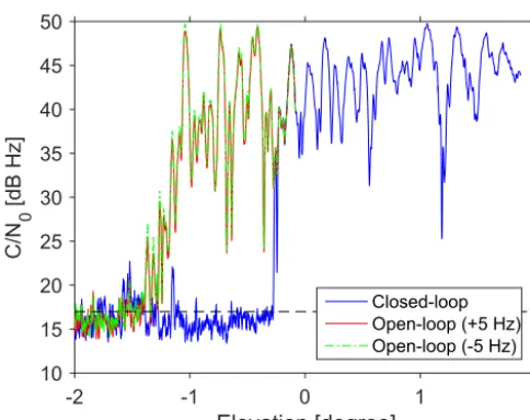
Figure 2.Observed signal-to-noise density ratioC / N0as a func-tion of geometric satellite elevafunc-tion angle. Atmospheric bending amounts to about 1 to 2◦at the observation site and therefore the two open-loop channels (green and red) continue to track the signal down to elevation angles of about−1.2◦. A strong amplitude fluc-tuation at about−0.26◦causes the closed-loop channel (blue) to lose tracking lock much earlier than the open-loop channels (green and red). A C / N0value of about 17 dB Hz is marked in black. Constructive interference produce high C / N0 values exceeding 48 dB Hz at elevations below−1◦. This observation of GPS PRN 7 was recorded on 1 January 2015 between 06:38 and 06:52 GPS time.
noise and proper alignment between replica and observed signal can no longer be maintained. Figure 2 shows exem-plarily the signal-to-noise density ratioC / N0(Badke, 2009; Kaplan, 1996; Parkinson and Spilker, 1996) as a function of geometric elevation angle for a setting event recorded in the morning of 1 January 2015. At elevation angles below about +1.5◦ the density ratiosC / N0start to fluctuate. At about+1.19 and again at+0.56◦transient signal gaps with
C / N0.30 dB Hz occur which last for less than about 0.5 s. During these time intervals the phase discriminator output is dominated by noise, causing enhanced NCO Doppler fre-quency fluctuations as is illustrated in Fig. 3 (blue line). At about−0.26◦elevation low signal level conditions persist for a longer time period and the carrier NCO frequency deviates by hundreds of hertz (blue line in Fig. 3). Correspondingly,
C / N0drops by about 20 dB down to the noise level (Fig. 2) and never recovers during the last part of this setting event.
Open-loop tracking is immune to transient SNR gaps, even if these breaks stretch across extended time periods. The bot-tom panel of Fig. 1 schematically illustrates the concept. In O/L tracking mode the feedback loop is removed and the NCO is solely controlled by model values. The correlation output values, produced by the cos and sin branches, are de-noted by “in-phase” and “quad-phase” correlation samples, respectively (Sokolovskiy, 2001b; Sokolovskiy et al., 2006;
-2 -1 0 1 2
Elevation [deg]
-2000 -1500 -1000 -500 0 500 1000 1500
f NCO
- f
ref
[Hz]
Closed-loop Open-loop (+5 Hz) Open-loop (-5 Hz)
-0.2 -0.1 0 0.1
60 70 80 90 100
Figure 3.Carrier NCO frequency as a function of geometric satel-lite elevation angle. For clarity, a constant frequency value offref= 1.4071 MHz is subtracted. The transition between closed-loop and open-loop tracking is depicted in the insert highlighting the 10 Hz offset between the two O/L channels. Same event as shown in Fig. 2.
Ao et al., 2009; Bonnedal et al., 2010). In low-SNR condi-tions the in-phase and quad-phase samples are dominated by noise. However, since no feedback is present in O/L tracking, these noisy samples cannot produce erroneous control input to the NCO and transient signal gaps do not cause loss of tracking lock as illustrated in Figs. 2 and 3. Red and green lines showC / N0 (Fig. 2) and the NCO carrier frequency (Fig. 3) recorded by the receiver’s two open-loop channels, respectively. In the following the two channels are denoted by the letters A and B. Both channels are attached to the same PRN and therefore track the same transmitter. Their corresponding NCO frequencies are derived from the same model, but on channel A’s value an additional−5 Hz, and on B an additional+5 Hz, is added, resulting in a 10 Hz inter-channel offset. This 10 Hz shift can clearly be identified in Fig. 3 (insert); here, O/L tracking mode starts at an elevation angle of−0.08◦and reaches the nominal 10 Hz shift after a brief initialization phase at−0.13◦elevation.
3 Measurements
receiver malfunctioned due to an operator error and 437 ob-servations from that time period are removed from the data set, leaving 2581 low-elevation events.
The instrument is housed on the top floor of the for-mer water tower on the “Albert Einstein” science cam-pus in Potsdam, Germany (52.3808◦N, 13.0642◦E). An active L1(1575.42 MHz) GPS antenna (NovAtel/ANTCOM 2G15A-XTB) is mounted on the tower’s observation deck and tilted by about 45◦towards the western horizon to in-crease recorded signal strength at very low elevation an-gles. The antenna includes a low-noise amplifier with 33 dB gain and is sensitive to right hand circular polarisation only. A 10 m low-loss signal cable connects the antenna to the OpenGPS receiver. According to the manufacturer’s docu-mentation the cable loss is 14 dB per 100 m at 1 GHz.
Figure 4 depicts the panoramic view of the western hori-zon from the observation deck between azimuth angles of 180 (south) and 360◦(north). The azimuth angles are marked
in black at the top side of the photograph. Thick red lines in-dicate the azimuth angles of those PRNs, which are analysed in the present study. The picture was taken a few metres east of the receiving patch antenna, which is visible to the right of the 290◦azimuth tick mark.
Data acquisition is activated once a satellite enters the ob-servation window which ranges from 200 to 340◦in azimuth (thin broken red lines in Fig. 4) and from+2 to−2◦in ele-vation. Any additional satellite entering the observation win-dow during this time period is disregarded and not tracked in O/L mode. Raw observables stored on disk include pseu-doranges ρC/L,n, carrier phasesϕC/L,nand time tagstn for
all C/L channels. In addition, raw O/L measurements (in-phase and quad-(in-phase correlation sums eIn and Qen; NCO
ranges ρNCO,n and NCO carrier frequencies fNCO,n from
both O/L channels) are written to separate files. Here, the subscriptn=1,2, . . .enumerates the successive TIC events (for an explanation of TIC event, see Appendix A1) recur-ring every 20 ms. The correlation sums eIn andQen are not
sampled at TIC instants but are coherently integrated over a time period of 20 ms preceding the TIC event. The corre-sponding time offset between eIn, Qen andϕNCO,n is
disre-garded in the following analysis. Raw data accumulation rate is about 360 MB day−1or about 2.5 GB week−1.
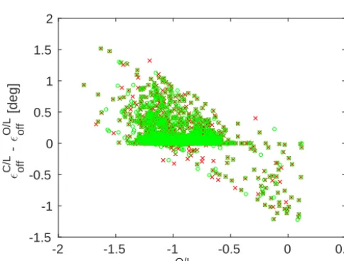
In order to quantify the performance gain of O/L in com-parison to C/L detection we compare in Fig. 5 the lowest elevation angles observed in the two tracking modes, offO/L
and offC/L. They are defined as the minimum elevation in a given setting event with the smoothed density ratio C / N0 still exceeding 30 dB Hz. Smoothing is performed by a run-ning mean filter of 1 s width. We find that out of a total of 2581 setting events 2368 and 2366 were recorded by the O/L channel A and B, respectively. In the remaining 8 % of the observations closed-loop tracking stopped too early and O/L was never activated. With active channels A and B, however, in about 86 % of the O/L measurements (2017 out of 2368
and 2069 out of 2366 for channel A and B, respectively) end elevation angles from O/L tracking yielded smaller val-ues compared to the C/L results. Additionally, in 21 % of the measurements (499 out of 2368 and 505 out of 2366 for channel A and B, respectively) O/L tracking extended more than 0.25◦further down than the corresponding C/L obser-vation.
4 Data processing and analysis
Data processing is performed on an event-by-event basis. Typically, setting events last about 700–900 s; however, mea-surements extending over a time period of up to 1400 s are occasionally observed. During the initial stage OpenGPS, raw data files are converted to MATLAB®binary format to facilitate the subsequent processing steps. First, the observed in-phase and quad-phase samples sums are demodulated:
In=DneIn;Qn=DnQen. (1)
This done to allow calculation of the residual phase samples:
ϕres,n=atan2(Qn, In) . (2)
Here, the four-quadrant arctangent atan2(x, y) denotes the principal value of the angle of the complex numberx+i y.
The literature discusses two methods for the determina-tion of the data bitsDn, “internal” and “external”
demodula-tion. On the one hand,Dncan be extracted from the
obser-vationseInandQenthemselves (Sokolovskiy et al., 2009). On
the other hand, external demodulation extractsDnfrom
inde-pendent observations, such as GFZ’s NavBit data base, reg-istered under doi:10.1594/GFZ.ISDC.GNSS/GNSS-GPS-1-NAVBIT (Beyerle et al., 2009). In the following, external de-modulation is used since in low-elevation events the modulus of the difference between adjacent the carrier phase residuals,
ϕres,n−ϕres,n−1
, frequently reaches and exceeds±90◦. In
these cases a clear separation between propagation-induced phase fluctuations and phase changes due to a sign change ofDnis difficult to achieve.
Accumulated residual carrier phase samples8res,n then
follow from
8res, n≡ϕres, n+Cn=atan2(Qn, In)+Cn (3)
with the unwrapping termCndefined by
Cn=
Cn−1+2π atan2(Qn, In)−atan2 Qn−1, In−1
<−π Cn−1−2π atan2(Qn, In)−atan2 Qn−1, In−1
>+π
Cn−1 else
(4)
ifn >1 andCn=1=0 (Beyerle et al., 2011). In addition, dur-ing this first processdur-ing stage the receiver’s 1 Hz navigation solution, which includes an estimate of the receiver’s clock bias, is retrieved as well.
Figure 4.View towards west from the observation platform. The picture was taken about 2–3 m behind the receiver’s GPS antenna, which is tilted by about 45◦towards west (the antenna and its mounting pole is visible at about 290◦azimuth angle). The metal structure at about 220◦is part of a lightning protection system and does not block the antenna’s field of view, which ranges from 200 to 340◦. Throughout the observation period a satellite with a given PRN sets beyond the horizon at almost the same azimuth angle. The angles of those nine PRNs discussed in the present study are marked in red.
offO/L
[deg]
-2 -1.5 -1 -0.5 0 0.5
off
C/L
-
off
O/L
[deg]
-1.5 -1 -0.5 0 0.5 1 1.5 2
Figure 5.Open-loop performance in terms of the gain or loss in el-evation angle range compared to closed-loop tracking. The end ele-vationsOoff/LandC/Loff are defined as the lowest angle withC / N0 still exceeding 30 dB Hz. In general, O/L tracking lowers the final elevation angle by about 0.11◦on average. However, in about 14 % of the measurements C/L tracking outperforms the O/L channels, in a few cases by up to 1◦. Red markers refer to O/L channel A and green to channel B.
the bias-corrected receiver clock time and linearly interpo-lated from 1 to 50 Hz. From the bit-corrected phase sam-ples8res,nthe observed carrier frequencies
fobs(A,B),n ≡fNCO(A,B),n+fres(A,B),n
≈fNCO(A,B)+ 1
2π
8(A,B)res,n −8(A,B)res,n−1
tn−tn−1
(5) are derived with superscriptAandB, indicating the corre-sponding O/L channel. Figure 6 showsfobs(A,B),n (Eq. 5) corre-sponding to the event plotted in Fig. 3 using external data bit demodulation (red and green lines). The C/L channel (blue line) loses lock at about−0.3◦elevation and its carrier fre-quency output leaves the scale. Incidentally, at about−1.2◦
-1.5 -1 -0.5 0 0.5
Elevation [deg]
50 100 150 200
f obs
- f
ref
[Hz]
Closed-loop Open-loop (+5 Hz) Open-loop (-5 Hz)
Figure 6.Observed carrier frequenciesfobs, reconstructed from NCO and residual frequencies (Eq. 5), using external data bit de-modulation as a function of elevation angle (red and green). In ad-dition, the closed-loop result is plotted in blue. For clarity, a con-stant offsetfref=1.4071 MHz is subtracted. Same event as shown in Figs. 2 and 3.
the C/L frequency briefly crosses the displayed frequency range again. Below about−1.2◦elevation Earth’s limb com-pletely shadows the signal from PRN 7 (see Fig. 2) and from there on O/L and C/L outputs contain noise only.
In addition, with the observed in-phase and quad-phase correlation sums,eInandQen(Eq. 1), the signal-to-noise
den-sity ratioC / N0, in units of dB Hz, is calculated according to Badke (2009), Kaplan (1996) and Parkinson and Spilker (1996):
C / N0(dB Hz)=10·log
e I2+Qe2
2·Var QeC/L
·Tc
!
. (6)
Here,hxiis the mean value ofx andTc=0.02 s denotes the coherent integration time. Var QeC/L
mas-ter channel running in C/L mode between 0 and+2◦ eleva-tion angle.
If no GPS signal is present and the receiver input signal is pure noise,eI andQeare uncorrelated and
D e I2+Qe2
E =2·
D e Q2
E
=2·Var Qe
≈2·VarQeC/L
(7) since
e Q=
0. Under these conditions the density ratio
C / N0(dB Hz)decreases to a value of
10·log
1
Tc
≈17 dB Hz (8)
using Eq. (6) (dashed black line in Fig. 2).
5 Simulations
In order to interpret the observedC / N0fluctuations we per-formed a series of MPS simulations (Knepp, 1983; Martin and Flatté, 1988; Grimault, 1998). The propagation of a plane wave through the lower troposphere is modelled by a series of 500 non-equidistant phase screens covering the range from the receiver to a distance of 500 km. On each phase screen the wave suffers a phase delay determined by the inter-screen distance1zand the refractivity height profile (Sokolovskiy, 2001a)
N (h)=400 exp
−h
hs
1−0.052
πatan h−h
tp
hzn
, (9) with height h, scale height hs=8 km, PBL top height htp and PBL top transition zonehzn=50 m. The interaction of the wave with the ground surface is modelled by applying a raised-cosine filter with a 6 dB steepness of 25 m (i.e. within 25 m the filter weight decreases by 6 dB) at zero altitude. The phase screens extend vertically from −20 to +20 km with a 5 km wide raised-cosine filter applied at the upper and lower boundary to suppress spurious diffraction effects; the receiver altitude is taken to be 50 m. The variation of el-evation angle between −2 and +2◦ is modelled by tilting the ground surface and its overlying atmosphere correspond-ingly.
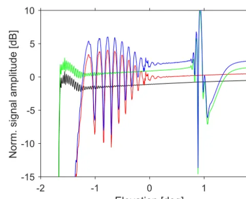
Results from four simulation runs are shown in Fig. 7; it displays the normalised signal amplitude as a function of elevation angle. Signal absorption at the ground surface produces characteristic diffraction patterns for elevation an-gles below 0◦(red and blue lines). Without ground
absorp-tion the diffracabsorp-tion patterns almost disappear and the profiles approximate step functions expected from geometric optics (green and black). The MPS simulations did not produce
C / N0fluctuations for horizontally oriented PBL tops (pa-rameterised by the parameterhtpin Eq. 9). However, if the top layer tilts towards the receiver, substantial signal devi-ations at elevation angles above 0◦ are observed. Figure 7 illustrates this phenomenon for a PBL top layer ascending
-2 -1 0 1 2
Elevation [deg]
-15 -10 -5 0 5 10
Norm. signal amplitude [dB]
Figure 7.Normalised signal amplitudes as a function of elevation angle derived from several MPS simulations. Refractivities on the individual phase screens are calculated from an exponential profile furnished with a planetary boundary layer in the lower troposphere. Signal absorption at the surface is taken into account (red and blue lines); green and black lines show the result without ground ab-sorption. Two boundary layers are modelled: a horizontal boundary layer top at 2 km altitude (red and black) and a layer top increasing from 1 to 2 km between 30 and about 60 km distance from the re-ceiver (blue and green). For legibility the red, green and blue lines are shifted by an additional +1,+2 and+3 dB offset, respectively. For details see text.
from 1 km at 30 to 2 km at about 60 km distance (green and blue lines); at distances below 30 and above 60 kmhtp re-mains fixed at 1 and 2 km, respectively.
The MPS simulation results, plotted in Fig. 7, highlight ground diffraction effects below about 0◦ elevation angle (blue and red) and PBL-induced C / N0 variations above about 0◦ (blue and green). The results suggest that these C / N0fluctuations are independent from each other and tend to be separated in elevation angle space. Finally, we note that the addition of irregularities on spatial scales characteristic for turbulence to the refractivity profiles did not produce sig-nificantC / N0changes.
6 Discussion and interpretation
We begin the discussion of the GLESER results by compar-ing the performance of internal versus external data bit de-modulation and define the quantity as
EnX≡ D
X,int
n −D
X,int
n−1
−
Dextn −Dnext−1
. (10)
Here,|x|denotes the modulus ofx, the superscriptX=Aor
-2 -1 0 1 2 Elevation [deg]
0 0.5 1
(
E
A
+
E
B
) / 2
0 2 4
Number of obs. per bin
×105
Figure 8.Failure rate of internal navigation bit retrieval in terms of averaged performance parameterhEi(Eq. 10) as a function of elevation angle for signal density ratios C / N0≥30 dB Hz (blue, left axis). The corresponding number of observations per elevation bin is plotted as well (red, right axis). The statistics is based on 242 observations recorded in January 2014.
the next, rather than differences between the bit values, since only the former affect the derived carrier frequency. We note thatEnX=1 for randomly chosenDnX,intandDnext.
For 242 observations in January 2014 with signal den-sity ratiosC / N0≥30 dB Hz the parametersEn(Eq. 10) are
grouped into an elevation grid with 0.1◦ bin size and aver-aged. The result is shown in Fig. 8. At elevation angles just below 0◦there is good agreement between internal and
exter-nal data bit retrieval; at lower elevations, however, the failure rate increases significantly. Results for elevation angles be-low−1.2◦are statistically not significant due to the strongly decreasing number of observations (red line). To eliminate potential errors caused by internal data bit removal, we re-strict the following discussion to data processed using exter-nal demodulation.
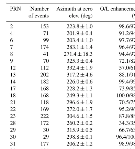
Table 1 lists all 19 PRNs recorded during the 311-day ob-servation period in 2014 and the corresponding number of setting events. The third column gives the mean azimuth an-gle and its 1σ standard deviation at 0◦elevation. Enhanced changes in azimuth angle of PRN 8 are most likely related to the decommissioning of GPS space vehicle number 38 in Oc-tober 2014. The last column in Table 1 shows the fractions of profiles in which O/L tracking reached a lower elevation an-gle than the corresponding C/L result. For example, a value of 70 % indicates that in 30 out of 100 observations the C/L channel tracked to a lower elevation than the corresponding O/L channels. The low O/L enhancement values for PRN 28 might be caused by signal reflections at the water surface of Templiner Lake (see Fig. 4 at about 260◦azimuth angle). As described in the Appendix (Sect. A2), the O/L model is ini-tialised within the elevation angles range between 0 and+2◦.
Table 1.Number of low-elevation events and azimuth angle at zero elevation for all 19 PRNs recorded during 311 days in 2014. Az-imuth angle is given as mean and 1σ standard deviation. The last column lists the percentages of observation in which O/L tracking reached a lower elevation angle than the corresponding C/L detec-tion. The first number refers to O/L channel A, the second to chan-nel B.
PRN Number Azimuth at zero O/L enhancement
of events elev. (deg) (%)
2 153 223.8±1.0 98.6/97.3
4 71 201.9±0.4 91.2/94.1
6 99 203.4±1.0 97.7/97.7
7 174 283.1±1.4 96.4/97.0
8 41 271.4±18.3 94.4/97.2
9 70 325.3±0.4 72.1/82.0
12 112 332.4±1.9 57.0/61.3
13 202 317.2±4.6 88.1/91.7
14 182 226.0±0.6 99.4/99.4
17 168 228.2±1.3 73.9/85.1
18 168 249.3±1.1 100.0/98.8
21 118 296.6±1.9 70.5/75.0
22 169 272.0±1.7 95.2/96.4
23 222 304.6±1.5 87.8/88.2
28 172 260.2±0.2 34.3/35.5
29 30 315.9±0.5 66.7/63.3
30 29 298.8±0.1 96.4/100.0
31 177 206.2±1.2 98.9/98.9
32 224 318.3±1.1 70.3/75.1
It appears feasible that surface reflections induceC / N0 fluc-tuations at these elevation angles (see e.g. Anderson, 2000; Larson et al., 2008), degrading the quality of the O/L model and thereby causing poor O/L performance.
The panorama photograph Fig. 4 shows the view to the lo-cal horizon within the 140◦wide observation window rang-ing from 200 to 340◦ and centred at 270◦ azimuth (west). It exhibits a substantial variation of surface properties in az-imuth angle with enhanced building densities of the city of Potsdam in a westerly to north-westerly direction (about 280 to 350◦), mostly forests at azimuth angles below 270◦ and water surfaces from Templiner Lake between about 250 and 260◦. Also indicated in Fig. 4 are the approximate zero-elevation azimuth angles of setting GPS satellites (red marks). Due to the specific geometry of the GPS constella-tion the orbit traces exhibit a characteristic azimuth angle re-peat pattern when viewed from a fixed ground-based location (Axelrad et al., 2005; Choi et al., 2004), i.e. a specific PRN sets at the same azimuth angle with small deviations of less than 1◦(see centre column of Table 1).
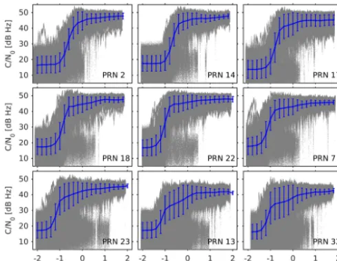
Pots-Figure 9. Carrier signal-to-noise density ratio, averaged over the two O/L channels, as a function of elevation angle. The panels show observations from nine PRNs sorted row-wise according to increas-ing azimuth angle (see Fig. 4). Mean and 1σ standard deviations, calculated from 0.2◦elevation bins, are marked in dark blue. Once the signal is completely blocked by the horizon,C / N0 drops to about 17 dB Hz (see Eq. 8).
dam throughout the year. The non-uniform topography most likely contributes to the observed variability in C / N0 (see e.g. Fig. 2) and, as will be discussed below, Doppler fre-quency with respect to azimuth angle. The occurrence time of the setting event, however, shifts by about 4 min day−1, which corresponds to 24 h per average year (365.25 days). Thus, the statistical analysis performed in the present study essentially averages out any potential diurnal variation. The investigation of these temporal variations is left to future re-search.
Figure 9 provides a general overview of the observed mean signal density ratios
C / N0avg[dB Hz] ≡1
2
C / N0A[dB Hz] +C / N0B[dB Hz]
(11) as a function of elevation angle. We note that by ex-pressing C / N0 in units of dB Hz, Eq. (11) constitutes in effect a geometric mean value in terms of the ratios
e
I2+Qe2 2·Var(QeC/L)·Tc (see Eq. 6). Figure 9 shows C / N0 for PRNs 2, 7, 13, 14, 17, 18, 22, 23 and 32. The following analysis is focused on this set of nine PRNs; they were selected according to data availability and azimuth an-gle coverage. The individual panels in Fig. 9 and the follow-ing figures are arranged row-wise accordfollow-ing to increasfollow-ing az-imuth angle (see Fig. 4). In Fig. 9 also the mean and 1σ stan-dard deviations are plotted with an elevation bin size of 0.2◦ (blue). The overall features are similar in all nine panels with
C / N0≈40–45 dB Hz at the start of the setting event, de-creasing to about 15 dB Hz at the lower end. At about 0◦ elevation, at the transition between C/L and O/L tracking,
-100 0
2
Frq. offset [Hz] 0
Delay [chips] 0.5
0
Norm. correlation
-2 100 1
Figure 10.Normalised C/A code correlation function as a function of delay and Doppler frequency offset. At zero delay the code cor-relation function corresponds to the frequency response (solid red line). It closely matches the modulus of the normalised sinc func-tion (dotted red line, shifted by+2.5 chips for clarity).
signal propagation over the urban area (PRNs 23, 13 and 32 corresponding to azimuth angles of 305, 317 and 318◦) ap-pear to exhibit strongerC / N0attenuations and fluctuations compared to signals arriving from more southerly directions across forest areas.
Examining density ratio averages (Eq. 11) in lieu of
C / N0AandC / N0Bis justified, since the two values agree in the majority of observations. As a matter of principle, how-ever, significant deviations are conceivable, because the den-sity ratio depends on frequency offset1f(A,B) between the O/L NCO frequencyfNCO(A,B) and the signal’s true carrier fre-quencyf0,
1f(A,B)≡fNCO(A,B)−f0. (12)
Provided the observed and replica signal are perfectly aligned in the pseudorange domain, the amplitude loss in-duced by1f(A,B)is given by
L1f(A,B)≡
sin π 1f(A,B)Tc
π 1f(A,B)T
c
(13)
with a coherent integration time ofTc. For illustration Fig. 10 shows the normalised C/A code correlation function as a function of code lag and frequency offset in the vicinity of the correlation maximum and the loss functionL(1f(A,B))
at zero delay (red line).
Thus, in the absence of other factors affectingC / N0Aand
C / N0B individually, the density ratios of channel A and B will differ by
1C / N0≡C / N0A−C / N0B
=20 log
1f(B) 1f(A)
sin π 1f(A)Tc sin π 1f(B)T
c
. (14)
Figure 11.Same as Fig. 9, however, showing1C / N0, the differ-ence of the two O/L density ratios, as a function of elevation angle.
of 0.2◦, are marked in blue with error bars indicating the 1σ
standard deviation. The mean values of 1C / N0 are zero within the statistical uncertainties; individual observations, however, differ by more than 10 dB Hz. While in general the largest deviations occur below 0◦elevation, i.e. during O/L tracking, also C/L tracking results exhibit non-zero values of
1C / N0. Finally, in the panels for PRNs 7, 22 and 23 char-acteristic features between−1 and 0◦elevation are evident. Their most likely explanation are multipath signal propaga-tion at azimuth angles between about 270 and 300◦.
The observed density ratio difference 1C / N0 can be analysed quantitatively. For this purpose the observation
fobs(A,B)≈f0 is assumed to be a valid approximation for the true carrier frequencyf0. Using the defining Eq. (5) we ob-tain
fobs(A)−fobs(B)=fNCO(A) +fres(A)−fNCO(B) +fres(B)≈0 (15) and
1C / N0(fres(A))
≈20 log
fres(A)+10 Hz
fres(A)
sinπ fres(A)Tc
sin
π
fres(A)+10 Hz
Tc
(16)
or, alternatively,
1C / N0
fres(B)
≈20 log
fres(B)
fres(B)−10 Hz sinπ
fres(B)−10 Hz
Tc
sinπ fres(B)Tc
. (17)
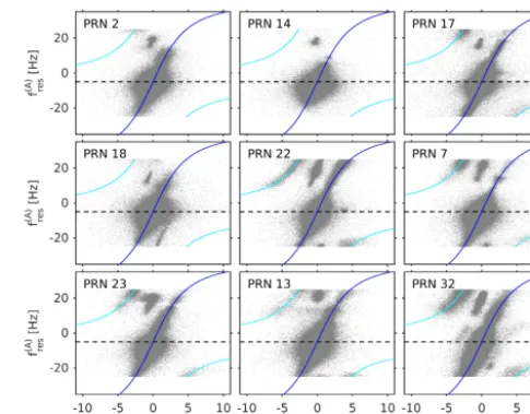
Figure 12 shows the correlation between the observed den-sity ratio differences 1C / N0 andfres(A) (gray data points).
Figure 12.Same as Fig. 9, however, showing the residual frequency in O/L channel A as a function of1C / N0, the difference of the two O/L density ratios (gray points). The theoretically expected result (Eq. 16) is shown in dark blue; light blue lines are the theoretical result shifted by±50 Hz highlighting the occurrence of frequency aliasing. The horizontal dashed lines mark the−5 Hz residual fre-quency.
Here, the data set is restricted to the subset of typically 210 000 (PRN 2) to 370 000 (PRN 7) samples tracked in O/L mode. The expected result derived from Eq. (16) is over-laid in dark blue; dashed lines mark the residual frequency of−5 Hz.
The resulting patterns exhibit a marked dependence on PRN, i.e. on azimuth angle. Whereas the observations of PRN 14 (azimuth angle at about 226◦) indicate only mod-erate excursions in terms of residual frequency with most data points clustered at −5 Hz (dashed line), the signals from PRN 32, arriving from an azimuth angle of 318◦, show strong deviations causing residual frequencies exceeding the Nyquist value offs/2=25 Hz. Here the agreement with the theoretical results (blue line, Eq. 16) is evident. A substan-tial number of observations deviate from the O/L model by more thanfs/2 and are therefore affected by aliasing. The light blue curves, which are derived from Eq. (16) but shifted by±50 Hz, show good agreement with the observations and substantiate this interpretation. The aliasing effect is stronger for negativefres(A)since channel A is shifted with respect to the O/L model by an additional−5 Hz.
Correspondingly, aliasing for positive residual frequencies is stronger for channel B since this channel is shifted with respect to the O/L model by+5 Hz as illustrated by Fig. 13, which shows the corresponding result derived O/L channel B data. Again, the dark blue lines (and the aliased curves in light blue) mark the theoretical result derived from Eq. (17).
The preceding discussion is based on the assumption
Figure 13.Same as Fig. 12, however, showing the corresponding results from O/L channel B.
Figure 14. Same as Fig. 9, however, showing the difference be-tween the two observed frequencies obtained from O/L channel A and B as a function of the mean signal-to-noise density ratio (Eq. 11). Mean and 1σstandard deviations, calculated fromC / N0 bins 2.5 dB Hz wide, are marked in green. The fraction of data points exceeding1fobs>+40 Hz is indicated asρ40 Hz. The re-sult of the statistical analysis excluding this subset still exhibits a positive bias ifC / N0.30 dB Hz (red).
Referring to Fig. 14, however, we deduce that Eq. (18) is not strictly fulfilled, in particular for low signal-to-noise density ratios. The panels of Fig. 14 show the observed frequency difference1fobs≡fobs(A)−fobs(B)as a function of mean den-sity ratio for the selected nine PRNs. Their mean values and 1σstandard deviations, sorted into 2.5 dB Hz bins, are super-imposed on the individual data points (gray dots) as green lines.
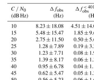
Table 2.Mean and standard deviations of1fobs(centre column) for nine values of the carrier signal-to-noise density ratioC / N0 between 10 and 50 dB Hz; averaging bin size is 5 dB Hz. The statis-tics is based on all PRNs shown in Fig. 14. The third column lists the corresponding result, neglecting frequency deviations larger than 40 Hz.
C / N0 1fobs 1fobs<40 Hz
(dB Hz) (Hz) (Hz)
10 8.23±18.08 4.51±14.01 15 5.48±15.47 1.85±9.68 20 2.75±11.50 0.50±5.68 25 1.28±7.89 0.19±3.29 30 1.23±7.71 0.08±1.96 35 1.39±8.17 0.06±1.38 40 0.95±6.78 0.04±1.12 45 0.62±5.47 0.05±1.28 50 0.56±5.23 0.06±1.68
In all panels a small fraction of the data set, denoted by
ρ40 Hz in Fig. 14, populates the frequency band 1fobs&+ 40 Hz with a mean value of about+50 Hz and signal lev-els ranging from 10–20 dB Hz to more than 40 dB Hz. Again, this+50 Hz offset is caused by aliasing. If the true signal fre-quencyf0occurs within the frequency range between+20 and+25 Hz, it is correctly tracked by channel A but aliased to the−30 to−25 Hz frequency window by channel B, since channel B’s NCO is shifted by−10 Hz with respect to chan-nel A’s NCO and therefore its frequency range extends from
−30 to+20 Hz. Thus, the frequencies observed by channel A and B differ by+50 Hz. Conversely, signals appearing at fre-quencies between−20 and−25 Hz are properly recorded by channel B but suffer aliasing in channel A again, producing a+50 Hz offset in1fobs. Formally, the observed frequency difference1fobsas a function of true frequencyf0is 1fobs(f0)=
fNCO(A) +fres(A)(f0)
−fNCO(B) +fres(B)(f0)
=
0 Hz −20 Hz< f0<+20 Hz
+50 Hz else. (19)
We note that in both cases the offset is+50 Hz and there-fore signals differing fromf0by integer multiples of 50 Hz cannot be distinguished using dual-channel O/L tracking.
Even though the fraction ρ40 Hz remains below 4 %, the corresponding samples bias the mean value (green lines in Fig. 14) towards positive frequencies, but they are not the sole cause for the observed bias. If all observations with
1fobs≥ +40 Hz are removed from the data set, the corre-sponding mean values are still biased, albeit significantly less (red lines in Fig. 14).
The magnitude of the observed frequency bias can be mo-tivated in the following way. In the limit of vanishing signal levels the residual frequencies are dominated by noise and thus
fres(A)≈0≈fres(B). (20)
Under these circumstances the observed frequency differ-ence between channel A and B becomes
lim
C / N0→noise
1f = lim
C / N0→noise
fobs(A)−fobs(B)
=fNCO(A) −fNCO(B) =10 Hz. (21) The mean values observed in Fig. 14 are consistent with this estimate. However, the figure also shows that for C / N0&30 dB Hz the frequency difference 1fobs is bias free; the deviations occur solely at signal levels
C / N0.30 dB Hz. We note that this bias is independent from the sampling frequency fs. The numerical values of C / N0, however, which characterise the transition zone be-tween biased and bias-free samples, depend on the antenna gain and other receiver-specific parameters. They cannot be directly compared to observations from space-based GNSS-RO payloads which typically are equipped with higher-gain antennas.
Apart from clusters appearing at+50 Hz, Fig. 14 indicates the presence of frequency offsets at about+25 Hz for PRN 7, 13, 17 and 23. A convincing cause for the presence of these
+25 Hz clusters could not be identified; most likely they are related to atmospheric effects on the propagating signal and not receiver induced, since the effect strongly depends on PRN, i.e. azimuth angle. This issue requires further inves-tigations.
The occurrence of strong SNR fluctuations during the last phase of most setting events (see Fig. 2) independent of az-imuth angle suggests propagation-induced causes in addi-tion to topographic, i.e. surface interacaddi-tion effects. Hypothet-ically we relate these fluctuations to multipath ray propaga-tion within the PBL.
The MPS simulations (Fig. 7) suggest that at negative el-evation angles diffraction effects caused by the ground sur-face dominate the observedC / N0fluctuations; at higher el-evations atmospheric multipath seems to be more relevant. This hypothesis is tested for the 4.5-month time period from March to mid-July 2014 by correlating the standard devia-tion ofC / N0between elevation angles of+1 and+2◦with the mean refractivity gradient hdN /dzi. The calculation of
hdN /dzi is restricted to the altitude range from 1 to 3 km. Figure 15 shows the results for nine PRNs.
The vertical refractivity profilesN (z)are extracted from European Centre for Medium-Range Weather Forecasts (ECMWF) meteorological fields. Their horizontal resolution is 1◦×1◦(about 110 km in meridional and 69 km in zonal di-rection at the receiver location) with 137 height levels rang-ing from 0 to about 80 km; the averagrang-ing interval of 1 to 3 km
0 1 2 3 4 (C/N 0
) [dB Hz]
PRN 2 -0.20 (0.02) -0.17 (0.03) 0 1 2 3 4 (C/N 0
) [dB Hz]
PRN 18 -0.20 (0.00)
-0.22 (0.00)
-50 -40 -30 -20
dN/dz [km-1]
0 1 2 3 4 (C/N 0
) [dB Hz]
PRN 23 -0.23 (0.00) -0.38 (0.00) PRN 14 -0.32 (0.00) -0.35 (0.00) PRN 22 -0.37 (0.00) -0.37 (0.00)
-50 -40 -30 -20
dN/dz [km-1]
PRN 13 -0.21 (0.00) -0.36 (0.00) PRN 17 -0.05 (0.49) -0.12 (0.08) PRN 7 -0.40 (0.00) -0.37 (0.00)
-50 -40 -30 -20
dN/dz [km-1]
PRN 32 -0.29 (0.00)
-0.32 (0.00)
Figure 15. Standard deviation ofC / N0 at elevation angles be-tween+1 and+2◦versus mean refractivity gradient for nine PRNs extracted from ECMWF (March to mid-July 2014). For PRN 13, 14 and 23 one data point exceeds the axis limit of 4.2 dB Hz; its respective mean refractivity gradient is marked by an arrow. (Of course, these observations are included in the statistical analysis.) In the upper left corner of each panel correlation coefficients are given (top: Pearson’s coefficient; bottom: Spearman’s coefficient). The corresponding significance parameters are stated in brackets. Results from O/L channel B (green points) very closely agree with channel A data (red) and therefore almost completely mask the lat-ter.
corresponds to about 13 vertical height levels. For signal az-imuth angles less than 270◦(west to south-west) the
refrac-tivity profile is extracted from ECMWF grid point (52◦N, 12◦E), about 84.4 km south-west of the observation site (240.2◦true bearing). For azimuth angles greater than 270◦ (west to north-west) the ECMWF grid point (53◦N, 12◦E) is selected, which is located about 99.8 km in the north-western direction (314.2◦true bearing). The standard deviation of the carrier signal-to-noise density ratio, σ (C / N0), calculated within the elevation angle range+1◦< <+2◦, is taken as proxy for the signal amplitude fluctuation.
5 10 15
(C/N
0
) [dB Hz]
PRN 2 -0.06 (0.43) -0.03 (0.74)
5 10 15
(C/N
0
) [dB Hz]
PRN 18 -0.16 (0.02) -0.11 (0.09)
-50 -40 -30 -20
dN/dz [km-1]
5 10 15
(C/N
0
) [dB Hz]
PRN 23 0.00 (0.95) 0.08 (0.20)
PRN 14 0.05 (0.44) 0.08 (0.25)
PRN 22 -0.00 (0.99) -0.03 (0.64)
-50 -40 -30 -20
dN/dz [km-1]
PRN 13 0.01 (0.84) 0.02 (0.72)
PRN 17 -0.13 (0.06) -0.11 (0.11)
PRN 7 0.21 (0.00) 0.25 (0.00)
-50 -40 -30 -20
dN/dz [km-1]
PRN 32 -0.04 (0.57) -0.02 (0.75)
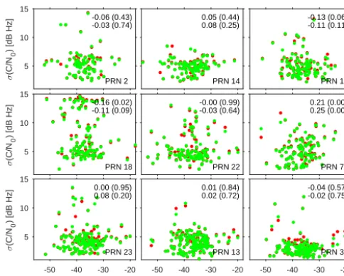
Figure 16. Same as Fig. 15 but the correlation analysis now in-cludes all observations at elevations between−2 and+2◦. With the exception of PRN 7 (and the Pearson’s coefficient for PRN 18) the derived correlations are no longer significant. Note the change of scale with respect to Fig. 15.
The MPS simulations (see Fig. 7) also suggest that the (negative) correlation betweenσ (C / N0)andhdN /dzi weakens if elevation angles close to or below the horizon are included. Figure 16 confirms this prediction. In contrast to Fig. 15 in this figure the elevation angle range, used for the calculation ofσ (C / N0), is extended downwards to−2◦. With the exception of both correlation coefficients for PRN 7 and the Pearson coefficient for PRN 18, the derived correla-tions are no longer significant; i.e. based on these results the null hypothesis cannot be rejected on the 5 % significance level.
An investigation of the relationship between signal am-plitude and frequency fluctuations, the local atmospheric re-fractivity field and, potentially, effects arising from surface topography is beyond the scope of this paper and will be ad-dressed with higher resolution meteorological data in future studies.
7 Conclusions
For more than a decade the OpenGPS receiver is used at GFZ in several ground-based and airborne measurement cam-paigns. Owing to its open hardware and software architecture the device can be adapted to address specific signal track-ing issues in GNSS radio occultation, reflectometry, scat-terometry or related fields. Here, a subset of low-elevation events recorded during the long-term GLESER campaign are introduced and discussed. Between 1 January and 31 De-cember 2014 the instrument recorded 2581 validated set-ting events at an observation site located at 52.3808◦N,
13.0642◦E. The OpenGPS receiver tracks signals from set-ting GPS satellites simultaneously in both, closed-loop and open-loop mode down to geometric elevation angles of−1 to
−1.5◦. These low-elevation events are characterized by fluc-tuations of about 10–20 dB Hz in signal-to-noise density ratio and about 10–20 Hz in carrier frequency. Tracking the same event with one closed-loop and two open-loop channels in parallel allows for direct intercomparison of open-loop ver-sus closed-loop performance. Whilst open-loop tracking al-lows us to follow strongly fluctuating signals to very low ele-vation angles, in about 14 % of the obserele-vations closed-loop tracking outperformed the open-loop channels, since fluctu-ations in the early phase of the setting event between+2 and 0◦elevation angle prevented proper initialization of the open-loop model.
The analysis of open-loop data is performed on demod-ulated in-phase and quad-phase correlation samples. The present study suggests that navigation message demodula-tion using external informademodula-tion, e.g. extracted from GFZ’s NavBit data base (doi:10.1594/GFZ.ISDC.GNSS/GNSS-GPS-1-NAVBIT), is preferable to internal demodulation. Open-loop signal tracking results are insensitive to the receiver-internal Doppler model for carrier signal-to-noise density ratios C / N0&30 dB Hz; below this value recon-structed Doppler frequencies gravitate towards the model value and thus potentially constitute a bias source. The present study did not address potential contributions of the ionospheric signal propagation and/or local multipath to the observed C / N0 fluctuations. These issues need to be ad-dressed in future work preferably using dual-frequency re-ceivers.
MPS simulations suggest that the observed weak to mod-erate correlations between mean vertical refractivity gradi-ents within the mean PBL and theC / N0fluctuations at posi-tive elevation angles are related to multipath induced by tilted layers of refractivity gradients. At lower elevation angles, be-low 0◦, signal diffraction at the ground surface dominates the observed amplitude variations.
8 Data availability
Appendix A
A1 OpenGPS receiver hardware
The OpenGPS instrument (a photograph of the PCI card is reproduced in Fig. A1) inherited its key design features from the OpenSourceGPS project (Kelley, 2002). It utilises the NovAtel® Superstar 1 (formerly CMC Electronics®) GPS module (outlined red in Fig. A1) and is based on the well-documented Zarlink® (formerly Mitel Semiconductor®) GPS chip set consisting of the single-frequency front-end GP2015 and the hardware correlator GP2021 (Zarlink, 2001).
During signal acquisition and tracking the 12 detection channels of the GP2021 hardware correlator provide in-phase and quad-in-phase correlation sums at the end of each full C/A code sequence. The occurrences are denoted DUMP events and repeat at a rate of about once every millisec-ond (Zarlink, 2001). DUMP events are aligned to the indi-vidual C/A code sequences and therefore are asynchronous events. A real-time operating system (Linux OpenSUSE ver-sion 11.3 with RTAI (RealTime Application Interface for Linux) version 3.8.1 kernel extension module) ensures that the correlator registers are read and processed within these time constraints.
In addition, the current values of the carrier and code NCOs are output as well. In contrast to DUMP events, these TIC events occur simultaneously on all active channels and can be triggered at a used-defined frequency. Linux RTAI meets the necessary time constraints for correlator input and output with latency times below about 3–5 µs as measured on the OpenGPS hardware.
The OpenGPS hardware utilises a modified Superstar 1 circuit board. Following the OpenSourceGPS concept (Kel-ley, 2002) the on-board processing unit ARM7TDMI and memory chip are unsoldered from the board and the mod-ified module is mounted on a PROTO-3 (manufactured by KOLTER ELECTRONIC®) prototyping board which plugs into a PCI expansion slot of a standard PC.
The signal acquisition and tracking program runs on the host computer; control, monitoring and readout of the GP2021 hardware correlator are performed through the PROTO-3’s PCI port. An interface module, which was de-signed and built in-house using discrete TTL logic (outlined blue in Fig. A1), connects to the hardware correlator’s input and output registers and allows direct access to the correlator registers from the host PC via the PCI interface bus.
Compared to conventional GPS receivers with on-board processing units, the OpenGPS design clearly has some dis-advantages. Using a PCI expansion card for signal front-end as well as down-conversion and performing signal acquisi-tion and tracking on a host PC implies larger size, mass and power consumption. However, the CPU processing power of the host PC surpasses the capabilities of the Superstar 1 onboard processor by a wide margin. The OpenGPS
instru-Figure A1.GFZ’s OpenGPS receiver board for PCI interface bus. A PCI prototyping board carries a modified single-frequency GPS module (red outline). Data cables connect the input/output ports of the hardware correlator chip to the TTL logic board (blue) and the PCI interface.
ment therefore allows us to operate the hardware correlator at higher sampling rates, to extract additional data from the correlation process (e.g. in-phase and quad-phase correlation samples from both GP2021 delay branches) and to run a full-featured operating system with network layer and graphical display capabilities in addition to the real-time process.
During the GLESER measurement campaign a mini-PC (Shuttle® XPC SB52G2) equipped with 760 MB memory and an Intel Pentium 4 processor clocked at 1.8 GHz serves as host PC. Despite this modest, by today’s standards, hard-ware the instrument supports sampling frequencies of up to 100 Hz; the observations described and discussed in this study are recorded at 50 Hz.
A2 OpenGPS receiver software
The OpenGPS signal acquisition, tracking and real-time pro-cessing software originates from the OpenSourceGPS project as well (Kelley, 2002); it also draws from source code written by S. Esterhuizen and S. van Leeuwen (van Leeuwen, 2002). The main tasks of the receiver program are
– search and acquisition in code and frequency space, – signal tracking using code delay and carrier
phase-locked loops,
– decoding of the navigation data modulation,
– calculation of transmitter position and velocity from broadcast ephemeris,
– calculation of receiver position and receiver clock bias from measured pseudoranges,
– output of raw data to disk.
Figure A2.Screenshot of a terminal window running the OpenGPS user space applicationogdspl. In the lower half characteristic infor-mation on the 12 tracking channels is shown. Note thatogdsplmaps azimuth angles to the interval[−180,+180◦]with−90 and+90◦ referring to west and east, respectively. At the time of the measurement on 16 October 2015 channel 1 tracked PRN 28 at an elevation angle of+1.64◦(column 6 entitled “elev”). Its azimuth value (−98.15◦) is within the selected observation window ([−160,−20◦]) and the O/L channels A and B, here listed as channel 11 and 12, are cloned from channel 1. In-phase and quad-phase samples as well as parameters describing the alignment between master and clone channels are listed at the very bottom of the screen. The top few lines list position and clock solutions from to the real-time navigation solution.
running in parallel, the kernel module ogrcvr_mod.ko and the user space application ogrcvr. The module ogrcvr_mod.koexecutes tasks controlling the code and carrier phase tracking loops. To maintain tracking lock the carrier phase and code data have to be read from the GP2021 registers, and the necessary loop adjustments have to be de-termined and written back to the correlator within a time in-terval of less than 100–200 µs. The real-time extension layer RTAI guarantees this latency performance even for high disk reading and writing operations or network traffic.ogrcvr handles deferrable tasks, such as determination of satellite positions and velocities from ephemeris data, calculation of the navigation solution and data storage. Communication be-tween real-time module and user space process is accom-plished using shared memory and FIFO (first in, first out) buffers. Inspection and modifications of relevant signal track-ing parameters, such as loop bandwidths and loop orders, O/L channel frequency and code offsets and sampling fre-quencies, are performed via aproc-based command line in-terface.
A third process,ogdspl, can optionally be started to dis-play tracking and positioning information on the terminal screen (Fig. A2). In total, the source code of all kernel and user space modules comprises about 20 000 lines of C code. The OpenGPS receiver operates in two different observa-tion modes. In “monitor mode” up to 10 of the 12 correlator channels are assigned to PRNs of visible GPS satellites. The O/L channels A and B, in Fig. A2 listed as number 11 and
12, remain unassigned. When a satellite, tracked by channel numberk, crosses the+2◦elevation boundary from above, the receiver transitions to “measurement mode”, channels A and B are assigned to this satellite’s PRN and their code and carrier NCOs are aligned to those of channelkas well. In the following this process is called “cloning” of A and B from the “master” channelk and A/B are referred to as “clone” channels.
In measurement mode code and carrier NCO data, in-phase and quad-in-phase correlation sums from both GP2021 correlation branches (“prompt” and “dither”) and position and clock bias results from the real-time navigation solu-tion are stored on the local hard disk. The delay between the prompt and dither branch is fixed at 0.5 chips (about 150 m). Code, carrier phases and correlation sums are written with a temporal resolution of Ts=0.02 ms (corresponding to a sampling frequency offs=50 Hz); the navigation solution is provided once per second. We note that the stored corre-lation sums are coherently integrated over Ts, whereas the NCO code and carrier phase are instantaneous values sam-pled at the corresponding TIC event.
Typically, measurement mode lasts for about 10–15 min and ends when the satellite’s elevation angle drops below
−2◦. During an initialization phase, for elevation angles above 0◦, the code and carrier phase loop adjustments are collected at each TIC event and stored. Thereafter, when el-evation angles are below 0◦, the carrier loop is opened and
the stored Doppler adjustments. For code O/L tracking a hybrid method is employed; ifC / N0≤30 dB Hz, the code NCO values are calculated from a second-order polynomial extrapolation of the stored adjustments. Otherwise, the code loop operates in C/L mode; in addition, the difference be-tween actual adjustments and model-derived values is saved and added to the model. Thus, potential deviations between observations atC / N0>30 dB Hz and the extrapolated loop adjustments are used to update the model.
The OpenGPS receiver software determines geometric el-evation angles from GPS almanac information. Since the data post-processing analysis is based on the more precise GPS ephemeris data, the elevation angles of the measurement start and the end of the O/L initialization may deviate from the nominal values of+2 and 0◦, respectively, by some tenths of a degree (see e.g. insert in Fig. 3).
Closer inspection of the O/L carrier NCO frequencies in Fig. 3 (red and green lines; the insert shows a zoomed-in view) reveals residual deviation of the O/L channel from the target Doppler model in addition to the nominal val-ues of ±5 Hz. First, at the start of O/L tracking mode (at about −0.08◦ elevation angle) the two clone channels are gradually moved into phase alignment to the O/L model by adjusting the corresponding NCO frequencies (OpenGPS’s hardware correlator GP2021 does not support carrier phase adjustments). For channel B (+5 Hz) the duration of this initialization process is shorter, since its initial phase hap-pened to be closer to the model phase. Furthermore, even af-ter completion of the alignment process, small fluctuations on the order of a few 100 mHz are still apparent. These fluctuations are caused by the finite bandwidth of a dedi-cated feedback loop, which keeps the two O/L channels sep-arated by 10 Hz in Doppler space. (Accessing the GP2021’s MULTI_CHANNEL_SELECT registers led to adverse side effects in our tests.)
Acknowledgements. Helpful discussions with Stefan Heise are gratefully acknowledged. Thoughtful comments and valuable suggestions from two anonymous reviewers significantly improved this paper. We thank Christian Selke and Martin König for the design and assembly of the OpenGPS hardware and Potsdam Institute for Climate Impact Research for access to the observation deck on building A31. GPS broadcast ephemeris data were provided by GFZ’s orbit processing group at Oberpfaffenhofen, Germany. The OpenGPS receiver software is derived from the GPL-licensed OpenSourceGPS code base written by Clifford Kel-ley with contributions from Stephan Esterhuizen and Sam Storm van Leeuwen. The European Centre for Medium-Range Weather Forecasts (ECMWF) is acknowledged for access to meteorological analysis data. Trademarks are owned by their respective owners.
The article processing charges for this open-access publication were covered by a Research
Centre of the Helmholtz Association.
Edited by: J. Joiner
Reviewed by: two anonymous referees
References
Anderson, K. D.: Determination of water level and tides us-ing interferometric observations of GPS signals, J. At-mos. Ocean. Tech., 17, 1118–1127, doi:10.1175/1520-0426(2000)017<1118:DOWLAT>2.0.CO;2, 2000.
Anthes, R. A., Bernhardt, P. A., Chen, Y., Cucurull, L., Dymond, K. F., Ector, D., Healy, S. B., Ho, S.-P., Hunt, D. C., Kuo, Y.-H., Liu, Y.-H., Manning, K., McCormick, C., Meehan, T. K., Ran-del, W. J., Rocken, C., Schreiner, W. S., Sokolovskiy, S. V., Syndergaard, S., Thompson, D. C., Trenberth, K. E., Wee, T.-K., Yen, N. L., and Zeng, Z.: The COSMIC/FORMOSAT-3 mission: Early results, B. Am. Meteor. Soc., 89, COSMIC/FORMOSAT-31COSMIC/FORMOSAT-3–COSMIC/FORMOSAT-3COSMIC/FORMOSAT-3COSMIC/FORMOSAT-3, doi:10.1175/BAMS-89-3-313, 2008.
Ao, C. O., Meehan, T. K., Hajj, G. A., Mannucci, A. J., and Beyerle, G.: Lower-troposphere refractivity bias in GPS occultation retrievals, J. Geophys. Res., 108, 4577, doi:10.1029/2002JD003216, 2003.
Ao, C. O., Hajj, G. A., Meehan, T. K., Dong, D., Iijima, B. A., Mannucci, A. J., and Kursinski, E. R.: Rising and setting GPS occultations by use of open-loop tracking, J. Geophys. Res., 114, D04101, doi:10.1029/2008JD010483, 2009.
Axelrad, P., Larson, K., and Jones, B.: Use of the correct satellite repeat period to characterize and reduce site-specific multipath errors, in: Proceedings of the 18th International Technical Meet-ing of the Satellite Division of The Institute of Navigation (ION GNSS 2005), 2638–2648, IEEE, Long Beach, CA, 2005. Badke, B.: What isC / N0and how is it calculated in a GNSS
re-ceiver?, InsideGNSS, 4, 20–23, 2009.
Bevis, M., Businger, S., Chiswell, S., Herring, T. A., An-thes, R. A., Rocken, C., and Ware, R. H.: GPS meteo-rology: Mapping zenith wet delays onto precipitable wa-ter, J. Appl. Meteorol., 33, 379–386, doi:10.1175/1520-0450(1994)033<0379:GMMZWD>2.0.CO;2, 1994.
Beyerle, G., Gorbunov, M. E., and Ao, C. O.: Simulation studies of GPS radio occultation measurements, Radio Sci., 38, 1084, doi:10.1029/2002RS002800, 2003.
Beyerle, G., Wickert, J., Schmidt, T., and Reigber, C.: GPS ra-dio occultation with GRACE: Atmospheric profiling utilizing the zero difference technique, Geophys. Res. Lett., 32, L13806, doi:10.1029/2005GL023109, 2005.
Beyerle, G., Ramatschi, M., Galas, R., Schmidt, T., Wickert, J., and Rothacher, M.: A data archive of GPS navigation messages, GPS Solut., 13, 35–41, doi:10.1007/s10291-008-0095-y, 2009. Beyerle, G., Grunwaldt, L., Heise, S., Köhler, W., König, R.,
Micha-lak, G., Rothacher, M., Schmidt, T., Wickert, J., Tapley, B. D., and Giesinger, B.: First results from the GPS atmosphere sound-ing experiment TOR aboard the TerraSAR-X satellite, Atmos. Chem. Phys., 11, 6687–6699, doi:10.5194/acp-11-6687-2011, 2011.
Bonnedal, M., Christensen, J., Carlström, A., and Berg, A.: Metop-GRAS in-orbit instrument performance, GPS Solut., 14, 109– 120, doi:10.1007/s10291-009-0142-3, 2010.
Braun, J., Rocken, C., and Ware, R.: Validation of line-of-sight water vapor measurements with GPS, Radio Sci., 36, 459–472, doi:10.1029/2000RS002353, 2001.
Businger, S., Chiswell, S. R., Bevis, M., Duan, J. P., Anthes, R. A., Rocken, C., Ware, R. H., Exner, M., VanHove, T., and Solheim, F. S.: The promise of GPS in atmospheric mon-itoring, B. Am. Meteor. Soc., 77, 5–18, doi:10.1175/1520-0477(1996)077<0005:TPOGIA>2.0.CO;2, 1996.
Choi, K., Bilich, A., Larson, K. M., and Axelrad, P.: Modified side-real filtering: Implications for high-rate GPS positioning, Geo-phys. Res. Lett., 31, L22608, doi:10.1029/2004GL021621, 2004. Cucurull, L., Derber, J. C., Treadon, R., and Purser, R. J.: Assim-ilation of Global Positioning System radio occultation observa-tions into NCEP’s global data assimilation system, Mon. Weather Rev., 135, 3174–3193, doi:10.1175/MWR3461.1, 2007. Dick, G., Gendt, G., and Reigber, C.: First experience with near
real-time water vapor estimation in a German GPS network, J. Atmos. Sol.-Terr. Phy., 63, 1295–1304, doi:10.1016/S1364-6826(00)00248-0, 2001.
Elósegui, P., Davis, J. L., Jaldehag, R. T. K., Johansson, J. M., Niell, A. E., and Shapiro, I. I.: Geodesy using the Global Po-sitioning System: The effects of signal scattering on estimates of site position, J. Geophys. Res.-Sol. Ea., 100, 9921–9934, doi:10.1029/95JB00868, 1995.
Emardson, T. R., Elgered, G., and Johansson, J. M.: Three months of continuous monitoring of atmospheric water vapor with a net-work of Global Positioning System receivers, J. Geophys. Res.-Atmos., 103, 1807–1820, doi:10.1029/97JD03015, 1998. Foelsche, U., Scherllin-Pirscher, B., Ladstädter, F., Steiner,
A. K., and Kirchengast, G.: Refractivity and temperature cli-mate records from multiple radio occultation satellites con-sistent within 0.05 %, Atmos. Meas. Tech., 4, 2007–2018, doi:10.5194/amt-4-2007-2011, 2011.
Gaylor, D. E., Lightsey, E. G., and Key, K. W.: Effects of mul-tipath and signal blockage on GPS navigation in the vicinity of the International Space Station (ISS), Navigation, 52, 61–70, doi:10.1002/j.2161-4296.2005.tb01732.x, 2005.