Interannual evolution of (sub)mesoscale dynamics in the Bay of Biscay

(1)

Ocean Sci., 13, 777–797, 2017

https://doi.org/10.5194/os-13-777-2017

Interannual evolution of (sub)mesoscale dynamics

in the Bay of Biscay

Guillaume Charria1, Sébastien Theetten1, Frédéric Vandermeirsch1, Özge Yelekçi1, and Nicole Audiffren2

1_{Ifremer, Univ. Brest, CNRS, IRD, Laboratoire d’Océanographie Physique et Spatiale (LOPS), IUEM, 29280 Brest, France} 2_{CINES, 34090 Montpellier, France}

Correspondence to:Guillaume Charria ([email protected]) Received: 29 November 2016 – Discussion started: 26 January 2017

Revised: 6 August 2017 – Accepted: 8 August 2017 – Published: 25 September 2017

Abstract.In the north-east Atlantic Ocean, the Bay of Bis-cay is an intersection between a coastal constrained dynam-ics (wide continental shelf and shelf break regions) and an eastern boundary circulation system. In this framework, the eddy kinetic energy is 1 order of magnitude lower than in western boundary systems. To explore this coastal complex system, a high-resolution (1 km, 100 vertical sigma layers) model experiment including tidal dynamics over a period of 10 years (2001–2010) has been implemented. The ability of the numerical environment to reproduce main patterns over interannual scales is demonstrated. Based on this experiment, the features of the (sub)mesoscale processes are described in the deep part of the region (i.e. abyssal plain and continental slope). A system with the development of mixed layer insta-bilities at the end of winter is highlighted. Beyond confirm-ing an observed behaviour of seasonal (sub)mesoscale activ-ity in other regions, the simulated period allows exploring the interannual variability of these structures. A relationship between the winter maximum of mixed layer depth and the intensity of (sub)mesoscale related activity (vertical velocity, relative vorticity) is revealed and can be explained by large-scale atmospheric forcings (e.g. the cold winter in 2005). The first submesoscale-permitting exploration of this 3-D coastal system shows the importance of (sub)mesoscale activity in this region with its evolution implying a potentially signifi-cant impact on vertical and horizontal mixing.

1 Introduction

(2)

778 G. Charria et al.: Interannual evolution of (sub)mesoscale dynamics in the Bay of Biscay

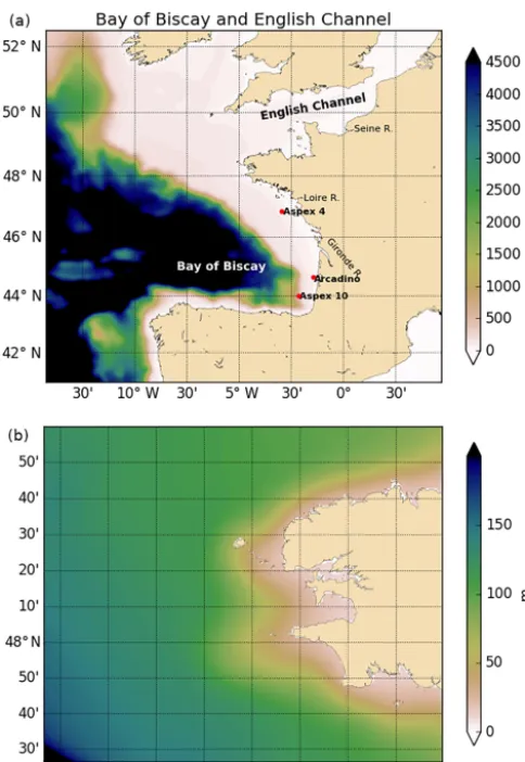
Figure 1.Bathymetry of the modelled region(a). Red points corre-spond to the mooring sites used for model validation. A zoomed-in area around 48◦N is represented in panel(b).

Molemaker et al., 2015). This dynamics is particularly active (in terms of eddy kinetic energy) in western boundary cur-rents.

In the present study, we aim at contributing to the descrip-tion and the understanding of small-scale features in east-ern boundary regions where the average level of kinetic en-ergy remains low (Caballero et al., 2008; Dussurget et al., 2011) and of the mesoscale and submesoscale activity impact on long-term fluctuations related to evolution in atmospheric conditions.

The considered definition for the studied scales, depending on the depth of the water column and the stratification, has to be recalled as we progress in a coastal environment. In this framework, the mesoscale is defined by scales around the in-ternal Rossby radius of deformation (∼20–50 km in the mid-latitudes; Chelton et al., 1998) where the flow is adjusted un-der the effect of the rotation. Over the continental shelf, this internal Rossby radius of deformation decreases to values around 3–8 km (M. Valdivieso Da Costa et al., personal com-munication, 2006), for example, in the Bay of Biscay. The

submesoscale, as introduced by McWilliams (1985), refers to scales lower than the internal Rossby radius of deformation where the influence of the Earth’s rotation tends to decrease in order to reach a non-rotating regime of three-dimensional turbulence (Kolmogorov, 1941). Submesoscale is then rang-ing from O(100) m to O(10) km over the continental shelf and in the open ocean (Capet et al., 2008b; Thomas et al., 2008). In the present work, we refer to (sub)mesoscale (i.e. mesoscale and submesoscale features) for processes with a length scale lower than 40 km.

In the Bay of Biscay abyssal plain, coherent mesoscale structures have been identified like the long-lived anticy-clonic Slope Water Oceanic eDDIES (SWODDIES) de-scribed by Pingree and Le Cann (1992a, b) generated by slope current instabilities or quasi-stationary eddies in the south-eastern Bay of Biscay (Caballero et al., 2013, 2016). Following satellite altimetry-based studies in the region (Ca-ballero et al., 2008; Dussurget et al., 2011), observations of mesoscale variability have been described with higher eddy kinetic energy from December to May. However, the spa-tiotemporal resolution and coverage from altimetry does not allow exploring underlying processes and interannual vari-ability at submesoscale.

In this context, after controlling the efficiency and accu-racy of a coastal model with a 1 km spatial resolution to reproduce the observed processes in the Bay of Biscay, the (sub)mesoscale variability at annual and interannual scales is explored as a first step to define the role of related vertical motions at small scales on long-term evolution and associ-ated biogeochemical production.

2 Numerical framework 2.1 Model description

Numerical simulations are based on the MARS3D model1. MARS3D (Duhaut et al., 2008; Lazure and Dumas, 2008) is a primitive equation model with a free surface to rep-resent the gravity waves in the coastal area. In this finite-difference code, the primitive equations are discretized on an Arakawa C-grid centred at tracer points (Mesinger and Arakawa, 1976). The sigma coordinates are used on the ver-tical dimension to resolve simultaneously the shallow and deep waters. A specificity of MARS3D model is that the barotropic mode and baroclinic mode are using the same time step and the barotropic mode is resolved by an alternating di-rection implicit method (Lazure and Dumas, 2008). Detailed equations are given in Appendix A.

The new numerical MARS code can run without explicit viscosity (Duhaut et al., 2008). The k- turbulent closure scheme is used to model vertical mixing (Rodi, 1993).

(3)

G. Charria et al.: Interannual evolution of (sub)mesoscale dynamics in the Bay of Biscay 779 2.2 Numerical experiments

The MARS3D model has already been used to investigate the Bay of Biscay and its extension to the western English Channel and focused on the validation of hydrology on the French continental shelf with a 4 km horizontal resolution and 30 vertical levels (Lazure et al., 2009). In this new con-figuration (Theetten et al., 2017), the model domain extends from the Bay of Biscay to the English Channel from 41 to 52.5◦N and 14.3◦W to 4.5◦E, with a 1 km spatial horizon-tal resolution with a time step of1t=60 s. This configura-tion (called BACH1000_100lev) has 1449×1282 grid points and uses 100 vertical sigma levels. The vertical discretization is a generalized vertical, terrain-following coordinate system (withhc=20 m;θ=6 andb=0;hcis the shallower depth above which we wish to have more resolution,θ andb are surface and bottom control parameters; Appendix A). The bathymetry is a composite of several IFREMER digital ter-rain models (DTMs) with 100 m resolution along the coast covering the French part of continental shelf completed by a 1 km resolution DTM covering the bay of Biscay and fi-nally completed by a 1 nautical mile resolution from the North West Shelf Operational Oceanographic System (http: //noos.bsh.de). Both digital terrain models and mean sea level are interpolated on the grid and merged (Fig. 1). Some hand editing has been performed in few key areas specially to cor-rect spurious interpolation near the coastline. The maximum depth in the model is 5310 m. The interpolated topographies are smoothed by selectively applying a local filter to reduce therfactor to below 0.25 (r=1h/2h, wherehis the depth of the water column; Haidvogel and Beckmann, 1999). River runoffs are provided from 95 chronological records (daily measurements and climatology for the past years when no observations are available) located on the Spanish, French, Dutch, British and Irish coasts.

Initial conditions for temperature, salinity, sea surface height, baroclinic and barotropic velocities (calculated from baroclinic components) are derived from a DRAKKAR global configuration named ORCA12_L46-MJM88 (Mo-lines et al., 2014). At the open ocean boundaries, the same variables as initial conditions are used with adaptive bound-ary conditions in a sponge layer on the north, south and west boundaries (Marchesiello et al., 2001). The sponge layer width is 20 km and the maximum horizontal viscos-ity/diffusivity values are 100 m2s−1and 0 outside the open boundary layers. The tide with 14 harmonic constituents is imposed along the boundaries using the FES2004 ocean tide atlas (Lyard et al., 2006).

The atmospheric forcing, which drives the simulation presented here, is provided by ERA-Interim, produced by the European Centre for Medium-Range Weather Forecasts (ECMWF; Berrisford et al., 2011). Using the 2 m air tem-perature, atmospherical pressure, relative humidity, rain and cloud cover from ERA-Interim data, indirect calculation of the different components of the air–sea heat exchange are

computed by several bulk formulae (from Lazure et al., 2009).

The simulation starts from 1 January 2001 and covers a 10-year period until 31 December 2010. A spin-up of 2 years is taken into account to set up an established sea-sonal cycle in the circulation even in the open ocean con-strained by a large-scale solution forced in open bound-ary conditions. The analysed period is then run from 2003 to 2010. The BACH1000_100lev configuration is imple-mented on the Tier-1 supercomputer machine OCCIGEN provided by GENCI and hosted at CINES2. The supercom-puter OCCIGEN with a performance peak of 2.1 Pflops en-compasses 2106 dual-socket nodes on an Intel Xeon Haswell cadenced at 2.6 GHz. A total of 12 cores are present on each socket. This numerical experiment was part of the “Big Challenges program” conducted during the VRS period from December 2014 to January 2015. Using a domain decom-position technique, the computational domain is split into 558 subdomains leading to the same number of MPI tasks with 12 OpenMP threads each. This hybrid MPI/OpenMP application runs on 6696 cores and produces daily averaged outputs using the input/output server XIOS3specially imple-mented in MARS3D for this configuration.

3 Bay of Biscay features from a spatial high-resolution simulation

Before exploring (sub)mesoscale features in the Bay of Bis-cay, the ability of the numerical experiment to reproduce known processes in the region needs to be evaluated. Fol-lowing a general view of the modelled fields, a few key diag-nostics on the hydrology and the circulation are presented. 3.1 Sea surface temperature and salinity

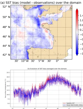
The numerical experiment is validated using remotely sensed sea surface temperature (SST). Based on SEVIRI SST re-motely sensed data (METEOSAT SST provided by OSI-SAF belonging to EUMETSAT with ∼2 km spatial resolution), modelled fields are evaluated. In Fig. 2a, the mean bias be-tween observed and modelled SST over 2010 is computed:

hSSTbiasilong,lat,t=  

1

(NiNjNt)

Ni,Nj,Nt

X i=1,j=1,t=1

SSTmodel_i,j,t   −   1

(NiNjNt)

Ni,Nj,Nt

X i=1,j=1,t=1

SSTobservations_i,j,t  ,

whereNiNjNt is the number of grid points in space and time.

2_{http://www.cines.fr,} _Centre _Informatique _National _de l’Enseignement Supérieur (CINES)

(4)

Figure 2.Comparison between observed (SEVIRI satellite SST) and modelled (BACH1000_100lev simulation) sea surface temperature (SST).(a)Mean bias between model and observations for the year 2010.(b)Temporal evolution of the spatial mean SST bias during 2010. The shading around the curves represents the spatial standard deviation (i.e. the standard deviation over the domain computed for each time step).

At the end of the experiment, this bias shows an av-eraged underestimation of the temperature by the model (−0.24±0.28◦C over the domain). These biases do not ex-ceed 1.75◦C. Such large values are obtained in two regions. First, in the Ushant front region (around 47.5–49◦N and 5– 6◦W; Le Boyer et al., 2009), the model underestimates the SST. This bias can be explained by the variability of the Ushant front, developed during stratified seasons, which re-mains complex to reproduce (Renaudie et al., 2011; Pasquet et al., 2012). The second main bias exceeding 1.5◦C is lo-cated along the western Spanish coast. The shape of the bias is typical of upwelling extent in this region. In this case, the coarse atmospheric forcing resolution can be emphasized as the major error source. Figure 2b shows the temporal

varia-tion of the spatial averaged bias:

hSSTi_long_,_lat_{(t )}= 1

(NiNj) Ni,Nj

X i=1,j=1

SSTi,j,t,

whereNiNj is the number of grid points in space. The shad-ing around the curves represents the spatial standard devia-tion:

σSST(t )= v u u t

1

(Ni−1)(Nj−1) Ni,Nj

X

i=1,j=1

(SSTi,j−<SST>lon,lat(t ))2.

(5)

G. Charria et al.: Interannual evolution of (sub)mesoscale dynamics in the Bay of Biscay 781

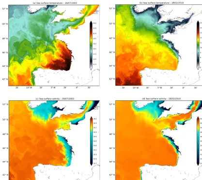
Figure 3.Example of modelled (BACH1000_100lev configuration) sea surface temperature(a, b)and salinity(c, d)in summer (a, c– 28 July 2003) and winter (b, d– 27 February 2010).

(6)

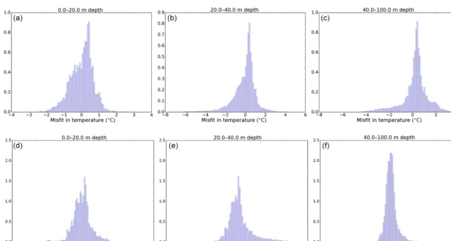
Figure 5.Normalized distribution of the misfit (modelled–observed) in temperature(a, b, c)and salinity(d, e, f)from RECOPESCA and Argo in situ profiles (only for profiles deeper than 100 m) for three vertical layers: 0–20 m depth(a, d), 20–40 m depth(b, e)and 40–100 m depth(c, f). The integral of the histogram sums up to 1.

developed seasonal cycle with maximum temperature in Au-gust and September and the coldest waters at the end of win-ter in March. The largest differences can be noticed during the onset of the seasonal stratification in May–June.

After this first overview on SST, two contrasted dates (summer and winter) are displayed in Fig. 3 for SST and sea surface salinity (SSS). In summer (Fig. 3a), the model re-produces the warm pool in the south-eastern part of the Bay of Biscay with temperature exceeding 21◦C (Lazure et al., 2009). In front of Brittany (48.2◦N, 5.6◦W), the position of the Ushant tidal front (Le Boyer et al., 2009; Renaudie et al., 2011; Pasquet et al., 2012) with cold waters in the vicinity of the coast and warmer water outside the front is reproduced by model simulations. In winter, colder (Fig. 3b) and fresher (Fig. 3d) waters above the inner shelf related to river plume extent do not exceed 9◦_{C and salinity of 34.8.}

Furthermore, in Fig. 3, turbulent activity (eddies, fila-ments) can be noticed during summer and winter in the deeper region but also over the continental shelf.

As a more focused illustration, freshwater exports in the open ocean, as described in Reverdin et al. (2013), appear in the present experiment (Fig. 4). The elongated freshwater fil-aments extending to the south-west in the southern part of the Bay of Biscay (44◦N, 3.5◦W) represent an observed signal of cross-slope exchanges. Reproducing these exports is a sig-nificant step forward in our simulations, thanks to the higher spatial resolution (1 km vs. 4 km in previous experiments). Indeed, the spatial resolution appeared as a key issue to

bet-ter resolve these exchanges between the continental shelf and the open ocean.

3.2 Vertical hydrological structure

The hydrological content of the simulation is evaluated through comparisons with available observations in 2010 from the CORA-IBI (COriolis ocean database for ReAnal-ysis – Ireland–Biscay–Iberia, Szekely et al., 2017) database. Considered vertical profiles can be divided into two sources: Argo (Argo, 2000; Riser et al., 2016) profiles in the open ocean and RECOPESCA (Leblond et al., 2010; Charria et al., 2014; Lamouroux et al., 2016) profiles on the continental shelf.

Figure 5 shows the difference between observed and mod-elled profiles for the year 2010 in temperature and salinity in the top layers. In temperature, the model reproduces the vertical structure with a small average misfit of 0.015 and a 0.45◦C root mean square error (RMSE) between 0 and 20 m depth (Fig. 5a),−0.11◦C (1.23◦C for RMSE) between 20 and 40 m depth (Fig. 5b) and 0.25◦_{C (1.17}◦_{C RMSE)}

(7)

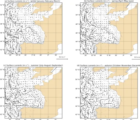
Figure 6.Average modelled seasonal circulation (a: winter,b: spring,c: summer,d: autumn) for surface layers (0–50 m depth) over the period 2001–2010 (for clarity purposes, fields have undersampled and 1 over 50 grid points are plotted). Gray lines represent 500, 200, 100 and 50 m isobaths.

layer 0–20 m depth, RMSE=0.27; Fig. 5d) and above 100 m depth (0.025 for the layer 40–100 m depth, RMSE=0.28; Fig. 5e and f) than between 20 and 40 m depth where the average difference is larger (0.176, RMSE=0.59). Consid-ering the RMSE, we confirm that the maximum of error is located in mid-depth layers (20–40 m) and can be locally im-portant. Part of the error can be attributed to the colocation approach assuming that we will reproduce the same features at the same time and place in the simulations, but choices for the configuration (e.g. smoothed bathymetry, coarse atmo-spheric forcings) can contribute to increasing the observed error between model and local in situ observations. However, following the distributions, with biases of different signs fol-lowing the depth, no systematic bias exists in the numerical experiment.

3.3 Bay of Biscay general circulation

Concerning the general circulation in the region, three levels of comparisons are detailed. As a synoptic view, the seasonal circulation in the surface layer is computed to be compared with existing climatologies (e.g. Charria et al., 2013). Then, to highlight circulation patterns occurring at short timescales as poleward jets over the continental shelf (e.g. Batifoulier et al., 2012; Kersalé et al., 2015) and the vertical structure of the currents, modelled fields are compared with ADCP observations during the ASPEX campaign (Le Boyer et al., 2013; Kersalé et al., 2015) and the front of the Arcachon Bay during the ARCADINO campaign (Batifoulier et al., 2012).

(8)

cli-784 G. Charria et al.: Interannual evolution of (sub)mesoscale dynamics in the Bay of Biscay

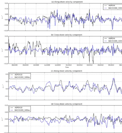
Figure 7.Comparison of the 1-day mean and depth averaged along-shore and cross-shore velocity components between ADCP measurements (black) and BACH1000_100lev currents (blue) at the location of ASPEX4 (Fig. 7a and b) above the continental shelf and ASPEX10 (Fig. 7c and d) above the continental slope. The orientation of the along-shore and cross-shore components is relative to the bathymetry.

matology (processed from observation from 1992 to 2009) derived from drifters in Charria et al. (2013). In winter (Fig. 6a), the contrasted velocities with weak current over the continental shelf and more intense structures in the open ocean clearly appear. The poleward slope current with val-ues lower than 10 cm s−1is reproduced. In spring (Fig. 6b), the reversal of circulation with an equatorward slope current is simulated. This circulation remains sustained in summer (Fig. 6c) with a reinforcement of equatorward currents over the continental shelf. Following wind regime evolution and the transition period in September–October (SOMA seasonal response; Pingree et al., 1999), autumn circulation (Fig. 6d) highlights, on average, the poleward slope current close to

the 500 m isobath. These average circulation features are then in agreement with the drifter-derived seasonal climatology (Charria et al., 2013).

Another source for validating the modelled circulation comes from ADCP deployments in the region. During the ASPEX project, 10 current-meter moorings were deployed from July 2009 to August 2011. The mooring location was distributed over the continental shelf and the upper section of the shelf break. Mooring features and observations from the project are described and analysed in Le Boyer et al. (2013) and Kersalé et al. (2015).

(9)

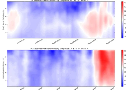
Figure 8.Evolution of meridional velocity component in m s−1of the BACH1000_100lev model during July–August 2008(a)at the AR-CADINO ADCP location. ADCP observations for the same periods are represented(b).

4 on the continental shelf and no. 10 on the continental slope (see positions in Fig. 1). We can notice that the length of the considered time series for comparison is both limited by the duration of the numerical experiment (2001–2010) and the technical issues in data sampling (lack of measurements for the end of the ASPEX10 time series). Two-dimensional linear spatial interpolation on model output velocity compo-nents at each sigma level is made on the geographical posi-tion/location of the mooring. Then, the zonal and meridional components of modelled velocities are projected on along-shore and cross-along-shore component at each sigma level. In the aim to compare the depth-averaged velocity on both model outputs and in situ data, vertical integration of the two veloc-ity components is made on almost the whole water column4. Vertical integration of the model outputs is also made on the water column between the minimum and maximum depths defined previously.

In Fig. 7, the modelled and observed currents are repre-sented. A general agreement following the current directions and amplitudes is observed with correlations between 0.6

4_{The first record is located near the bottom. Records located in} the surface layer thickness (corresponding to 20 % of the mooring depth) have been removed due to noisy measurements.

and 0.69 for along-shore components. For the cross-shore component, representing the less intense currents, in AS-PEX4 (Fig. 4b), the direction of the current is well repro-duced but the amplitude remains generally smaller in simu-lations (RMSE=0.024 m s−1₎_{. At ASPEX10 (Fig. 4d), the} cross-shore weak circulation is not reproduced, with a corre-lation between model and observation equal to 0.09, due to the mesoscale circulation in this area (e.g. Solabarrieta et al., 2014; Caballero et al., 2016). The agreement between obser-vations and numerical simulation is improved for dominant along-shore currents. Indeed, amplitudes are very similar in both ASPEX sites (except during autumn 2009; Fig. 4a and c). The direction and direction changes are also very well re-produced (the correlation for ASPEX4 is equal to 0.6 and for ASPEX10 to 0.69), even at high frequency, which was not expected following the coarse atmospheric forcings used for the simulation.

Other comparisons have been performed with an ADCP mooring during the ARCADINO experiment. This mooring, located on the Aquitaine shelf (south of 45◦_{N; Fig. 1), has}

(10)

Au-786 G. Charria et al.: Interannual evolution of (sub)mesoscale dynamics in the Bay of Biscay

Figure 9.Surface modelled relative vorticity for 28 July 2003(a)and 27 February 2010(b). The yellow rectangle limits the targeted region for diagnostics.

gust 2008 (Fig. 8) in observations. From in situ ADCP mea-surements (Batifoulier et al., 2012), there is also a velocity maximum between 16 and 20 August 2008. In the mod-elled fields, the jet is reproduced but velocities are weaker and the event starts earlier in the simulation. The jet is also deeper in the model (20–40 m depth with maximum veloc-ities ∼16 cm s−1₎ _{than in observations with a maximum} above 30 m depth. When model forcings are explored, we ex-plain this event with similar conditions to those observed in Batifoulier et al. (2012). Indeed, westerly winds are blowing from the 6 to 8 August (with intensities 8 to 12 m s−1)along the Spanish coast to set up the circulation resulting in the poleward jet following the explained process in Batifoulier et al. (2012).

These illustrations of the modelled fields and comparisons with available observations show the ability and the limits of our numerical experiment to reproduce the coastal ocean dynamics at high resolution in the Bay of Biscay. Based on these fields, the interannual variability at (sub)mesoscales can be explored.

4 Interannual variability of (sub)mesoscale instabilities in surface layers

The present study aims to characterize the interannual vari-ability of the (sub)mesoscale dynamics and discuss the possi-ble processes explaining this variability. Before considering these interannual scales, the seasonal features are described for a given year.

4.1 Seasonal scale

To explore the (sub)mesoscale activity, the vertical compo-nent of the relative vorticity (referred as relative vorticity) has been first analysed. From these dynamical fields, we can infer the intensity of rotating structures and their spatial dis-tribution.

In Fig. 9, the surface relative vorticity from analysed simu-lations at different contrasted time steps is represented. From these maps, different patterns can be noticed. First, the con-trast between the deep open ocean and the shallow continen-tal shelf is clearly visible for the different periods. In sum-mer 2003 (Fig. 9a), over the continental shelf, the internal waves are observed in the northern part of the domain spread-ing from the shelf break (around 47.5–48◦N, 7–5◦W). In the southern part of the continental shelf (south of 48◦N), small structures related to local drivers (e.g. edge of region of freshwater influence, wind bursts; O. Yelekci et al., per-sonal communication, 2016) are developed. These structures can be seen through large relative vorticity values over the outer part of the continental shelf between the 100 m isobath (Fig. 6) and the shelf break (Fig. 1). In contrast, in winter (Fig. 9b), small-scale features are more concentrated in the inner shelf (the first half of the continental shelf closer to the coast with water shallower than 100 m depth) under the influ-ence of large winter river inputs (e.g. mainly from the Loire and Gironde rivers).

(11)

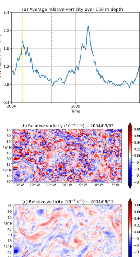
Figure 10.Relative vorticity averaged over 150 m depth and spa-tially averaged for the years 2004 and 2005(a). Map of the surface relative vorticity for 2 March 2004(b)and 15 August 2004(c).

are larger than in winter. More large-scale vortices are simu-lated during this season. The spatial spectral analysis over the domain (Fig. 11) confirms the largest small-scale (< 50 km wavelength) variance peaks in winter (maximum in March) and the minimum variance at small scale in summer (July).

Based on Fig. 10, representing the years 2004 and 2005, a picture of the annual evolution of the relative vorticity in-tensity can be drawn considering a spatial average of the ab-solute relative vorticity over the region highlighted in Fig. 9 (yellow rectangle). Based on the spatial average integrated over 150 m depth5 (Fig. 10a), a maximum is observed dur-5_{This depth (150 m) has been defined to include most of the} mixed layer depth in winter. As it is used for the whole time

se-Figure 11.Power spectrum (computed for each latitude and aver-aged over longitudes and time during the considered month) from surface relative vorticity for the year 2010(a). Numbers in the leg-end correspond to the months in the year 2010. Time series of the regressed spectral slope from the power spectrum of surface relative vorticity in 2010(b). Spectral slopes have been computed consider-ing wavelengths from 7 to 132 km.

(12)

Figure 12.Vertical velocity averaged over 150 m depth and spa-tially averaged for the years 2004 and 2005(a). Map of the vertical velocity at 4 m depth for 2 March 2004(b)and 15 August 2004(c).

month. These spectra clearly show the seasonal variation of the variance with a maximum in March and a minimum in July. An increase in the variance of small scales (lower than 50 km) is also observed through a change in the curve slope observed in November, January and March compared with May, July and September.

Following the relative vorticity fields (i.e. related to vor-tices, fronts, filaments), vertical motions can also be ex-plored. The role of structures at (sub)mesoscale on these ver-tical motions can be highlighted by the exploration of verver-tical velocities (significant vertical velocity patterns are mainly at submesoscales and mesoscales). Indeed, in Fig. 12a, a sim-ilar seasonal cycle with relative vorticity is observed with a maximum of integrated vertical velocity at the end of win-ter (February–March) and a minimum in summer (June– September). Based on the spatial patterns of the vertical

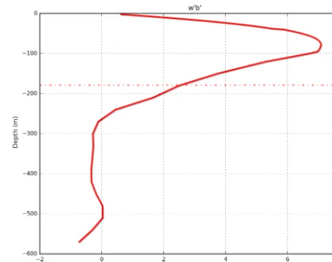
ve-Figure 13.Vertical profile ofw0b0 averaged over the studied sub-domain (described in Fig. 9) during the winter season (January– February–March) in 2005. The dashed line represents the mixed layer depth averaged for the same period over the considered re-gion.

locity fields (Fig. 12b and c), intense and small structures are observed at the end of winter (Fig. 12b) that have developed with small typical length scales. In summer, positive and neg-ative vertical velocity patterns are more elongated due to ag-gregated patterns (Fig. 12c) and less activity at small scale.

A vertical signature of the fluctuations in the (sub)mesoscale regimes can be inferred from the (sub)mesoscale component of the vertical buoyancy flux (w0b0, where w is the vertical velocity and b the buoyancy) computed following

w=w+w0 b=b+b0 ,

with

b= −g(ρ−ρ0) ρ0

,

wherewandbare filtered field using a 2-D convolution with a Hanning window of 40 km length scale.w0b0is then repre-senting spatial scales smaller than 40 km.

The diagnostic (w0b0) translates the conversion rate of available potential energy to eddy kinetic energy (e.g. Boc-caletti et al., 2007; Fox-Kemper et al., 2008a, b), which tends to be maximal in the mixed layer in the case of vertical ve-locities related to mixed layer instabilities (Boccaletti et al., 2007; Stone, 1966, 1970). In Fig. 13, the vertical profile of

(13)

Figure 14.Interannual variability (from 2003 to 2010) of spatially averaged vertical velocity(a), relative vorticity(b), temperature (the red dashed line is the average annual cycle during the modelled period)(c)and salinity(d)integrated over 150 m depth. The considered domain is given in Fig. 9.

Following the seasonal description, 10 years of high-resolution simulations allow consideration of the interannual variations.

4.2 Interannual scale

The different regimes modelled in 2004 and 2005 are also ob-served during the whole simulated period (2003–2010; the first 2 years are not taken into account considering a spin-up period). Indeed, in Fig. 14a (vertical velocity) and 14b (relative vorticity), a maximum appears generally at the end of winter at the same time for both quantities. The inten-sity of the maximum displays interannual fluctuations with larger values in 2004 (only for vertical velocity), 2005, 2006, 2009 and 2010. In contrast, 2003, 2007 and 2008 are char-acterized by a weaker (sub)mesoscale activity. The maxima are in phase with the coldest period in temperature, and the most extreme values in vertical velocity and relative vorticity

correspond to the most extreme cold values in temperature compared with the annual cycle (Fig. 14c) before the spring warming and the beginning of seasonal stratification. The most extreme vertical velocities are simulated during winter 2005 with a peak in the beginning of March 2005. In con-trast, positive anomalies in temperature are modelled from September 2007 to May 2008. For winter before (beginning of 2007) and during this period (winter 2008), minimum ver-tical velocities and relative vorticity are observed over the 8-year period. In 2009, the winter situation comes back to cold sea temperature anomalies related with more intense vertical velocities and relative vorticity.

(14)

Figure 15. Time series of the regressed spectral slope from the power spectrum of surface relative vorticity from 2003 to 2010. Spectral slopes have been computed considering wavelengths from 7 to 132 km.

not simulated over the analysed domain. Furthermore, the evaporation–precipitation budget (related to the more intense and frequent cyclonic weather systems in winter) does not in-duce large variations at seasonal scales in the region but fluc-tuates interannually depending the atmospheric conditions.

The role of the different spatial scales in this interannual variability is explored through the analysis of the slope of the power spectrum of surface relative vorticity. Figure 15 shows the shallowest slopes (larger than k−0.4) occurring in autumn/winter (from November to March). In contrast, slopes values are steeper (betweenk−1.2andk−1.4)in spring with a minimum in May or June. The interannual variability of this minimum (corresponding to steepest slopes) is lim-ited and values are very similar following the year. Concern-ing the shallowest winter slopes, the value is decreasConcern-ing with time but the limited number of simulated years does not al-low conclusion to the significance of this trend. The monthly seasonal cycle is very stable every year. However, we can no-tice that in 2004 the shallowest slopes are reached earlier (in November) than during the other years (December, January or February). The interannual variability of the spectral slope gives then an overview of the evolution of the distribution of spatial scales.

5 Discussion

Model simulation, validated with available observations, ex-hibits a seasonal cycle related to small-scale features in the deep part of the Bay of Biscay. This region, despite low levels of eddy kinetic energy (e.g. Caballero et al., 2008; Charria et al., 2013), is the location of development of mixed layer in-stability dynamics similar to those observed in the western

Pacific Ocean (e.g. Sasaki et al., 2014), the western North Atlantic (e.g. Mensa et al., 2013; Callies et al., 2015) and the eastern North Atlantic (e.g. Thompson et al., 2016). Follow-ing the analogy, the features from mixed layer instabilities (Boccaletti et al., 2007) are confirmed by the maximum of activity simulated at the end of winter when vertical buoy-ancy fluxes at (sub)mesoscale are the most intense and with a maximum of conversion rate between available potential en-ergy and eddy kinetic enen-ergy at (sub)mesoscale in the mixed layer depth6(Fig. 13). These instabilities drive a conversion in kinetic energy of the stored potential energy in winter and can lead to reinforcing the seasonal stratification.

Therefore, in a realistic modelling framework, these re-sults corroborate the suitable spatial (1 km) and vertical res-olutions (100σ levels) to solve the (sub)mesoscale realis-tic features resulting from mixed layer instabilities. Indeed, Soufflet et al. (2016), based on ROMS simulations in a baro-clinic jet test case, showed the sensitivity of the vertical buoyancy flux to the spatial resolution (20, 10, 5 and 2 km) with a maximum mixed layer buoyancy flux for the higher-resolution model. In the present study, the reproducibility of the results balancing between the winter unstable field and summer smoothed mesoscale activity after 10 years of sim-ulation further shows the interest of the O(1 km) scale in regional modelling. Previous interannual experiments with 4 km spatial resolution (not shown) also confirm the im-provements.

The system described in the Bay of Biscay then follows a scheme where end-of-winter mixed layer instabilities will feed the eddy kinetic energy in the region. However, interan-nual fluctuations are clearly visible (Fig. 14) and can have an effect on the intensity of instabilities. A first link has been established between the winter mixed layer depth and the submesoscale activity. Indeed, Fig. 16a, representing the averaged mixed layer depth in the studied region, is corre-lated with the evolution of the relative vorticity and associ-ated vertical velocities (Fig. 14a and b). The maximum in-tensity of vertical velocities is related to the maximum depth of the mixed layer. This relationship can be explained by the amount of available potential energy stored following these deep mixed layers. Following the potential impact of such fluctuations (maximum average vertical velocities can be doubled following the considered year) on the mixing and then on systems under this pressure (e.g. biogeochem-istry), identifying the source of such variability becomes a key point to forecasting seasonal small-scale dynamics. A first driver potentially explaining deeper mixed layer depth for some years is the mechanical energy input (e.g. Duhaut and Straub, 2006; Huang et al., 2006; Elipot and Gille, 2009) related with the wind stress and the surface ocean velocity (the surface ocean velocity effect is generally smaller than

(15)

Figure 16. (a)Averaged mixed layer depth in the studied region (Fig. 9).(b)Vertical profiles ofw0b0averaged over the same domain during winter seasons (January–February–March).

Figure 17. Statistics on the northerly and southerly winds during winters (January–February–March). Based on atmospheric forc-ings, the percentages of occurrence of northerly (in blue) and southerly (in red) winds are represented.

the wind stress impact). Variations of this large-scale source of energy have been explored in the Bay of Biscay and do not explain the interannual variations of the mixed layer depth in the region (not shown).

The alternative source of convective processes deepening the mixed layer depth in winter is the heat fluxes (mostly latent and sensible heat fluxes in winter in the region fol-lowing Somavilla et al., 2011). During the simulated period,

the extremely cold and dry winter in 2005 (Somavilla et al., 2009, 2011, 2016) explains the deepest average mixed layer depth over the domain. This winter was very specific with dominant northerly wind (Fig. 17) advecting cold air in the Bay of Biscay. This cold air mass influences the air–sea tem-perature gradient and then the associated heat fluxes. This extreme winter is associated with the largest vertical buoy-ancy flux at (sub)mesoscale (Fig. 16b). Following the same behaviour, the years 2009 and 2010 also reach deep mixed layer depth maxima (deeper than 250 m; Fig. 16a) associated with an intense associated vertical buoyancy flux. Similarly, the year 2010 is associated with an important occurrence of northerly winds (Fig. 17). The modelled deep mixed layer for these years was observed by Hartman et al. (2014) from in situ Argo vertical profiles in the Bay of Biscay. These spe-cific years (2009 and 2010) were also associated with cold winters.

On the contrary, 2007 and 2008 had shallower mixed layer depth maxima (Fig. 16a) associated with a reduced maxi-mum of vertical buoyancy flux at (sub)mesoscale (Fig. 16b). These shallower mixed layers are related to warm winters causing warming of the surface ocean and a decrease in win-ter mixing. Indeed, during winwin-ter 2007, the surface air tem-perature was probably the highest recorded during the past 500 years (Luterbacher et al., 2007).

(16)

The analysis can be extended to the distribution of the dominant spatial scales. Based on power spectra and the evolution of the spectral slopes (Fig. 15), the analysis does not show interannual evolution in the distribution of spatial scales except at the end of 2004 where we can observe that the maximum slope is reached in November, earlier than dur-ing other analysed years. Durdur-ing the whole period, slopes remain located between k−0.4 and k−1.4. This range is in agreement with modelling studies based on similar resolu-tions. For example, in Brannigan et al. (2015), spectral slopes for surface velocities for simulation with similar resolution (1 and 2 km) are located betweenk−2andk−4. Taking into account the velocity derivative in the relative vorticity, slopes from the present study are equivalent to slopes betweenk−2.4

andk−3.4in surface velocities.

Based on these distributions, the potential impact of large-scale interannual variability on the small-scale fea-tures is mainly observed for extreme conditions (e.g. autumn 2004/winter 2005) where the early decrease of the slope translates to an anticipated increase of the variance at small scales.

6 Conclusions

With the rise of numerical capabilities, coastal dynamics can be explored at regional scale over pluri-annual pe-riods keeping a high spatial resolution needed to solve at the (sub)mesoscale. Based on a 1 km spatial resolu-tion numerical experiment over 10 years, we explored the (sub)mesoscale dynamics in the Bay of Biscay and its inter-annual evolution.

Before exploring interannual variability for few-kilometre scales, the ability of the model to reproduce multi-scale pro-cesses (from intermittent events to average circulation) has been shown, including sustaining a coherent circulation after 10 years of simulation.

Based on these products, and despite low levels of eddy kinetic energy linked with an eastern boundary circulation system, the seasonal cycle in the turbulent regimes with a smaller scale at the end of winter and a maximum in rela-tive vorticity and vertical velocities at the end of winter (in March) is shown. The source of these small-scale structures is associated with mixed layer instabilities.

Then, the investigations focused on interannual variability in the (sub)mesoscale are linking the evolution in the max-imum of small-scale vertical velocities with the maxmax-imum mixed layer depth reached during the ongoing winter. Differ-ences between intensities of (sub)mesoscale activity can then be related to the winter conditions explaining mixed layer dynamics. Cold winters are characterized by deeper mixed layer depth (2005, 2009 and 2010), with the coldest winter in 2005, which induced a shift in the North Atlantic heat budget and circulation (Somavilla et al., 2016). These cold winters are associated with more intense baroclinic instabilities in-ducing vertical velocities at the (sub)mesoscale and an early increase of small-scale variance (November in 2004). In con-trast, the years 2006–2008 represent warm winters (with the warmest in 2007), a shallow mixed layer and a weak genera-tion rate of eddy kinetic energy.

Therefore, this experiment shows a straight impact of large-scale ocean–atmosphere heat fluxes on the intensity of (sub)mesoscale activity in a region under coastal influ-ence. This new insight in understanding the (sub)mesoscale in coastal regions, thanks to high-resolution numerical mod-elling, will contribute understanding of small-scale fluctua-tions in biogeochemical production.

(17)

G. Charria et al.: Interannual evolution of (sub)mesoscale dynamics in the Bay of Biscay 793 Appendix A

In the MARS3D model, the set of primitive equations (Lazure and Dumas, 2008) is obtained based on usual as-sumptions (Boussinesq and shallow-water asas-sumptions) in a hydrostatic framework. As the model is based on vertical sigma coordinates, equations are rewritten in a sigma coordi-nate framework, where (Song and Haidvogel, 1994)

(z=ζ ), (A1)

with(z= −H ), whereσ is the vertical coordinate andDis the height of water column, withD=H+ζ.His the depth of the fluid at rest; ζ is the sea surface elevation. zandσ

increase upwards. The result is that at the sea surface(z=ζ )

andσ=0. In contrast, at the sea floor(z= −H )andσ= −1 .

We have noted theLoperator as

L(A)=u∂A ∂x +v

∂A ∂y +w

∂A

∂σ. (A2)

uis the zonal velocity,vthe meridional velocity andwis the vertical velocity in the sigma coordinate framework(x, y, σ )

with

w= 1

D

w−σ∂ζ ∂t −u

σ∂ζ

∂x+(σ−1) ∂H ∂x −v σ∂ζ

∂y+(σ−1) ∂H

∂y

. (A3)

The set of primitive equations is then in Cartesian coordi-nates:

1

D ∂p

∂σ = −ρg (A4)

∂u

∂t +L(u)−f v= −g ∂ζ ∂x−

1

ρ0

∂P a ∂x +πx

+ 1

D

∂ nz_D∂u_∂σ

∂σ +Fx (A5)

∂v

∂t +L(v)+f u= −g ∂ζ ∂y−

1

ρ0

∂P a ∂y +πy

+ 1

D

∂ nz_D_∂σ∂v

∂σ +Fy (A6)

∂ζ ∂t + ∂Du ∂x + ∂Dv ∂y + ∂Dw

∂σ =0 (A7)

∂DT ∂t +

∂D uT−kx∂T_∂x

∂x + ∂D

vT−ky∂T_∂y

∂y

+

∂DwT− kz

D2 ∂T ∂σ ∂σ = 1

ρ0CP

∂I

∂σ (A8)

∂DS ∂t +

∂D uS−kx∂S_∂x

∂x +

∂DvS−ky∂S_∂y

∂y

+∂D(wS − kz

D2

∂S ∂σ)

∂σ =0. (A9)

The equation of state relates density to salinity, temperature and pressure:

ρ=F (S, T , p) , (A10)

whereF is a non-linear function (not stated explicitly here; Jackett and McDougall, 1995).

From Eq. (1) and introducing the buoyancy b= −g (ρ−ρ0) /ρ0 within a sigma coordinate framework, the zonal and meridian components of the baroclinic pressure gradient (πx,πy)are

πx=

∂ ∂x  D 1 Z σ b dσ  +b

σ∂D ∂x − ∂H ∂x (A11)

πy=

∂ ∂y  D 1 Z σ b dσ  +b

σ∂D ∂y − ∂H ∂y . (A12)

The horizontal friction terms are

Fx= 1 D ∂ ∂x Dνx ∂u ∂x + 1 D ∂ ∂x νx _∂H

∂x −σ ∂D ∂x _∂u ∂σ + 1 D ∂ ∂σ νx _∂H

∂x −σ ∂D ∂x _∂u ∂x + 1 D ∂ ∂σ " νx D ∂H ∂x −σ

∂D ∂x 2 ∂u ∂σ # (A13)

Fy= 1 D ∂ ∂y Dνy ∂v ∂y + 1 D ∂ ∂y νy _∂H

∂y −σ ∂D ∂y _∂v ∂σ + 1 D ∂ ∂σ νy _∂H

∂y −σ ∂D ∂y _∂v ∂y + 1 D ∂ ∂σ " νy D _∂H

∂y −σ ∂D ∂y 2_∂v ∂σ # , (A14)

wherex,yandσ are the Cartesian coordinates of the frame-worku(zonal velocity),v(meridian velocity) andw∗ (verti-cal velocity), respectively;H (x, y)is absolute value of bot-tom position;S,T andpare, respectively, salinity, tempera-ture and pressure.

f=2sinϕ is the Coriolis parameter, =

2π/86 164 rad s−1 Earth’s rotation frequency, g grav-ity,b= −g(ρ−ρ0)/ρ0 buoyancy, ρ=ρ(S, T , p) seawater density,ρ0reference density,Cp sea water heat capacity,I shortwave heat fluxes,nzvertical eddy viscosity,kzvertical eddy diffusivity,νx andνyhorizontal eddy viscosity,kx and

(18)

The boundary conditions are expressed as Boundary conditions at Boundary conditions at the surfaceσ=0 the bottomσ= −1

nz D

∂u ∂σ =

τsx

ρ0

nz D

∂u ∂σ =

τbx

ρ0

nz D

∂v ∂σ =

τsy

ρ0

nz D

∂u ∂σ =

τby

ρ0

kz D

∂T ∂σ =

QT

ρ0Cp kz

∂T ∂σ =0

kz∂S_∂σ =0 kz∂S_∂σ =0

w∗=0 w∗=0

where QT is the heat flux at the air–sea interface,

(τsx, τsy)=ρaCdskWk(Wx, Wy)are the surface stress com-ponents with

ρa=1.25 kg m−3CdS=0.016,

where(Wx, Wy)is the wind velocity vector at 10 m above the sea surface.

(τbx, τby)=ρ0CdBkuk(u, v)are the bottom stress com-ponents with

CdB=  

κ

lnz+H+z0

z0

  2

,

(19)

Competing interests. The authors declare that they have no conflict of interest.

Acknowledgements. This study is part of the LEFE/GMMC project ENIGME. Model experiments have been performed with one of the GENCI (French Big National Equipment Intensive Comput-ing) computational resources administered at CINES (National Computing Center for Higher Education). The computing time of this study costs 3.6 million core hours. We would like to thank Arnaud Le Boyer and Pascal Lazure for providing ASPEX data. Remotely sensed sea surface temperature data are provided by OSI-SAF (http://www.osi-saf.org/) and belong to EUMETSAT. Data processing has been performed using the open-source Python library VACUMM. We also thank Bernard Le Cann, Louis Marié and Christophe Maes for the insightful discussions. Special thanks are given to Liam Brannigan and an anonymous reviewer for their very constructive comments.

Edited by: A. J. George Nurser

Reviewed by: Liam Brannigan and one anonymous referee

References

Agoumi, A.: Modélisation du régime thermique de la Manche, Manche, PhD Thesis, Ecole Nationale des Ponts et Chaussées, https://pastel.archives-ouvertes.fr/tel-00523011, 255 pp., 1982. André, X., Le Reste, S., and Rolin, J.-F.: Arvor-C: A Coastal

Au-tonomous Profiling Float, Sea Technol., 51, 10–13, 2010. Argo: Argo float data and metadata from Global

Data Assembly Centre (Argo GDAC), SEANOE, https://doi.org/10.17882/42182, 2000.

Batifoulier F., Lazure P., and Bonneton P.: Poleward coastal jets in-duced by westerlies in the Bay of Biscay, J. Geophys. Res., 117, C03023, https://doi.org/10.1029/2011JC007658, 2012.

Berger, H., Dumas, F., Petton, S., and Lazure, P.: Evaluation of the hydrology and dynamics of the operational mars3d configuration of the Bay of Biscay, Mercator Ocean – Quartely Newsletter, 49, 60–68, 2014.

Berrisford, P., Dee, D. P., Poli, P., Brugge, R., Fielding, K., Fuentes, M., Kållberg, P. W., Kobayashi, S., Uppala, S., and Simmons, A.: The ERA-Interim archive Version 2.0, ERA Report Series 1, ECMWF, Shinfield Park, Reading, UK, 2011.

Boccaletti, G., Ferrari, R., and Fox-Kemper, B.: Mixed layer insta-bilities and restratification, J. Phys. Oceanogr., 37, 2228–2250, https://doi.org/10.1175/JPO3101.1, 2007.

Brannigan, L., Marshall, D. P., Naveira-Garabato, A., and Nurser, A. G.: The seasonal cycle of submesoscale flows, Ocean Model., 92, 69–84, 2015.

Caballero, A., Pascual, A., Dibarboure, G., and Espino, M.: Sea level and Eddy Kinetic Energy variability in the Bay of Bis-cay, inferred from satellite altimeter, J. Mar. Syst., 72, 116–134, https://doi.org/10.1016/j.jmarsys.2007.03.011, 2008.

Caballero, A., Rubio, A., Ruiz, S., Le Cann, B., Testor, P., Mader, J., and Hernández, C.: South-Eastern Bay of Biscay eddy-induced anomalies and their effect on chlorophyll distribution, J. Mar. Syst., 162, 57–72, https://doi.org/10.1016/j.jmarsys.2016.04.001, 2016.

Callies, J., Ferrari, R., Klymak, J. M., and Gula, J.: Season-ality in submesoscale turbulence, Nat. Commun., 6, 6862, https://doi.org/10.1038/ncomms7862, 2015.

Capet, X., Campos, E. J., and Paiva, A. M.: Submesoscale activity over the Argentinian shelf, Geophys. Res. Lett., 35, 2008a. Capet, X., McWilliams, J. C., Molemaker, M. J., and

Shchep-etkin, A. F.: Mesoscale to Submesoscale Transition in the California Current System, Part I: Flow Structure, Eddy Flux, and Observational Tests, J. Phys. Oceanogr., 38, 29–43, https://doi.org/10.1175/2007JPO3671.1, 2008b.

Capet, X., McWilliams, J. C., Molemaker, M. J., and Shchepetkin, A. F.: Mesoscale to Submesoscale Transition in the California Current System, Part II: Frontal Processes, J. Phys. Oceanogr., 38, 44–64, https://doi.org/10.1175/2007JPO3672.1, 2008c. Charria, G., Lazure, P., Le Cann, B., Serpette, A., Reverdin,

G., Louazel, S., Batifoulier, F., Dumas, F., Pichon, A., and Morel, Y.: Surface layer circulation derived from Lagrangian drifters in the Bay of Biscay, J. Mar. Syst., 109/110, S60–S76, https://doi.org/10.1016/j.jmarsys.2011.09.015, 2013.

Chelton, D. B., Deszoeke, R. A., Schlax, M. G., El Naggar, K., and Siwertz, N.: Geographical variability of the first baroclinic Rossby radius of deformation, J. Phys. Oceanogr., 28, 433–460, 1998.

Costoya, X., deCastro, M., Gómez-Gesteira, M., and San-tos, F.: Mixed Layer Depth Trends in the Bay of Bis-cay over the Period 1975–2010, PLoS ONE, 9, e99321, https://doi.org/10.1371/journal.pone.0099321, 2014.

de Boyer Montégut, C., Madec, G., Fischer, A. S., Lazar, A., and Iudicone, D.: Mixed layer depth over the global ocean: An examination of profile data and a profile-based climatology, J. Geophys. Res.-Ocean., 109, C12003, https://doi.org/10.1029/2004JC002378, 2004.

Duhaut, T., Honnorat, M., and Debreu, L.: Développements numériques pour le modele MARS, PREVIMER report-Ref: 06/2 210 290, 2008.

Duhaut, T. H. A. and Straub, D. N.: Wind stress dependence on ocean surface velocity: implications for mechanical energy input to ocean circulation, J. Phys. Ocean., 36, 202–211, 2006. Dumousseaud, C., Achterberg, E. P., Tyrrell, T., Charalampopoulou,

A., Schuster, U., Hartman, M., and Hydes, D. J.: Contrast-ing effects of temperature and winter mixContrast-ing on the sea-sonal and inter-annual variability of the carbonate system in the Northeast Atlantic Ocean, Biogeosciences, 7, 1481–1492, https://doi.org/10.5194/bg-7-1481-2010, 2010.

Dussurget, R., Birol, F., Morrow, R., and De Mey, P.: Fine Resolution Altimetry Data for a Regional Applica-tion in the Bay of Biscay, Mar. Geod., 34, 447–476, https://doi.org/10.1080/01490419.2011.584835, 2011.

Elipot, S. and Gille, S. T.: Estimates of wind energy in-put to the Ekman layer in the Southern Ocean from surface drifter data, J. Geophys. Res., 114, C06003, https://doi.org/10.1029/2008JC005170, 2009.

Ferrari, R.: A frontal challenge for climate models, Science, 332, 316–317, 2011.

(20)

Fox-Kemper, B., Ferrari, R., and Halberg, R.: Param-eterization of Mixed Layer Eddies, Part II: Progno-sis and Impact, J. Phys. Oceanogr., 38, 1166–1179, https://doi.org/10.1175/2007JPO3788.1, 2008b.

Gill, A. E.: Atmospheric-Ocean Dynamics, Academic Pres, 1982. Haidvogel, D. B. and Beckmann A.: Numerical Ocean Circulation

Modeling. Imperial College Press, 1999.

Hartman, S. E., Hartman, M. C., Hydes, D. J., Jiang, Z.-P., Smythe-Wright, D., and González-Pola, C.: Seasonal and inter-annual variability in nutrient supply in relation to mixing in the Bay of Biscay, Deep-Sea Res. Pt. II, 106, 68–75, https://doi.org/10.1016/j.dsr2.2013.09.032, 2014.

Huang, R. X., Wang, W., and Liu, L. L.: Decadal variability of wind-energy input to the world ocean, Deep-Sea Res. Pt. II, 53, 31–41, 2006.

Jackett, D. R. and McDougall, T. J.: Minimal Adjustment of Hydro-static Profiles to Achieve Static Stability, J. Atmos. Ocean. Tech., 12, 381–389, 1995.

Kersalé, M., Marié, L., Le Cann, B., Serpette, A., Lathuil-ière, C., Le Boyer, A., Rubio, A., and Lazure, P.: Pole-ward along-shore current pulses on the inner shelf of the Bay of Biscay. Estuarine, Coast. Shelf Sci., 179, 155–171, https://doi.org/10.1016/j.ecss.2015.11.018, 2015.

Klein, P., Lapeyre, G., Capet, X., Le Gentil, S., and Sasaki, H.: Upper Ocean Turbulence from High-Resolution 3D Simulations, J. Phys. Oceanogr., 38, 1748–1763, https://doi.org/10.1175/2007JPO3773.1, 2008.

Kolmogorov, A.: Dissipation of energy in the locally isotropic tur-bulence, Proceedings mathematical and physical sciences, The Royal Society, London, 1941.

Lazure P. and Dumas F.: An external–internal mode cou-pling for a 3D hydrodynamical model for applications at regional scale (MARS), Adv. Water Resour., 31, 233–250, https://doi.org/10.1016/j.advwatres.2007.06.010, 2008. Lazure, P., Garnier, V., Dumas, F., Herry, C., and Chifflet, M.:

Development of a hydrodynamic model of the Bay of Bis-cay, Validation of hydrology, Cont. Shelf Res., 29, 985–997, https://doi.org/10.1016/j.csr.2008.12.017, 2009.

Le Boyer, A., Charria, G., Le Cann, B., Lazure, P., and Marié, L.: Circulation on the shelf and the upper slope of the Bay of Biscay, Cont. Shelf Res., 55, 97–107, https://doi.org/10.1016/j.csr.2013.01.006, 2013.

Luterbacher, J., Liniger, M. A., Menzel, A., Estrella, N., Del-laMarta, P. M., Pfister, C., Rutishauser, T., and Xoplaki, E.: Exceptional European warmth of autumn 2006 and win-ter 2007: historical context, the underlying dynamics, and its phonological impacts, Geophys. Res. Lett., 34, L12704, https://doi.org/10.1029/2007GL029951, 2007.

Lyard, F., Lefevre, F., Letellier, T., and Francis, O.: Modelling the global ocean tides: modern insights from FES2004, Ocean Dy-nam., 56, 394–415, https://doi.org/10.1007/s10236-006-0086-x, 2006.

Marchesiello, P., McWilliams, J. C., and Shchepetkin, A.: Open boundary conditions for long-term integration of regional oceanic models, Ocean Model., 3, 1–20, 2001.

McWilliams, J. C.: Submesoscale, coherent vortices, Rev. Geo-phys., 23, 165–182, https://doi.org/10.1029/RG023i002p00165, 1985.

Mesinger, F. and Arakawa, A.: Numerical methods used in atmo-spheric models, GARP Publications Series, No. 17, World Mete-orological Organization, 1976.

Molemaker, M. J., McWilliams, J. C., and Dewar, W. K.: Sub-mesoscale Instability and Generation of Mesoscale Anticy-clones near a Separation of the California Undercurrent, J. Phys. Oceanogr., 45, 613–629, https://doi.org/10.1175/JPO-D-13-0225.1, 2015.

Molines, J. M., Barnier, B., Penduff, T., Treguier, A. M., and Le Sommer, J.: ORCA12.L46 climatological and interannual simu-lations forced with DFS4.4: GJM02 and MJM88, Drakkar Group Experiment report GDRI-DRAKKAR-2014-03-19, 2014. Pasquet, A., Szekely, T., and Morel, Y.: Production and dispersion

of mixed waters in stratified coastal areas, Cont. Shelf Res., 39, 49–77, 2012.

Pingree, R. D. and Le Cann, B.: Anticyclonic eddy X91 in the south-ern Bay of Biscay, May 1991 to February 1992, J. Geophys. Res., 97, 14353–14367, https://doi.org/10.1029/92JC01181, 1992a. Pingree, R. D. and Le Cann, B.: Three anticyclonic Slope Water

Oceanic eDDIES (SWODDIES) in the Southern Bay of Biscay in 1990, Deep-Sea Res. Pt. A, 39, 1147–1175, 1992b.

Pingree, R. D., Sinha, B., and Griffiths, C. R.: Seasonality of the Eu-ropean slope current (Goban Spur) and ocean margin exchange, Cont. Shelf Res., 19, 929–975, https://doi.org/10.1016/S0278-4343(98)00116-2, 1999.

Porter, M., Inall, M. E., Green, J. A. M., Simpson, J. H., Dale, A. C., and Miller, P. I: Drifter observations in the summer time Bay of Biscay slope current, J. Mar. Syst., 157, 65–74, https://doi.org/10.1016/j.jmarsys.2016.01.002, 2016.

Renaudie, C., Morel, Y., Hello, G., Giordani, H., and Baraille, R.: Observation and analysis of mixing in a tidal and wind-mixed coastal region, Ocean Model., 37, 65–84, 2011.

Reverdin, G., Marié, L., Lazure, P., d’Ovidio, F., Boutin, J., Testor, P., Martin, N., Lourenco, A., Gaillard, F., Lavin, A., Ro-driguez, C., Somavilla, R., Mader, J., Rubio, A., Blouch, P., Rolland, J., Bozec, Y., Charria, G., Batifoulier, F., Dumas, F., Louazel, S., and Chanut, J.: Freshwater from the Bay of Biscay shelves in 2009, J. Mar. Syst., 109/110, Supplement S134–S143, https://doi.org/10.1016/j.jmarsys.2011.09.017, 2013.

Rodi, W. and Mansour, N. N.: Low Reynolds numberk-εmodelling with the aid of direct simulation data, J. Fluid Mechan., 250, 509–529, https://doi.org/10.1017/S0022112093001545, 1993. Rodi, W.: Turbulence Models and Their Application in

Hy-draulics: A State-of-the-Art Review, 3rd Edn., IAHR Mono-graph, Balkema,Rotterdam, Netherlands, 1993.

Sasaki, H., Klein, P., Qiu, B., and Sasai, Y.: Impact of oceanic-scale interactions on the seasonal modulation of ocean dynamics by the atmosphere, Nat. Commun., 5, 5636, https://doi.org/10.1038/ncomms6636, 2014.

Solabarrieta, L., Rubio, A., Castanedo, S., Medina, R., Charria, G., and Hernández, C.: Surface water circulation patterns in the southeastern Bay of Biscay: New evidences from HF radar data, Cont. Shelf Res., 74, 60–76, 2014.

(21)

Somavilla, R., González-Pola, C., Ruiz-Villarreal, M., and Montero, A. L.: Mixed layer depth (MLD) variability in the southern Bay of Biscay, Deepening of winter MLDs concurrent with gener-alized upper water warming trends?, Ocean Dynam., 61, 1215, https://doi.org/10.1007/s10236-011-0407-6, 2011.

Somavilla, R., González-Pola, C., Schauer, U., and Budéus, G.: Mid-2000s North Atlantic shift: Heat budget and cir-culation changes, Geophys. Res. Lett., 43, 2059–2068, https://doi.org/10.1002/2015GL067254, 2016.

Song, Y. and Haidvogel, D. B.: A semi-implicit ocean circulation model using a generalized topography-following coordinate sys-tem, J. Comp. Phys., 115, 228–244, 1994.

Soufflet, Y., Marchesiello, P., Lemarié, F., Jouanno, J., Capet, X., Debreu, L., and Benshila, R.: On effective resolution in ocean models, Ocean Model., 98, 36–50, https://doi.org/10.1016/j.ocemod.2015.12.004, 2016.

Szekely, T., Bezaud, M., Pouliquen, S., Reverdin, G., and Charria, G.: CORA-IBI, Coriolis Ocean Dataset for Re-analysis for the Ireland-Biscay-Iberia region, SEANOE, https://doi.org/10.17882/50360, 2017.

Theetten, S., Vandermeirsch, F., and Charria, G.: BACH1000_100lev-51 : a MARS3D model configuration for the Bay of Biscay, SEANOE, https://doi.org/10.17882/43017, 2017.

Thompson, A. F., Lazar, A., Buckingham, C., Naveira Garabato, A. C., Damerell, G. M., and Heywood, K. J.: Open-ocean subme-soscale motions: A full seasonal cycle of mixed layer instabilities from gliders, J. Phys. Oceanogr., 46, 1285–1307, 2016. Tulloch, R., Marshall, J., Hill, C., and Smith, K. S.: Scales,

Growth Rates, and Spectral Fluxes of Baroclinic Insta-bility in the Ocean, J. Phys. Oceanogr., 41, 1057–1076, https://doi.org/10.1175/2011JPO4404.1, 2011.