www.nonlin-processes-geophys.net/21/539/2014/ doi:10.5194/npg-21-539-2014
© Author(s) 2014. CC Attribution 3.0 License.
Nonlinear Processes
in Geophysics
FLIP-MHD-based model sensitivity analysis
C. Skandrani1, M. E. Innocenti2, L. Bettarini3, F. Crespon1, J. Lamouroux1, and G. Lapenta2
1NOVELTIS, Space and Remote Sensing Department, Space Weather Unit, rue du Lac 153, 31670 Labège, France 2Center for Mathematical Plasma Astrophysics, Department of Mathematics, KULeuven – University of Leuven, Celestijnenlaan 200B, bus2400, 3001 Leuven, Belgium
3Fluid and Plasma Dynamics group, Department of Physics, Université Libre de Bruxelles, Campus Plaine – CP231 Boulevard du Triomphe, 1050 Brussels, Belgium
Correspondence to: C. Skandrani ([email protected])
Received: 4 March 2013 – Revised: 4 March 2014 – Accepted: 5 March 2014 – Published: 24 April 2014
Abstract. The state of the art in the forecast of the back-ground solar wind speed and of the interplanetary magnetic field at Earth is based on the use as boundary conditions for heliospheric models of the input data provided by solar ob-servations. Magnetogram synoptic maps are used to obtain information on the magnetic field configuration at the solar source surface. Magnetic field inputs at the solar source sur-face thus constitute one of the main external sources of errors in solar wind models. The assimilation of data into forecast-ing models used in the terrestrial domain showed the ability to control model state errors. A sensitivity study performed through the analysis of the ensemble variances and the rep-resenters technique is used here to assess how process and model state errors propagate in a nonlinear two-dimensional MagnetoHydro Dynamic (MHD) system. The aim is to un-derstand the impact of the source surface input parameters on the evolution of MHD heliospheric models and the potential-ities of data assimilation techniques in solar wind forecast-ing. The representer technique in fact allows one to under-stand how far from the observation point the improvement granted from the assimilation of a measure propagates.
1 Introduction
The interplanetary medium, although once considered a per-fect vacuum, is actually a turbulent area dominated by the so-lar wind, which flows at the average velocities of 400 km s−1 (slow wind) and 750 km s−1 (fast wind) (McComas et al., 1998). Among the events which may enhance and provoke a jump in the solar wind speed, coronal mass ejections (CMEs) are the most disrupting. CMEs are one of the most
enabling solar wind now-casting and forecasting at 1 astro-nomical unit (AU) and beyond.
Two main kinds of heliospheric models exist: MagnetoHy-dro Dynamics (MHD) based models, such as MHD-Around-A-Sphere (MAS, Riley et al., 2001), ENLIL (Odstrcil, 2003) and SWMF/SC/IH (Space Weather Modelling Framework/ Solar Corona/ Inner Heliosphere, Toth et al., 2005), and empirically based models, such as the Wang–Sheeley–Arge (WSA) (Wang and Sheeley, 1990) and the model described in Vršnak et al. (2007).
Physics-based kinetic models are still too computationally expensive to be used for large-scale heliospheric simulations. However, recently, methods such as the implicit adaptive Multi Level Multi Domain method (Innocenti et al., 2013; Beck et al., 2013) have been developed with the aim of in-creasing the portion of space which can be simulated with kinetic codes at a reasonable computational cost.
In the first two kinds of models observations are used as inputs or boundary conditions. See, for example, Wu et at. (2006), where a data-driven MHD model is continuously fed with SOHO/MDI magnetogram data to study the evolu-tion of active regions starting from the observed magnetic field configuration.
A third, less commonly employed direction may be ex-plored in heliospheric modeling: data assimilation (DA) tech-niques (Bouttier and Courtier, 1999; Evensen, 2009) may be integrated into existing models to enhance their forecast-ing abilities, as recently explored in Innocenti et al. (2011). There, an empirical model is enhanced with the application of a Kalman filtering DA technique (Kalman, 1960; Welch and Bishop, 2001). It is noticed, among other results, that the assimilation of solar wind temperature observations into the model dramatically improves the forecasts of the solar wind speed and also grants the baseline model some resilience against CME activity.
In Schrijver and Derosa (2003), instead, SOHO/MDI mag-netograms are assimilated into a flux dispersal model for the evolution of the photospheric magnetic field, which is then mapped to the solar source surface through a Potential Field Source Surface model. In Barrero Mendoza et al. (2006), an ensemble Kalman filtering (EnKF) technique is applied on top of an MHD model. The variation of the root mean square error for the state estimate is studied as a function of the position and number of the assimilation points. The case study examined is a magnetic storm in the terrestrial magnetosphere. A similar approach is used here for the re-gion of space extending from the source surface to 1 AU. No planetary magnetospheres are considered at this point of the investigation.
The study presented aims at further investigating the topic of DA in the area of space weather forecast. DA combines observational data with the outputs of numerical simula-tions to produce an optimal estimate of the evolving state of the system. Thus, by assimilating space environment data into global numerical models, a better understanding of the
physics of the interplanetary space and increased forecast-ing capabilities can be expected. DA has been successfully used by meteorologists and oceanographers in the last twenty years. On the other hand, the space physics community has been more reluctant to implement such techniques.
Applications of DA techniques to the near-Earth system can be found for electron dynamics in the radiation belts (Kondrashov et al., 2007; Rigler et al., 2004) and for global assimilation of ionospheric measurements (GAIM) (Schunk et al., 2003, 2004). Such a rather limited use may be traced to the fact that the space system is much larger and that there is a shortage of measurements when compared to me-teorological and oceanographic systems. A massive amount of information for terrestrial weather exists, while the num-ber of satellites collecting space weather-relevant data in the magnetosphere and in the region of space between the Sun and the Earth is rather low. The most prominent of them are SOHO (Solar and Heliospheric Observatory – Fleck et al., 1995), ACE (Advanced Composition Explorer – Stone et al., 1998), the Cluster mission (Laakso et al., 2010) and the PROBA-2 (Project for On-Board Autonomy-2, Gantois et al., 2010) ESA mission. Both SOHO and ACE are located at L1, while the Cluster mission consists of four satellites in the Earth’s magnetosphere. PROBA2, instead, is located in a Sun-synchronous dusk–dawn orbit. The two STEREO space-crafts, located in the Earth’s orbit but in orbital positions ahead and behind the Earth, can be used for space weather data collection as well, as shown in Turner and Li (2011).
However, more and more observational data will be avail-able soon. The NASA Living With a Star programme promises to provide an incredible amount of data regard-ing all of the different aspects of the Sun–Earth connection. The first mission, Solar Dynamics Observatory (Pesnell et al., 2012), was launched in 2010 and the community is just starting to use the huge amount of data it delivers.
The application of data assimilation to space sciences will benefit not only from this soon-to-be-available amount of ob-servational data, but also from the recent development of he-liospheric models.
One of the main goals of the present paper is to assess the kind of benefits that DA could bring to MHD heliospheric models. These preliminary feasibility studies are essential for understanding the potentialities of DA in the specific field and thus for deciding if more effort should be put into the activity.
As a starting point, the first setting considered is a sim-plified two-dimensional MHD model of the solar wind be-tween the Sun and the Earth including the Lagrange point L1. The physics-based model used here is the FLIP MHD model (Brackbill, 1991) in a simplified two-dimensional configura-tion. A description of the model is provided in Sect. 2.
Another purpose of the present paper is to investigate if and how the use of statistical techniques for data assimilation could lead to obtaining a more accurate estimate of magne-togram input parameters and an improved initialisation state, in order to predict the future model variables in the whole area better.
The methodology adopted is reviewed in Sect. 3 and is based on ensemble Monte Carlo techniques (Evensen, 2009). Multiple runs of the model are initialised with statistically guided modifications of the input. Then, the sensitivity study is conducted by diagnosing process and model state errors for the nonlinear two-dimensional MHD system simulated with FLIP-MHD.
The results of the ensemble statistics are presented in Sect. 4.
First, in Sect. 4.1, it is checked if the model errors are dis-tributed according to a Gaussian distribution function. Then, in Sect. 4.2, the model ensemble variances are used to charac-terise the model sensitivity. The ensemble variance analysis provides an objective tool for evaluating how initial condition errors affect a forecast and whether it would be desirable to gather additional observations to reduce model forecast er-rors. The variances in time and space of the errors for the solar wind magnetic field and velocity are in fact calculated for model runs which differ only for their initial conditions and can therefore be considered to be the model response to the uncertainties in the source surface inputs.
Section 4.3 studies the domain of influence of observations made at a given location on the whole forecasting domain and especially at the source surface. This so-called “repre-senters analysis” allows one to understand at a glance how the system augmented with assimilation propagates the infor-mation spatially. Then, it becomes easier to see the potential impact of model improvement using DA.
In the Conclusion a summary of the work presented is pro-vided and further considerations are drawn on the role of data assimilation in space weather forecasting models.
2 The FLIP-MHD model
The numerical model used in this study is the FLIP-MHD model, a 2-D resistive MHD code described in Brack-bill (1991).
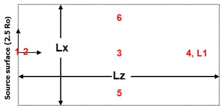
Two directions, z and x, are simulated, as depicted in Fig. 1. The directionzis the longitudinal or streamwise di-rection, oriented away from the Sun. Open boundary condi-tions are set atz=0 and z=Lz, the domain length in the zdirection. In the transverse or cross-stream directionx re-flecting boundary conditions are set. All three velocity ponents are retained. The following viscous-resistive com-pressible MHD equations in dimensionless form, written in the Lagrangian frame, are solved:
Fig. 1. Sketch of the domain simulated with FLIP-MHD. The left boundary corresponds to the source surface, conventionally located at 2.5 solar radii. The right boundary is placed at the terrestrial at-mosphere.LxandLzare the box size in thexandzdirections. The red numbers mark the diagnoses locations, as explained in Sect. 3.
Mass continuity: ∂ρ
∂t = −∇ ·ρv (1)
Momentum equation:
ρ∂v
∂t = −ρ (v· ∇)v− ∇p− "
∇|B|
2
2 −(B· ∇)B #
+ 1
<ν1v (2)
Magnetic flux equation (Faraday’s law): ∂B
∂t = ∇ ×(v×B)+
1
S1B (3)
Energy equation
ρ∂I
∂t = −p∇ ·v+ (∇ ·v)2
<λ +
Q·Q
<ν +
J·J
S , (4)
whereρ is the mass density,B is the magnetic field which obeys the Gauss law constraint∇ ·B=0,vis the fluid veloc-ity,I is the specific internal energy,J is the current density, p is the fluid pressure, andQthe symmetric rate-of-strain tensor defined as
Y
=1
2 h
∇v+ ∇vTi. (5)
In Eqs. (2)–(4)<λand<ν are the Reynolds numbers mea-suring respectively the global kinematic and dynamic vis-cosity in the numerical box; in the simulations shown,<λ
=<ν = 103is always assumed. The quantityS=103is the Lundquist number measuring the global explicit resistivity set within the domain.
2.1 Definition of the source function
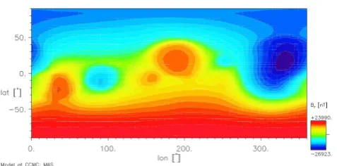
Fig. 2. Example of an extrapolated magnetic field at the source sur-face. From CCMC, http://ccmc.gsfc.nasa.gov.
at a distance of 2.5 solar radii from the solar surface. The boundary conditions at the source surface are in turn obtained from observations at the photosphere, such as GONG magne-togram synoptic maps. Figure 2 shows an example of the ex-trapolated magnetic field at the source surface obtained using the MAS tool (Riley et al., 2001) at the Community Coordi-nated Modeling Center, CCMC (http://ccmc.gsfc.nasa.gov).
In this paper, the FLIP-MHD model is driven by a syn-thetic analytical function providing the input conditions for the magnetic and velocity fields at the source surface. For simplicity, the velocity at the source surface is taken as con-stant. Instead, the boundary condition for thezcomponent of the magnetic field at the source surface is imposed as follows:
bz=b0tanh(x−xcentre)+ b0 f (t )sin
2π(x−x centre) LB
(6)
xcentreis the middle point of the domain in thexdirection. The equations solved in the code and reported in the results below use normalised units. The magnetic field is normalised tob0, the unit length is defined by the thicknessLB, and the unit time is computed as the time required by an Alfvén wave to travel one unit distance LB, the so-called Alfvén time: τA=LB/vA. Note that in this choice of units the reference Alfvén speed isvA=1.
The magnetic field at the source surface varies in time as determined by the functionf (t )defined as
f (t )=
0.5(1−cos(π(1−t /tα))t < tα
1 Otherwise (7)
tα=tfinal·α. The maximum value oftα is reached before the final time,tfinal/τA=400, when alpha is less then 1. In par-ticular, we select a valueα=0.4, to introduce an initial phase of dynamic perturbation and subsequently observe the relax-ation of the system to a constant drive.
Theyandxcomponents of the magnetic field and the ve-locity in the longitudinal direction are selected to ensure an initial force-free equilibrium (that is, no force is acting on
the plasma): by= −
b0 cosh(x_xcentre)
, (8)
bx=0, (9)
and
u=1. (10)
With these boundary conditions, the evolution of the so-lar wind magnetic field and velocity is studied between the source surface and 1 AU.
The real heliospheric case is of course spherical. However, a full 3-D description is beyond the scope of the present pa-per that aims instead at ascertaining the sensitivity of MHD models to boundary drives. For this reason and at the cost of losing the effects of the geometric expansion, a Cartesian grid is used instead. Figure 1 shows the domain used. Lx andLz are the system dimensions in the cross stream wise and stream wise direction respectively. The out of planey di-mension is assumed ignorable. In code units,Lx/LB=3.6 andLz/LB=98.4. The red numbers mark the diagnoses lo-cations defined later in Sect. 3.
The solar wind speed is assumed to be Alfvénic,VSW= VA, at the injection boundary, and the total simulation time allows roughly 4 transit times in thezdirection. When com-pared with the real heliospheric case, the distanceLz repre-sents the Sun to Earth distance and therefore the total sim-ulation time corresponds to approximately 4 times the total time required for the solar wind to reach the Earth. For typ-ical solar wind speeds this corresponds to roughly 12 days. Of course, given the choice of a Cartesian grid this is only an indicative number.
3 Methodology
The model sensitivity analysis consists in describing the un-certainties of a reference simulation from a set of simula-tions over a chosen time period. Information about both the reliability of the model and about which input parameters contribute most to the variability of the model response is provided through such analysis. From the ensemble method (Evensen, 2009), ensemble variances and ensemble covari-ances can help improve the knowledge of how boundary con-ditions affect the evolution of the system and which areas are particularly sensitive to their variations. This could be help-ful for the identification of the areas where dedicated obser-vations may be useful for the data assimilation process.
ensemble technique is widely used to characterise the inac-curacies in the initialisation of the state of atmospheric and oceanographic forecasting models.
Several initial states are obtained by imposing small varia-tions on top of the initial condivaria-tions. Then, starting from each of these initial states, calculations for future states are made. At a given time, all of the calculated states can be represented by a dispersion or probability distribution.
One of the preliminary steps before applying DA to a model is to derive this probability distribution of the state vector. It can be obtained through a Monte Carlo sampling method which describes the uncertainties with respect to a reference simulation of a set of similar simulations over a chosen period of time. The error covariances can thus be specified. The sample characterises the sensitivity of the model forecast to parameter errors around the current state of the system. Based on this ensemble technique, sensitivity analysis and representers study constitute the cornerstone of the approach presented here, leading to the preliminary un-derstanding of how much DA will be effective.
The analysis includes three main stages:
1. an ensemble of 100 members is generated by perturb-ing the source function as described in Eq. (6); 2. the integration of the FLIP-MHD model over this set
of perturbed initial states provides access to a set of model solutions, representing the probability density of the model state (model errors and uncertainties); 3. diagnoses on the simulated sets are conducted around
some specific locations such as the Lagrange point L1 (location 4), near the source surface (location 2), in the middle of the domain (location 3) and to both sides of the longitudinal axis near the borders of the domain study (locations 5 and 6) (see Fig. 1).
In Sect. 3.1 more information regarding the generation of the perturbations is provided, while in Sect. 3.2, the ensemble diagnostic statistical tools are introduced in greater detail. 3.1 Generation of perturbations
Within the framework of this study, evolved forecast error covariances are constructed using an ensemble of model runs that start from perturbed initial states. Perturbations are built by adding uncertainty to the synthetic source surface mag-netic field inputs in the streamwisezdirection. The velocity, instead, is kept constant.
IfF (x, t )is the analytical function at the source surface, a particular perturbed fieldFpert(x, t )is obtained as in Fpert(x, t )=F (x, t )+γ (t )F (x, t ), (11) whereγ (t )is a time-dependent coefficient generated from a Gaussian distribution with mean zero and standard deviation of 0.05. An error of about 5 % with respect to the reference field is imposed.
For each member of the ensemble, the simulation is carried out for 100 time steps up to a final time oftfinal/τA=400. 3.2 Ensemble theory and statistical tools
In this section the ensemble statistical tools used in this study are presented in detail. The concepts of representers tech-nique and domain of influence are introduced, based on the ensemble Kalman filter method.
3.2.1 Ensemble Kalman filter and representers
The representers technique has been used widely for oceanic or tidal circulation problems as reported in the literature (Bennet, 1992; Egbert and Bennet, 1996; Lyard, 1999; Echevin et al., 2000; Evensen, 2009). At this stage of the preliminary analysis, it is a simple and robust tool for in-vestigating how the system with DA will spatially propagate the information brought by dedicated observations and how strong the correlation between the observation taken at a par-ticular spatial location and the other grid points is. A brief summary of the ensemble Kalman filter technique is pro-vided here with the aim of facilitating the reading of the rest of the paper.
In the framework of the ensemble Kalman filter, a series of forecasting and analysis steps are executed in a sequence. First, the forecasting step provides model predictions from the last analysis state and calculates the forecast errors of the model by propagating the analysis errors appropriately.
Then the analysis step at time ti corrects the forecasted statexf(ti)with the information obtained from the observa-tion vectoryo (ti). The corrected statexa (ti)is calculated according to the following formula:
xa(ti)=xf(ti)+K(ti) h
yo(ti)−H(ti)xf(ti) i
, (12) wherexf(ti)is the forecast of the state at time ti,yo(ti)is the vector of observations at the same time and the matrix H(ti)is the so-called “observation operator”. It ensures the projection of the model space onto the observation space. In this particular case, the state vectorxincludes the solar wind magnetic and velocity fields at all grid points of the simu-lated domain;yo(ti)−H(ti)xf(ti)is the “innovation” matrix, which carries the information relative to the difference be-tween the actual observations and the corresponding values for the forecasted fields; K(ti)is the Kalman gain matrix at timeti, given by:
K(ti)=Pf(ti)HT(ti) h
H(ti)Pf(ti)HT(ti)+r(ti) i−1
Malanotte-Rizzoli, 1991; Bouttier and Courtier, 1999). The matrix K(ti)weights the forecast and the observations ac-cording to their respective error statistics, Pf(ti)and r(ti). Notice that Eqs. (12) and (13) are recalled to provide a gen-eral background to the Kalman filtering procedure used for data assimilation: indeed, the actual assimilation of helio-spheric observations has not been carried out yet. The present work focuses in fact on the concept of representers, which is described below. The rest of this section aims at explaining the role of the representer matrices in this sensitivity study without actually performing the assimilation procedure and without having observations at our disposal.
Representers or influence functions are obtained by refor-mulating the analysis step of the Kalman filter described in Eq. (12), as in
xa(ti)=xf(ti)+ j=pi
X j=1
bj(ti)rj(ti), (14)
wherexf(ti)is the forecasted state vector at timeti, rj(ti)is the representer or influence function relative to thejth obser-vation at timeti andpi is the number of observations avail-able at timeti. The representer rj(ti)is a vector which has the dimensions of the state vector andbj(ti)is the scalar co-efficient associated with the observationjat timeti.
Equation (14) translates in matrix form into
xa(ti)=xf(ti)+r(ti)b(ti), (15)
with the matrix r(ti)defined at timeti as
r(ti)=Pf(ti)HT(ti), (16)
and the vectorb(ti)as
b(ti)= h
H(ti)Pf(ti)HT(ti)+r(ti) i−1
h
yo(ti)−H(ti)xf(ti) i
. (17)
The matrix r(ti)contains as many columns as there are ob-servations available at timeti and each column constitutes the representer rj(ti) relative to a given observation. The representer formulation of the analysis step of Eq. (14) can be interpreted as the correction of the forecasted statexf(ti) done by using a combination of representers, depending on the forecast error covariance matrix Pf(ti). Note that in the case of a multivariate state vector (e.g. solar wind magnetic and velocity fields), the information from thejth observation can be spread to the other model state variables, thanks to the error cross-covariance of these variables.
Notice that from this point onwards, the time dependence is dropped for ease of reading. It is also assumed that the model grid is composed ofnnodes and that the state vec-tor contains two variables (namely magnetic field and solar wind velocity). The dimension of the state vector is then 2n.
Now, focusing on a single observation, Eq. (16) becomes, at a given time:
rj=PfHTj (18)
Hjis the raw of the matrix H corresponding to thejth obser-vation. For the purpose of the demonstration, let us assume that thejth observation is (1) exactly located at a grid point k and (2) associated with one of the state vector variables. Thus, this observation is identified in the state vector by its indexkj. Then, Hj (kj)is the only non-zero element of Hj, that is
Hj=(0, . . .,0,1,0, . . .,0), (19) with only one “1” at indexkj. Thus, Eq. (18) gives, from the definition of Pf,
rkj=P fHT
kj =
cov(εfk
j, ε f 1) .. . cov(εfk
j, ε f n) cov(εkf
j, ε f n+1) .. . cov(εfk
j, ε f 2n)
(20)
εf is the model forecast error, defined as the difference be-tween the forecasted and true states (xf−xt), which is not known. The abbreviation “cov” stands for “covariance”.
Consequently, the representer of observation j contains the covariances between the model forecast errors at the ob-servation point and all the grid nodes, for all the state vari-ables (e.g. magnetic field, solar wind velocity).
As explained in Sect. 3, the model forecast errors can be estimated through the stochastic modelling approach: if an ensemble of simulations generated by perturbing one or sev-eral sources of errors of the model is available, these model forecast errors are approximated by statistics computed from this ensemble. Thus, the covariances of the model forecast er-rors are estimated by the ensemble covariances of the model forecast errors. Therefore
cov(εfk
j, ε f i)≈cov
ens(εf kj, ε
f i) = 1 m m X s=1
(εfk
j,s−
1 m
m X s=1
εkf
j,s)(ε f i,s− 1 m m X s=1
εfi,s)
=(εfk
j−ε f kj)(ε
f
i−εfi), (21)
unbiased. This implies that cov(εkf
j, ε f
i)≈(εfkj)(ε f i)
≈(xfk
j−x f kj)(x
f i−x
f i)
≈cov(xfk
j,x f
i). (22)
Thus, more generally, the variances, covariances and corre-lations of the model forecast errors are identifiable as the en-semble variances, covariances and correlations of the state variables.
3.2.2 Domain of influence of a single observation
Here an explicit expression for the domain of influence of a single observation is presented. Consider an isolated obser-vationykj relative to the forecasted state variablex
f (mag-netic field components or solar wind velocity components) and located on a nodekof the mesh. The correction applied on the forecasted statexf calculated by assimilation of the observationykj is expressed by
δx=xa−xf=bkjrkj (23)
with rkj =PfHTk
j=(cov(ε f kj, ε
f
i))i=1,2n (24)
bkj =
ykj−xkj
cov(εfk
j, ε f
kj)+cov(ε o kj, ε
o kj)
= δykj
var(εfk
j)+var(ε o kj)
(25)
whereδykj andε o
kj are respectively the innovation and the
observation error associated with the observationykj; the
ab-breviation “var” stands for the ensemble variance.
Combining Eqs. (23), (24) and (25), the correction at node ibrought by the observationykjis then expressed as follows:
δxi=
cov(εkf
j, ε f i)
var(εfk
j)+var(ε o kj)
δykj (26)
Introducing the formal definition of the correlation, the pre-vious equation becomes
δxi=
cov(εf kj,εfi) r
var(εf kj)var(εfi)
var(εf kj)+var(εokj) r
var(εf kj)var(εfi)
δykj = correl(εf
kj,εfi) 1+
var(εo kj)
var(εf kj)
s var(εfi) var(εf
kj)
δykj
≈correl(xfk
j,x f i) v u u t
var(εf i)
var(εf kj)
1+
var(εo kj)
var(εf kj)
δykj
≈correl(xfk
j,x f
i)×modulation factor(εkoj, ε f kj, ε
f i)δykj,
(27)
where the abbreviation “correl” refers to correlation. Therefore, the correction at pointi, obtained by the assim-ilation of the isolated observationykj, depends on the
cor-relation between the model forecast errors associated with the observed variable xkj and the variable to be corrected
xi. According to Eq. (22), this correlation is approximated by the ensemble correlation of the observed variablexkj and
the variable to be correctedxi. This correlation term reflects the spatial extent of the correction and thus represents the
domain of influence (hereafter “doi”) of the observationykj.
Note that the magnitude of the correctionδxi is represented by the modulation factor term that depends on the observa-tion error and on the ratio of the model error variances at the pointiand at the observation pointk: if the observation error is strong, the correction has to remain low; if the model error variance is higher/lower at the pointithan at the observed point, the correction must be significant/lower.
As a first step in the implementation of a dedicated DA system, this study will focus on the doi of isolated observa-tions (magnetic or solar wind velocity fields) rather than on the modulation factor.
4 Results on ensemble statistics
In this section the statistical ensemble variance and domain of influence analysis outlined above are presented. With these experiments, we inspect the potential impact of the DA technique on the improvement of the state at the source sur-face and, more in general, on the entire simulated domain. All parameters (spatial, time, magnetic and velocity field) in the paper should be considered normalised to the normalisa-tion factors described earlier in Sect. 2.1.
4.1 Gaussian character of error statistics
For the model error statistics exploration process of this study, a set of 100 ensemble members is generated. This number is usually chosen for stochastic modelling to ensure a statistical significance at a reasonable computational cost.
When implementing real DA experiment it should be nec-essary to conduct a convergence analysis to determine the optimal number of members leading to a sufficient stability of the statistics computed from the ensemble members.
The Gaussian nature of the perturbed states is very impor-tant for the data assimilation schemes since it ensures that the optimal state calculated in the analysis step is the most probable in the sense of maximum likelihood. In the context of ensemble methods, the forecast error of the model can be estimated from the dispersion of the perturbed model trajec-tories around the overall average at a given time step.
30 1
2
Figure 3. Distribution of the forecast errors for the z component of the solar wind velocity and 3
magnetic field at the different test locations illustrated in figure 1: location 1 (source surface), 4
location 2, location 3, location 4 (Lagrange point, L1), location 5 and location 6. The errors are 5
calculated from the dispersion of the perturbed ensemble member trajectories around the 6
ensemble average. 7
8
9
10
11
12
13
14
15
16
17
Fig. 3. Distribution of the forecast errors for thezcomponent of the solar wind velocity and magnetic field at the different test locations illustrated in Fig. 1: location 1 (source surface), location 2, location 3, location 4 (Lagrange point, L1), location 5 and location 6. The errors are calculated from the dispersion of the perturbed ensemble member trajectories around the ensemble average.
the information relative to all the ensemble members at all the time steps available. These histograms are thus com-puted on a sample of 10 000 (100 members times 100 out-puts) achievements and show the empirical distributions of the model error as a function of the perturbed source surface input.
It can be noted that the shape of the error distribution is slightly broader for locations 4, 5 and 6 compared to loca-tions 1, 2 and 3. This is due to a higher level of non-linear interactions and unsteady state conditions further away from the source surface.
Overall, the sampling distributions can be fitted, in a first approximation, with a quasi-Gaussian. This ensures that the BLUE (cf. Sect. 3.2) hypothesis can be made and that the classical formulation of data assimilation, on which the present study relies, is pertinent. However, it should be men-tioned that some reconnection events are triggered in some ensemble members. This could explain, at some locations, the deviation from the Gaussian shape of the distribution of the errors.
4.2 Ensemble variances
As part of the sensitivity study, ensemble variance diagnoses for the magnetic field and velocity at the previously desig-nated locations of the domain are discussed. The objective is to estimate the error structures of the model, in order to point out the areas where gathering dedicated observations may be useful. In this framework, the model response to perturba-tions of the boundary condition inputs at the source surface has been calculated. This will highlight the areas where phys-ical processes are poorly modelled and will also allow esti-mating of the reliability of the model. In the first subsection, the temporal evolution of the ensemble variances is analysed
31 1
Figure 4. : Time evolution of the ensemble variance for the normalized bz (left panels) and time evolution of the
2
normalized bzfor all the ensemble members (right panels) at the selected diagnosis locations. The red curve
3
represents the average of the ensemble and the green curve refers to the reference simulation, where no perturbation 4
is applied to the source surface inputs. bzis normalized to b0 and the time to the Alfvén time A. Note that the
5
left and right bzscales are not common to the six diagnosis points.
6
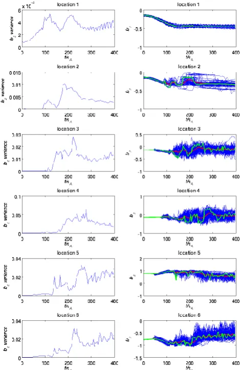
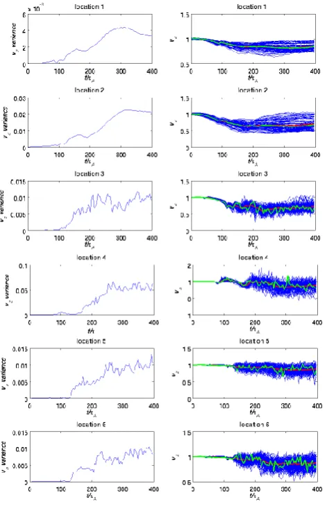
Fig. 4. Time evolution of the ensemble variance for the normalised bz(left panels) and time evolution of the normalisedbzfor all the ensemble members (right panels) at the selected diagnosis loca-tions. The red curve represents the average of the ensemble and the green curve refers to the reference simulation, where no perturba-tion is applied to the source surface inputs.bzis normalised tob0 and the time to the Alfvén timeτA. Note that the left and rightbz scales are not common to the six diagnosis points.
at fixed points in space. In the second subsection, the spatial structures of the ensemble variances are studied in the whole domain simulated.
4.2.1 Local temporal evolution of ensemble variances
32
Figure 5. Time evolution of the ensemble variance for the normalized vz (left panels) and time evolution of vz
1
for all the ensemble members (right panels) at the selected diagnosis locations. The red curve represents the 2
average of the ensemble and the green curve refers to the reference simulation, where no perturbation is applied 3
to the source surface inputs. vzis normalized to the Alfvén speed vA and the time to the Alfvén time A. Note
4
that the left and right vzscales are not common to the six diagnosis points.
5
Fig. 5. Time evolution of the ensemble variance for the normalised vz(left panels) and time evolution ofvzfor all the ensemble mem-bers (right panels) at the selected diagnosis locations. The red curve represents the average of the ensemble and the green curve refers to the reference simulation, where no perturbation is applied to the source surface inputs.vzis normalised to the Alfvén speedvAand the time to the Alfvén timeτA. Note that the left and rightvzscales are not common to the six diagnosis points.
and their associated maps of evolution for all of the ensem-ble members (right panels), for six representative locations chosen in the whole domain as depicted in Fig. 1. In the right panels, the red curve represents the temporal evolution of the ensemble average, while the green curve refers to the ref-erence simulation whose source surface input is left unper-turbed.
Considering the rate of perturbation that has been applied in this stochastic modelling, one can see that the evolution of the variability in the ensemble remains quite admissible and maintains fairly reasonable error bounds for bothbzandvz.
Except for location 1 near the source surface, where the variance remains very low, it can be noted here that the en-semble variance evolution is quite similar for the six
loca-tions: the variance of the ensemble is extremely low at the beginning of the time series. Reasonably, though, the loca-tions far from the source surface show slightly higher differ-ences in the evolution than the closer ones, as depicted in the right panels of Figs. 4 and 5. At later time steps,t /τA≈88 for location 2,t /τA≈120 for location 3,t /τA≈140 for lo-cations 5 and 6 andt /τA≈160 for location 4, the variance starts increasing for all of the locations: the ensemble expe-riences rather different evolutions. These differences in the time evolution of the ensemble variances are the signature of a dynamical process which crosses the domain from the source surface to L1.
This notwithstanding, it can be noticed that ensemble av-erages and reference simulations behave quite similarly; this confirms that the stochastic modelling protocol is mostly lin-ear, and thus corroborates the quasi-Gaussian feature of the distribution of the errors stated in Sect. 4.1.
4.2.2 Spatial structure of the ensemble variance
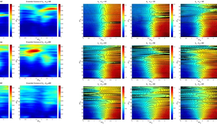
Fig. 6. Ensemble variance of the normalisedzcomponent of the magnetic field at different time steps and on the entire simulated domain. The spatial dimensions are normalised toLB, the length scale of variation of the magnetic field. Time is normalised to the Alfvén timeτA.
The simulation instances reconnecting “together” (i.e. at sim-ilar time and space) are presumably the ones excited with a similar magnetic field at the boundary.
4.3 Domains of influence
The study of the ensemble variance of the model allowed one to describe how the physical fields respond differently to a perturbation of the model inputs and to characterise the model forecast error. The ensemble modelling protocol that has been set up in the present study provides an efficient way of investigating the model forecast error covariances. These covariances indeed play a leading role in the problem of data assimilation since they ensure the propagation of the infor-mation provided by the observations to all model variables. Therefore they determine the spatial extent and magnitude of the state corrections provided by the assimilation of tions. Here the objective is indeed to illustrate how observa-tions taken at a measurement point located in one particular position of the domain would affect the overall model evolu-tion if those observaevolu-tions were assimilated into the model.
For real heliospheric application, the availability of ob-servation points is currently very limited. The main obser-vation point is the ACE spacecraft located at L1 position corresponding to location 4 in this study. As mentioned be-fore, additional important information can be obtained by the STEREO mission.
In Fig. 8, the panels illustrate the domain of influence “doi” as defined in Eq. (27), forbz, for observations taken at different locations. The effects of reconnection at the
dif-Fig. 7.zcomponent of the magnetic field and, superimposed, the field lines for the reference simulation at different time steps and on the entire simulated domain. The spatial dimensions are normalised toLB, the length scale of variation of the magnetic field. Time is normalised to the Alfvén timeτA,bzis normalised tob0.
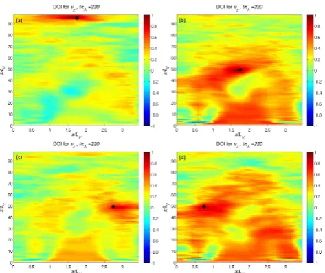
Fig. 8. Domain of influence for thezcomponent of the magnetic fieldbz for the assimilation of a magnetic field observation made at different locations at the same time step,t /τA=220. The black circle indicates the data observation location. (a) refers to location 4 (L1, 1 AU), (b) to location 3, (c) to location 5 and (d) to location 6. The spatial dimensions are normalised toLB, the length scale of variation of the magnetic field; time is normalised to the Alfvén timeτA.
ferent locations of the simulation domain (see Fig. 1) and at different times are shown.
Fig. 9. Domain of influence for thezcomponent of the solar wind velocityvz for the assimilation of a velocity observation taken at different locations at the same time stept /τA=220. The black cir-cle indicates the data observation location. (a) refers to location 4 (L1, 1 AU), (b) to location 3, (c) to location 5 and (d) to location 6. The spatial dimensions are normalised toLv=LB, the length scale of variation of the velocity; time is normalised to the Alfvén timeτA.
and the domain of influence are referred to thezcomponent of the magnetic field.
Notice that the amplitude of the correlation at the obser-vation point location is equal to “1”, which is the maxi-mum positive correlation. Then, the correlation progressively decreases when moving away from the observation point. When the ensemble correlation approaches the maximum negative correlation, value “−1”, degradation may occur. This can actually happen when moving too far away from the observation area. In this case, when implementing DA tech-nique, the analysis step should be restricted to the area with positive correlation. As explained in Sect. 3.2.2, the correla-tions here reflect the potential spatial extent of the correction around a given location with an isolated observation. Then, the correlation amplitude (Eq. 27) will be modulated, taking into account the observation error (with strong observation errors, the model correction remains low) and the ratio of er-ror variances at the point to be corrected (correction could be significant or lower).
Notice that the domain of influence of the observation is rather localised and decreases to 0 when moving towards the Sun. This result makes sense, since the driver of the simula-tion is located at the source surface, i.e. far away from the L1 location, and means that observations of the magnetic field taken at L1 can only slightly improve the model evolution closer to the source surface.
It is also important to observe that the occurrence of mag-netic reconnection results in the fact that some regions of the
domain remain magnetically isolated. The beneficial feed-back from assimilation is thus prevented from spreading into those regions. This effect is particularly severe for the obser-vations taken at L1.
The doi plots from Fig. 8 for location 3 (panel b), loca-tion 5 (panel c) and localoca-tion 6 (panel d) respectively, which again refer to the space and time evolutions of the domain of influence of various magnetic field observations, show more reassuring results: observations taken at those locations would significantly improve the model structure at greater distances, thus making the use of data assimilation a worthy tool for making the model evolution closer to reality. Notice again that the influence of an observation point on the rest of the domain is strictly bound to the occurrence of tion, which temporarily magnetically isolates the reconnec-tion area from the rest of the domain. Note that these findings are independent of time and remain similar throughout the whole period.
The same doi analyses are performed for the solar wind velocityvz. Figure 9 shows the domain of influence for the solar wind velocity in the case of the assimilation of a veloc-ity observation made at location 4 (panel a), location 3 (panel b), location 5 (panel c) and location 6 (panel d) respectively at timet /τA≈220. Notice that the correlation impact is wider than for magnetic field measures and extends over time to cover the simulation domain entirely, as visible in Fig. 10, which refers to the same spatial locations but to a later time, t /τA≈344. This ensures that data assimilation would signif-icantly minimise the model errors in the velocity field when velocity observations are assimilated. Panel (a) is of particu-lar relevance, since it shows that observations taken at 1 AU, where most of the space weather relevant satellites are lo-cated, also have a very strong effect in improving the solar wind velocity representation over almost the entire domain.
The results thus show that data assimilation should im-prove the forecast of velocity and magnetic fields not only near and around the observation location, but also for grid points rather far from the measurement location.
It is reminded that, as from Eq. (14), the correction of the forecasted state is a linear combination of represen-ters associated with the observations assimilated. The rep-resenters include both contributions from covariances for the same fields (magnetic field or velocity field) and from cross-covariances between different fields (magnetic field with ve-locity field): each representer propagates information from the observation to the different variables of the state vector. This means, in this case, that assimilation of magnetic field observations might improve the state for the solar wind ve-locity as well, and vice versa.
Fig. 10. Domain of influence for thezcomponent of the solar wind velocityvz for the assimilation of a velocity observation taken at different locations at the same time stept /τA=334. The black cir-cle indicates the data observation location. (a) refers to location 4 (L1, 1 AU), (b) to location 3, (c) to location 5 and (d) to location 6. The spatial dimensions are normalised toLv=LB, the length scale of variation of the velocity; time is normalised to the Alfvén timeτA.
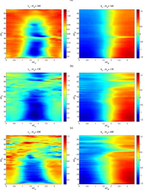
Fig. 11. Domain of influence for thezcomponent of the solar wind velocityvzfor the assimilation of a magnetic field observation taken at different locations and different times. The black circle indicates the data observation location. (a) refers to location 4 (L1) and time t /τA=176, (b) to location 3 and timet /τA=140, panel (c) to lo-cation 5 and (d) to lolo-cation 6, both at timet /τA=228. The spatial dimensions are normalised toLv=LB, the length scale of variation of the velocity; time is normalised to the Alfvén timeτA.
throughout the simulation at different time steps. It should be noted that only specific cases are shown. The less interesting
Fig. 12.zcomponents of the solar wind velocityvz(left panel) and of the magnetic fieldbz(right panel) of the reference simulation in correspondence with doi plots of Fig. 11, for times (a)t /τA=176, (b)t /τA=140 and (c)t τA=228. The spatial dimensions are nor-malised toLv=LB, the length scales of variation of the magnetic field and of the velocity; time is normalised to the Alfvén timeτA. bzis normalised tob0andvzis normalised to the Alfvén speedvA.
cases with no correlation are dropped. For both locations 4 and 3 the domain of influence is characterised by the appear-ance of a dipole around the observation location with a sep-aration of correlated and anti-correlated areas. For location 6 the doi shows an anti-correlated area, while for location 5 the doi is characterised by a positive ensemble correlation. As a reference, Fig. 12 shows thezcomponents of the solar wind velocity vz (left panel) and of the magnetic fieldvz (right panel) of the reference simulation for the same times of the doi plots of Fig. 11. Preliminarily, this figure indicates that the cross correlations are related to the sign of the magnetic and velocity fields, respectively.
Fig. 5 (right panels), the behaviour ofbzat the different loca-tions is more complicated. From the right panels of Fig. 4 it is possible to notice that at locations 4 and 3, where dipoles are present in Fig. 10, some of the ensemble members ex-hibit positive values of bz, while the rest of the ensemble members experience negative values of the magnetic field. At location 6, where most of the domain shows negative cor-relation, all the ensemble members have negative magnetic fields. At location 5, which is mostly positively correlated, bzis positive for all the ensemble members.
Further studies need to be conducted to better understand this behaviour.
5 Conclusions
Investigations were made to assess if and how the use of data assimilation techniques could lead to more accurate esti-mates of state variables (i.e. solar wind velocity and magnetic field) for solar wind models in different regions of the helio-sphere. A location of particular interest is the source surface, since boundary conditions for solar wind models are usu-ally taken there. More in general, the potential domains of influence due to assimilation of virtual measurements taken at different locations of space on the evolution of the FLIP-MHD model for the solar wind were investigated. The gen-eral aim of the study was to understand the processes and dy-namics in terms of spatial and temporal features of an MHD heliospheric model. A sensitivity study has been conducted through ensemble variances and representer “influence func-tions” analysis, both performed with multiple runs of the model on statistically guided modifications of the input.
First, the sensitivity study permits us to characterise the sensibility of the model to the variation of the input param-eters. This allowed us to better identify the reaction of the model to small variations in the boundary conditions. It is now understood how minimal differences in the boundaries may give rise to a different pattern of reconnection events and that, as a consequence, a faithful representation of the source surface conditions is paramount for the evolution of such models. Hence, the necessity of reliable boundary conditions arises. Another result is the estimate of the error structures of the model, which helps to emphasise the domain areas where dedicated observations may be useful to be collected.
Second, the representer analysis has been used to antic-ipate and estimate the potential contribution of DA to the model evolution. Indeed, the ensemble modelling led us to investigate the model error covariances with the aim of iden-tifying the potential domains of influence through the assim-ilation of one virtual observation. Such an analysis was per-formed by computing the ensemble correlations and cross correlations, both for magnetic field and velocity measure-ments at different spatial locations. It was shown that, while for magnetic field measurements the model improvement is rather bound to the location of the observation and also to
the occurrence of magnetic reconnection, the assimilation of velocity measures grants model benefits which span fur-ther away from the observation location in space and which are less affected by the occurrence of reconnection. Velocity measurements taken at L1 proved to be strongly correlated with the model evolution, also at large distances.
It should be remarked that calculating ensemble correla-tions also has the advantage of considering the observacorrela-tions one by one, thus isolating the influence of each observation in incrementing the correction. In the intermediate goal of optimising a monitoring network for space weather events, this approach is very interesting and helpful. Indeed, the do-main of influence analysis can already provide useful infor-mation about the spatial extent of the expected correction ob-tained by assimilating one isolated observation. This allows one to identify the spatial coverage required for the design of a space weather observation network.
The approach and the results presented here do not assess the success or the failure of the assimilation system. How-ever, the positive results obtained by computing the domains of influence of virtual observation are a further hint of the po-tential benefits of DA on space weather MHD models. The next step would be to implement and run the complete DA, by applying the correction brought by the observations to the forecasted statexf(Eq. 14).
From this study, two main strategies for applying DA to heliospheric models emerge. One consists in updating di-rectly the model fields in the simulation space. If magnetic field values are updated, special attention must be dedicated to the solenoidal condition for the magnetic field. The other one consists in correcting the boundary values at the source surface in order to feed the model continuously with optimal boundary conditions. The study focused on the second strat-egy, since poor magnetograms are known as a major source of errors in ambient solar wind modelling.
Acknowledgements. The authors thank their colleagues for
contin-uing support and discussion. The research leading to these results has received funding from the European Commission’s Seventh Framework Programme (FP7/2007-2013) under grant agreement eHeroes (project no. 284461, www.eheroes.eu). Figure 2 has been provided by the Community Coordinated Modeling Center at Goddard Space Flight Center through their public Runs on Request system (http://ccmc.gsfc.nasa.gov). The CCMC is a multi-agency partnership between NASA, AFMC, AFOSR, AFRL, AFWA, NOAA, NSF and ONR. The MAS model was developed by J. Linker, Z. Mikic, R. Lionello, P. Riley, N. Arge and D. Odstrcil at PSI, AFRL, U. Colorado.
Edited by: S. Sharma
References
Baker, D. N.: What is space weather?, Adv. Space Res., 22, 7–16, 1998.
Barrero Mendoza, O., De Moor, B., and Bernstein, D. S.: Data as-similation for magnetohydrodynamics systems, J. Comput. Appl. Mathe., 189, 242–259, 2006.
Beck, A., Innocenti, M. E., Lapenta, G., and Markidis, S.: Multi-level multi-domain algorithm implementation for two-dimensional multiscale particle in cell simulations, doi:10.1016/j.jcp.2013.12.016, 2013.
Bennet, A. F.: Inverse Methods in Physical Oceanography, Mono-graphs on Mechanics and Applied Mathematics, Cambridge Uni-versity Press, Cambridge, 1992.
Bothmer, V. and Daglis, I. A.: Space Weather – Physics and effects, Springer, Praxis Publishing, Chichester, 2007.
Bouttier, F. and Courtier, P.: Data assimilation concepts and meth-ods, Meteorological Training Course Lecture Series, ECMWF, 1999.
Brackbill, J. U.: FLIP MHD – A particle-in-cell method for magne-tohydrodynamics, J. Comput. Phys., 96, 163–192, 1991. Dwivedi, B. N. and Mohan, A.: First tomographic view of coronal
mass ejections, Current Sci., 88, 688–690, 2005.
Echevin, V., De Mey, P., and Evensen, G.: Horizontal and verti-cal structure of the representer functions for sea surface mea-surements in a coastal circulation model, J. Phys. Oceanogr., 30, 2627–2635, 2000.
Egbert, G. D. and Bennett, A. F.: Data assimilation methods for ocean tides, Modern Approaches to Data Assimilation in Ocean Modeling, edited by: Malonotte-Rizzoli, P., Elsevier Science, 147–179, 1996.
Evensen, G.: Data Assimilation: The Ensemble Kalman Filter, 2nd Edn., Springer, Berlin, 2009.
Fleck, B., Domingo, B., and Poland, A. I.: The SOHO Mission, Solar Phys., 162, 1–531, 1995.
Gantois, K., Santandrea, S., Teston, F., Strauch K., Zender, J., Tilmans, E., and Gerrits, D.: Big year for small satellite – ESA’s second in-orbit technology demonstrator mission: PROBA-2, ESA Bulletin, 144, 22–33, 2010.
Ghil, M. and Malanotte-Rizzoli, P.: Data assimilation in meteorol-ogy and oceanography, Adv. Geophys., 33, 141–266, 1991. Gosling, J. and Pizzo, V.: Formation and evolution if corotating
interaction regions and their three dimensional structure, Space Sci. Rev., 89, 21–52, 1999.
Innocenti, M. E., Lapenta, G., Vrsnak, B., Crespon, F., Skan-drani, C., Temmer, M., Veronig, A., Bettarini, L., Markidis, S., and Skender, M.: Improved forecasts of solar wind pa-rameters using the Kalman filter, Space Weather, 9, 10005, doi:10.1029/2011SW000659, 2011.
Innocenti, M. E., Lapenta, G., Markidis, S., Beck, A., and Va-pirev, A.: A multi-level multi domain method for particle in cell plasma simulations, J. Comput. Phys., 238, 115–140, doi:10.1016/j.jcp.2012.12.028, 2013.
Kalman, R.: A new approach to linear filtering and prediction prob-lems, J. Basic Eng., 82, 35–45, 1960.
Kondrashov, D., Shprits, Y., Ghil, M., and Thorne, R.: A Kalman filter technique to estimate relativistic electron lifetimes in the outer radiation belt, J. Geophys. Res., 112, A10227, doi:10.1029/2007JA012583, 2007.
Laakso, H., Taylor, M. G. G. T., and Escoubet, C. P.: The Cluster active archive – Studying the Earth’s space plasma environment, Springer, Astrophysics and Space Science Proceedings, 2010. Levine, R. H., Altschuler, M. D., and Harvey, J. W.: Solar Sources
of the Interplanetary Magnetic Field and Solar Wind, J. Geophys. Res., 82, 1061–1065, 1977.
Lyard, F.: Data assimilation in a wave equation: a variational repre-senter approach for the Grenoble tidal model, J. Comput. Phys., 149, 1–31, 1999.
McComas, D. J., Bame, S. J., Barraclough, B. L., Feldman, W. C., Funsten, H. O., Gosling, J. T., Riley, P.; Skoug, R., Balogh, A., Forsyth, R., Goldstein, B. E., and Neugebauer, M.: Ulysses’ re-turn to the slow solar wind, Geophys. Res. Lett., 25, 1-4, 1998. Odstrcil, D.: Modeling 3-D solar wind structure, Adv. Space Res.,
32, 497–506, 2003.
Pesnell, W. D., Thompson, B. T., and Chamberlin, P. C.: The Solar Dynamics Observatory (SDO), Solar Phys., 275, 3–15, doi:10.1007/978-1-4614-3673-7_2, 2012.
Rigler, E., Baker, D., and Weigel, R.: Adaptive linear prediction of radiation belt electrons using the Kalman filter, Space Weather, 2, S03003, doi:10.1029/2003SW000036, 2004.
Riley, P., Linker, J. A., and Mikic, Z.: An empirically-driven global MHD model of the solar corona and inner heliosphere, J. Geo-phys. Res., 106, 15889–15901, 2001.
Schunk, R. W., Scherliess, L., and Sojka, J. J.: Recent approaches to modeling ionospheric weather, Adv. Space Res., 31, 819–828, 2003.
Schunk, R. W., Scherliess, L., Sojka, J. J., Thompson, D. C., An-derson, D. N., Codrescu, M., Minter, C., Fuller-Rowell, T. J., Heelis, R. A., Hairston, M., and Howe, B. M.: Global Assim-ilation of Ionospheric Measurements (GAIM), Radio Sci., 39, doi:10.1029/2002RS002794, 2004.
Schrijver, C. J. and Derosa, M. L.: Photospheric and heliospheric magnetic fields, Solar Phys., 212, 165–200, 2003.
Sheeley, N. R. and Harvey, J. W.: Coronal holes, solar wind streams, and geomagnetic disturbances during 1978 and 1979, Solar Phys., 70, 237–249, 1981.
Siscoe, G.: The space-weather enterprise: past, present, and future, J. Atmos. Solar-Terrest. Phys., 62, 1223–1232, 2000.
Stone, E. C., Frandsen, A. M., Mewaldt, R. A., Christian, E. R., Margolies, D., Ormes, J. F., and Snow, F.: The Advanced Com-position Explorer, Space Sci. Rev., 86, 1–22, doi:10.1007/978-94-011-4762-0_1, 1998.
Toth, G., Sokolov, I. V., Gombosi, T. I., Chesney, D. R., Clauer, C. R., De Zeeuw, D. L., Hansen, K. C., Kane, K. J., Manchester, W. B., Oehmke, R. C., Powell, K. G., Ridley, A. J., Roussev, I. I., Stout, Q. F., Volberg, O., Wolf, R. A., Sazykin, S., Chan, A., Yu, B., and Kta, J.: Space weather modeling framework: A new tool for the space science community, J. Geophys. Res., 110, A12226, doi:10.1029/2005JA011126, 2005.
Turner, D. L. and Li, X.: Using spacecraft measurements ahead of Earth in the Parker spiral to improve terres-trial space weather forecasts, Space Weather, 9, S01002, doi:10.1029/2010SW000627, 2011.
Vršnak, B., Temmer, M., and Veronig, A.: Coronal Holes and Solar Wind High-Speed Streams: I. Forecasting the Solar Wind Param-eters, Solar Phys., 240, 315–330, 2007.
Wang, Y. and Sheeley Jr., N. R.: Solar wind speed and coronal flux-tube expansion, Astrophys. J., 355, 726–732, 1990.
Welch, G. and Bishop, G.: An introduction to the Kalman filter, TR 95-041, University of North Carolina, Department of Computer Science, 2001.