Effects of systematic and random errors on the retrieval of particle microphysical properties from multiwavelength lidar measurements using inversion with regularization

www.atmos-meas-tech.net/6/3039/2013/ doi:10.5194/amt-6-3039-2013

© Author(s) 2013. CC Attribution 3.0 License.

Atmospheric

Measurement

Techniques

Effects of systematic and random errors on the retrieval of particle

microphysical properties from multiwavelength lidar measurements

using inversion with regularization

D. Pérez-Ramírez1,2,3, D. N. Whiteman1, I. Veselovskii4, A. Kolgotin4, M. Korenskiy4, and L. Alados-Arboledas2,3

1_{Mesoscale Atmospheric Processes Laboratory, NASA Goddard Space Flight Center, Greenbelt, 20771, Maryland, USA} 2_{Departamento de Física Aplicada, Universidad de Granada, Campus de Fuentenueva s/n, 18071 Granada, Spain}

3_{Centro Andaluz de Medio Ambiente (CEAMA), Universidad de Granada, Junta de Andalucía, Av. del Mediterráneo s/n,}

18006 Granada, Spain

4_{Physics Instrumentation Center of General Physics Institute, Troitsk, Moscow Region, 142190, Russia}

Correspondence to: D. Pérez-Ramírez ([email protected], [email protected])

Received: 2 April 2013 – Published in Atmos. Meas. Tech. Discuss.: 24 May 2013

Revised: 18 September 2013 – Accepted: 30 September 2013 – Published: 7 November 2013

Abstract. In this work we study the effects of systematic and random errors on the inversion of multiwavelength (MW) lidar data using the well-known regularization technique to obtain vertically resolved aerosol microphysical properties. The software implementation used here was developed at the Physics Instrumentation Center (PIC) in Troitsk (Russia) in conjunction with the NASA/Goddard Space Flight Center. Its applicability to Raman lidar systems based on backscattering measurements at three wavelengths (355, 532 and 1064 nm) and extinction measurements at two wavelengths (355 and 532 nm) has been demonstrated widely. The systematic error sensitivity is quantified by first determining the retrieved pa-rameters for a given set of optical input data consistent with three different sets of aerosol physical parameters. Then each optical input is perturbed by varying amounts and the inver-sion is repeated. Using bimodal aerosol size distributions, we find a generally linear dependence of the retrieved errors in the microphysical properties on the induced systematic er-rors in the optical data. For the retrievals of effective radius, number/surface/volume concentrations and fine-mode radius and volume, we find that these results are not significantly affected by the range of the constraints used in inversions. But significant sensitivity was found to the allowed range of the imaginary part of the particle refractive index. Our re-sults also indicate that there exists an additive property for the deviations induced by the biases present in the individ-ual optical data. This property permits the results here to be

used to predict deviations in retrieved parameters when mul-tiple input optical data are biased simultaneously as well as to study the influence of random errors on the retrievals. The above results are applied to questions regarding lidar design, in particular for the spaceborne multiwavelength lidar under consideration for the upcoming ACE mission.

1 Introduction

3040 D. Pérez-Ramírez et al.: Errors of microphysical particle retrievals from 3β+2αlidar measurements

occurring in the atmosphere (Eck et al., 2010) and aerosol dynamics (e.g., Pérez-Ramírez et al., 2012).

Because of these challenges, the characterization of at-mospheric aerosols is being achieved through intense ob-servational programs using remote sensing techniques. For example, NASA has led several spaceborne missions to study aerosol properties worldwide (e.g., the MODIS instru-ment on the TERRA and AQUA platforms). However, satel-lite measurements possess lower temporal resolution than ground-based systems. For example, the AERONET global network (Holben et al., 1998) is providing large data sets of high-temporal-resolution ground-based aerosol measure-ments at more than 400 locations worldwide. But the aerosol retrievals by AERONET and by many satellite platforms only provide column-integrated properties. By contrast, the lidar technique offers vertical profiling of aerosols, from the first lidars in the early 1960s to the more sophisticated Ra-man lidars (WhiteRa-man et al., 1992; AnsRa-mann et al., 1992) or high-spectral-resolution lidars (HSRL) (Shipley et al., 1983; Grund and Eloranta, 1991; She, 2001; She et al., 2001). Moreover, the Nd:YAG laser has been used as the transmit-ter for multiwavelength Raman lidar systems (MW), which have permitted the retrieval of the profile of aerosol micro-physical properties (e.g., Müller et al., 2001, 2004, 2005, 2011; Wandinger et al., 2002; Böckman et al., 2005; Noh et al., 2009; Balis et al., 2010; Alados-Arboledas et al., 2011; Tesche et al., 2011; Veselovskii et al., 2012; Papayannis et al., 2012; Wagner et al., 2013; Navas-Guzmán et al., 2013).

The first attempts to obtain aerosol microphysical prop-erties from MW Raman lidar measurements were done at the Institute for Tropospheric Research (IFT) in Leipzig (Germany) using the regularization technique (Müller et al., 1999a, b, 2000). The first retrievals done at the IFT were based on measurements from a complex lidar system provid-ing six backscatterprovid-ing (355, 400, 532, 710, 800 and 1064 nm) and two extinction (355 and 532 nm) coefficients. Following these first efforts, a software capability based on the regular-ization technique was developed at the Physics Instrumen-tation Center (PIC) in Troitsk, Russia. The retrieval code de-velopment at PIC has been further advanced and has incorpo-rated a model of randomly oriented spheroids for retrieving dust particle properties (Veselovskii et al., 2010). Müller et al. (2001, 2004, 2005) and Veselovskii et al. (2002, 2004) demonstrated the capability of the regularization technique to retrieve aerosol microphysical properties from a lidar sys-tem that provides just five optical signals using a tripled Nd:YAG laser. The optical data provided by this system were backscatter coefficients (β) at 355, 532 and 1064 nm and ex-tinction coefficients (α) at 355 and 532 nm (hereafter this configuration is referred to as 3β+2α). The inversion proce-dure makes use of averaging the solutions in the vicinity of the minimum of a penalty function (Veselovskii et al., 2002). This averaging procedure increases the reliability of the in-versions even when the input optical data are affected by ran-dom errors (e.g., Veselovskii et al., 2002).

However, lidar systems are very complex and generally possess both random and systematic errors. Random errors arise naturally from the measurement process, and some pre-liminary random error sensitivity studies were performed by Müller et al. (1999a, b) and Veselovskii et al. (2002, 2004). But, to date, there is a lack of studies of the effects of system-atic errors on the microphysical inversions. Systemsystem-atic errors in lidar systems come from many different sources and need to be considered. From the hardware point of view, system-atic errors can be due to, for example, nonlinearity of a pho-todetector or errors in calibration of the optical data or the effect of depolarization due to optical imperfections in chan-nels that are sensitive to polarized light. From the method-ological point of view, systematic errors can be caused by, for example, errors in the assumed atmospheric molecule density profile, the selection of the reference level (an “aerosol-free” region that may actually contain a small concentration of par-ticles) or the use of an incorrect extinction-to-backscatter ra-tio to convert backscatter lidar measurements to extincra-tion.

In general, we expect that systematic errors such as these can affect the retrieval. The aim of this work, therefore, is to study the sensitivity of microphysical retrievals by the regu-larization technique to systematic variations in the input op-tical data provided by the 3β+2αlidar configuration. Par-ticularly, we will focus on the study of bimodal size distri-butions widely found in nature (e.g., Dubovik et al., 2002). We will show that the results obtained can also be used to as-sess the sensitivity of the retrievals to random errors in a new way. The study involves simulations based on three differ-ent bimodal aerosol size distributions: one with a large pre-dominance of fine mode, another with slight prepre-dominance of coarse mode and the last one with slight predominance of fine mode.

The procedure that we used is the following: first the op-tical data consistent with the three aerosol size distributions described above are generated using Mie theory. Then the optical inputs are systematically altered to provide a known amount of systematic error in each of the individual input data. The inversion code is run using both the biased and un-biased optical data, and the deviations in the retrieved aerosol parameters are quantified. The methodology and the simula-tion approach are presented in Sect. 2. Secsimula-tion 3 is devoted to the results. Finally, in Sect. 4 we present a summary and conclusions.

2 Methodology and simulation approach

2.1 Inversion technique

The optical characteristics of an ensemble of polydisperse aerosol particles are related to the particle volume distri-bution via Fredholm integral equations of the first kind as follows (Müller et al., 1999a; Veselovskii et al., 2002):

gj(λi)= rmax

Z

rmin

Kj,N(m, r, λi) n(r)dr, (1)

wherej corresponds either to backscatter (β) or extinction (α) coefficients,gj(λi)are the corresponding optical data at

wavelengthλi,n(r)is the aerosol size distribution expressed

as the number of particles per unit volume between r and

r+dr, andKj,N(m, r, λi.) are the number kernel functions

(backscatter or extinction), which are here calculated from Mie theory assuming spherical particles and depend on par-ticle refractive indexm, particle radiusrand wavelengthλ. Finally,rminandrmaxcorrespond to the minimum and

max-imum radius used in the inversion. The size distribution in Eq. (1) can be written in terms of surface (s(r)=4π r2n(r)) or volume (v(r)=(4/3)π r3n(r)) size distribution. The cor-responding kernels are obtained by dividingKj,N(m, r, λi.)

by 4π r2and(4/3)π r3, respectively, and are thus given by

Kj,S(m, r, λi)=

Kj,N(m, r, λi)

4π r2 , (2)

Kj,V(m, r, λi)=

3Kj,N(m, r, λi)

4π r3 , (3)

where Kj,S(m, r, λ) and Kj,V(m, r, λ) are the surface and

volume kernel functions, respectively. Generally, the volume kernel functions are used in the retrieval procedure of aerosol microphysical properties (Heintzenberg et al., 1981; Qing et al., 1989). Thus, we perform the retrieval of volume size dis-tribution using the volume kernel functions of Eq. (3). More details about the computation of these volume kernel func-tions from Mie extinction coefficients for spherical particles can be found in the references (e.g., Bohren and Huffman, 1998).

The regularization technique used here to solve Eq. (1) has been discussed extensively elsewhere (e.g., Veselovskii et al., 2002, 2004, 2005), and thus we provide here only a brief overview. The key point is to identify a group of solutions that, after averaging, can provide a realistic estimation of par-ticle parameters. Such identification can be done by consider-ing the discrepancy (ρ)defined as the difference between in-put datag(λ)and data calculated from the solution obtained. The retrieval uses an averaging procedure that consists of se-lecting a class of solutions in the vicinity of the minimum of discrepancy (Veselovskii et al., 2002, 2004). Such an aver-aging procedure stabilizes the inversion, as the final solution for size distribution and aerosol parameters is an average of a large number of individual solutions near the minimum of discrepancy (Veselovskii et al., 2002). In general, we average approximately 1 % of the total number of solutions in arriv-ing at the best estimate of the particle parameters.

The inverse problem considered here is underdetermined, so constraints on the inversion are needed. We consider a set of possible values of the particle refractive index as well as a set of possible radii within a certain size interval. In general,

the retrieval result will depend on the range of parameters considered: the larger the range, the higher the uncertainty of the retrieval as determined by the spread in the solutions obtained. So the range of parameters should be chosen rea-sonably. In our research, the real part of the aerosol refractive index (mr)is allowed to vary from 1.33 to 1.65 with a step

size of 0.025, while the imaginary part (mi)varies over the

range of 0–0.01 with a step size of 0.001. The size interval for the inversions was limited to 0.075–5 µm with a step size of 0.025 µm. Tests revealed that reducing the step size of the different parameters in the inversion does not decrease the spread in the solution. Therefore, we take the step sizes used as adequate for the purposes of the present sensitivity study. 2.2 Size distribution for the simulations

For these simulations, we used bimodal aerosol size distribu-tions given as (Veselovskii et al., 2004)

dn (r)

d ln(r)=

X

i=f,c

Nt,i

(2π )1/2lnσi

exp

"

lnr−lnr_in2

2(lnσi)2

#

, (4)

whereNt,iis the total particle number of theith mode, ln(σi)

is the mode width of theith mode andr_inis the mode radius for the number concentration distribution. The indexi=f,

ccorresponds to the fine mode and the coarse mode, respec-tively. In the retrieval procedure, the fine mode is taken to include all particles with radius between 0.075 and 0.5 µm, while the coarse mode includes all particles with radius be-tween 0.5 and 5 µm. On the other hand, the same distribution can be written for volume concentrationv(r), which is usu-ally preferred because both fine and coarse mode can be eas-ily distinguished. Moreover, the standard deviations ofn(r)

andv(r)are the same when using the relationships between radius and concentrations for each mode given by (Horvath et al., 1990)

r_iv=r_inexph3(lnσ )2i, (5)

Vt i=Nt i

4 3π r

n i

3

exp

₉

2(lnσ )

2

. (6)

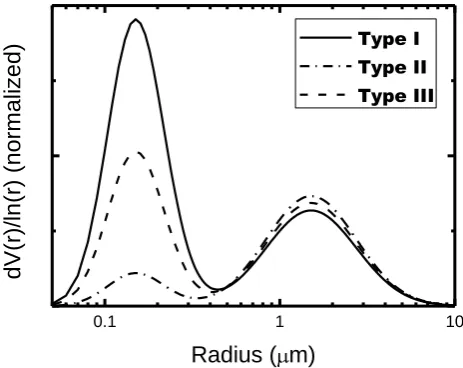
We consider three types of aerosol size distributions for the simulations, which we call type I, type II and type III. These size distributions are used to approximate real aerosol types found in the atmosphere. All types user_fv=0.14 µm, lnσf =0.4,rcv=1.5 µm and lnσc=0.6. These mode radii

and widths are representative of those provided by Dubovik et al. (2002) in the AERONET climatology database and are thus considered to represent a large fraction of naturally oc-curring aerosols. The differences between type I, II and III are the ratio of fine and coarse mode (Vtf/Vtc). Type I yields Vtf/Vtc=2 and represents a distribution with a

3042 D. Pérez-Ramírez et al.: Errors of microphysical particle retrievals from 3β+2αlidar measurements

2003; Müller et al., 2004; Schafer et al., 2008). Type II yields

Vtf/Vtc=0.2 and corresponds to a slight predominance of

the coarse mode over the fine mode. This type is consistent with a mixture of dust/marine aerosol and those of pollution or biomass burning (e.g., Smirnov et al., 2002, 2003; Eck et al., 2005, 2010). Finally, type III yieldsVtf/Vtc=1 and

corresponds to a slight predominance of fine mode over the coarse mode (e.g., Xia et al., 2007; Ogunjobi et al., 2008; Yang and Wenig, 2009; Eck et al., 2009). This type is rep-resentative of predominance of pollution or biomass burning but with considerable influence of dust particles. Figure 1 il-lustrates the three size distributions used. For convenience, the size distributions of Fig. 1 are normalized. Finally, if we were to include a strong predominance of coarse mode (e.g., marine or dust aerosol) in 3β+2αlidar measurements, then the effects of polarization and nonsphericity should be taken into account, and previous work indicates that the use of ker-nel functions for nonspherical particles can improve the re-trievals (Veselovskii et al., 2010). Here, however, our purpose is to calculate sensitivities due to random and systematic un-certainties, so we consider only spherical (Mie) kernels and thus exclude a distribution with a strong predominance of the coarse mode.

The simulation consists in generating the three backscat-tering and two extinction coefficients for the 3β+2α lidar configuration using Mie theory for the three aerosol size dis-tributions: type I, type II and type III. These optical data are generated for six different configurations of aerosol re-fractive indices (mr values of 1.35, 1.45 and 1.55 and mi

either 0.005 or 0.01). From previous studies (Müller et al., 1999b; Veselovskii et al., 2002), error in mr was initially

established as±0.05, while error inmi was approximately

50 %. Moreover, the AERONET network provides refractive indices with very similar errors (Dubovik et al., 2000). Thus, the range of refractive indexes proposed for the size distri-bution is enough to cover most of the values obtained by AERONET (Dubovik et al., 2002).

The regularization inversion is then performed on these data and we obtain the retrieved microphysical parameters

Mret. The next step consists of applying a systematic bias,

denoted as1ε, to one optical datum at a time. The bias varies from−20 to+20 % in eight intervals. For each of these in-duced biases, the inversion is performed and a new size dis-tribution and set of microphysical parameters,Mbias, are then

obtained. The comparisons to be performed are expressed as the percentage difference 100·(Mbias−Mret)/Mret. This

pro-cedure is applied to each of the five optical data used in the 3β+2αlidar configuration.

0.1 1 10

dV(r)/ln

(r) (nor

mal

ize

d)

Radius ( m)

Type I Type II Type III

Figure 1:

Normalized size distributions used for computing the simulated optical data. The ratio

between the volume of fine and coarse mode, V

/V

, is 2 for type I, 0.2 for type II and 1 for type

III.

Fig. 1. Normalized size distributions used for computing the

simu-lated optical data. The ratio between the volume of fine and coarse mode,Vtc/Vtc, is 2 for type I, 0.2 for type II and 1 for type III.

3 Results

3.1 Uncertainties in the retrieval of particle refractive index

The 3β+2αlidar configuration permits the retrieval of parti-cle refractive index, both real (mr)and imaginary (mi)parts

(e.g., Veselovskii et al., 2002), by the use of the regulariza-tion scheme. But the inverse problem of Eq. (1) is underde-termined and, as already stated, constraints are needed to per-mit solutions to be obtained. Particularly, the selection of the range of refractive indices permitted in the retrieval is impor-tant. As commented, we limited the range ofmrto between

1.33 and 1.65 andmifrom 0.0 up to 0.01. These ranges cover

most types of aerosol particles present in the atmosphere, ex-cept for strongly absorbing particles such as black carbon. Moreover, given that the longest wavelength measurement used here is 1064 nm, the technique has reduced sensitivity to the coarse mode of the aerosol distribution. Thus, to sta-bilize the retrievals, the maximum radius of the retrieval in-terval was set to 5 µm. Additionally, the kernel functions for radius below 0.075 are very near to zero, and thus the min-imum radius allowed was set to 0.075 µm. The behavior of the kernel functions versus wavelength can be consulted, for example, in Chapter 11 of Bohren and Huffman (1998).

In the analysis that follows, we do not present results on the refractive index sensitivity analysis. The reason for this is that we found that the retrieval of refractive index is very sensitive to the range of permitted values for the imaginary part of the refractive index. Changing the range of permitted values of the imaginary part can change the retrieved refrac-tive index significantly while not significantly affecting the values of the other retrieved quantities. For example, com-putations allowing mi to range up to 0.1 provide retrieved

values ofmi of approximately 0.03 when the values of mi

of the input size distributions where 0.01 or 0.005. There-fore, keeping in mind that the retrieval is underdetermined, we conclude that we can provide reasonable estimates of the refractive index only with reasonable constraints formi. All

these results just magnify the point that refractive index re-trievals are difficult with the MW lidar technique and that some a priori knowledge of the aerosol absorption is help-ful to constrain the inversion. A more detailed discussion about the limitations of the averaging procedure used here to retrieve accurate values of particle refractive index is in Veselovskii et al. (2013).

3.2 Effects on the retrievals of systematic errors in the optical data

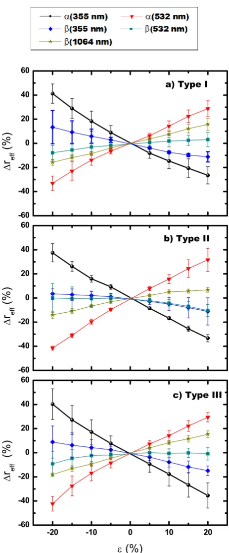
For the scheme described previously, Fig. 2 presents the sen-sitivity analysis for the retrieval of effective radius (reff).

Ev-ery point corresponds to the mean value of the six different combinations of aerosol refractive indices used in generating the set of optical data. The error bars shown are the standard deviations of these mean values. Generally linear patterns are observed for the deviation in the retrieved value ofreff for

differing biases in the input optical data for all of types I, II and III aerosols. As the linear patterns pass through the ori-gin, least-squares fits of the formY =aXwere performed for the points shown in the plot. Given the definition of

1reff=reff,bias−reff,ret, positive slopes indicate higher

val-ues ofreff when the optical data are affected by positive

bi-ases than when they are not affected by bibi-ases, while for neg-ative slopes just the opposite occurs. Moreover, Fig. 2 reveals the same general patterns for all of types I, II and III for each optical channel, with only small changes in the absolute val-ues of the slopes of the linear fits. It is quite apparent that the retrievals are more sensitive to biases in the extinction coeffi-cients. The lowest sensitivities are to biases inβ(355 nm) and

β(532 nm), while for biases inβ(1064 nm), the sensitivity of the retrievals is in between those obtained for extinction and backscattering coefficients at 355 and 532 nm. Figure 2 also reveals that the linear patterns for different optical channels have different signs of the slopes. Considering the parame-ters to which the retrievals are most sensitive, the linear fit of

α(355 nm) gives negative values of slope (a= −1.68±0.12 for type I,a= −1.74±0.03 for type II anda= −1.84±0.04 for type III), while for α(532 nm) the slopes are positive (a=1.51±0.04 for type I,a=1.82±0.09 for type II and

a=1.71±0.10 for type III).

The Ångström law, either for the extinctionα(λ)=kλ−ηα

or for the backscatteringβ(λ)=kλ−ηβ, can be used to help understand the sign of the slopes of Fig. 2. For the wave-lengths used here, the Ångström exponentsηα andηβ

char-acterize the spectral features of aerosol particles and are re-lated to the size of the particles: large values ofηα andηβ

are mainly associated with predominance of fine-mode parti-cles, while low values are associated with a predominance of

Figure

2:

Percentage

deviation

of

the

effective

radius

as

a

function

of

systematic

bias

in

the

optical

data

(

ε

).

a)

Type

I.

b)

Type

II.

C)

Type

III.

-60 -40 -20 0 20 40 60

Δ

r

(%

)

b) Type II

-60 -40 -20 0 20 40 60

Δ

r

(%

)

a) Type I

-20 -10 0 10 20 -60

-40 -20 0 20 40 60

c) Type III

Δ

r

(%)

ε

(%)

Fig. 2. Percentage deviation of the effective radius as a function of

3044 D. Pérez-Ramírez et al.: Errors of microphysical particle retrievals from 3β+2αlidar measurements

coarse mode (e.g., Dubovik et al., 2002). Moreover, many works (e.g., Alados-Arboledas et al., 2003; O’Neill et al., 2005; Veselovskii et al., 2009) have found an inverse rela-tionship between the Ångström exponent for extinction and the effective radius: large values of the Ångström exponent are associated with low values ofreff, while just the

oppo-site occurs for low values of the Ångström exponent. Con-sidering this and given that α(355 nm) is generally larger thanα(532 nm), a positive bias inα(355 nm) increases the spectral difference with α(532 nm) and would increase the value of the Ångström exponent and thus would result in a decrease in the retrieved particle radius. This agrees with the negative slopes ofα(355 nm) observed in Fig. 2. On the other hand, a positive bias inα(532 nm) reduces the spectral difference with α(355 nm) and thus serves to decrease ηα.

Thus, we would expect an increase in the retrieved particle radius, which agrees with the positive slopes observed for

α(532 nm) in Fig. 2. The slopes ofβ(355 nm) andβ(532 nm) possess mostly the same sign as the corresponding extinc-tion coefficient at each wavelength, and similar logic con-cerning the relationship of the Ångström exponent and the particle size given forα(355 nm) andα(532 nm) can be used to explain this behavior as well. Finally, for β(1064 nm) we observe positive slopes (a=0.791±0.008 for type I,

a=0.54±0.07 for type II anda=0.84±0.02 for type III). Positive biases of β(1064 nm) decrease the spectral differ-ence between β(355 nm) and β(532 nm), indicating a de-crease of the Ångström exponent, and thus we would expect an increase in the retrieved particle size, which agrees with the presence of positive slopes in the plot.

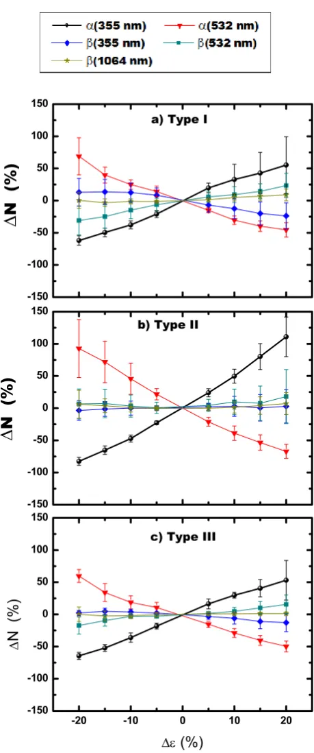
Figure 3 presents the sensitivity analysis for the retrieval of number concentration (N). From Fig. 3 we again gen-erally observe linear patterns of the deviation in retrieved value ofN for differing biases in the input optical data. Lin-ear fits through the origin in the forms Y =aXwere also performed here. Interestingly, the slopes of the linear fits of the extinction coefficients present opposite signs to those determined for the retrieval ofreff, with positive values for α(355 nm) (a=3.09±0.12 for type I,a=4.83±0.22 for type IIa=3.04±0.13 for type III) and negative values for

α(532 nm) (a= −2.78±0.17 for type I,a= −4.09±0.23 for type II anda= −2.61±0.12 for type III). Therefore, we see in the retrieved results, for example, that in order to com-pensate for a radius enhancement due to biased input data, the retrieval tends to decrease number density.

For the sensitivities ofreff andN shown in Figs. 2 and 3,

the absolute values of the slopes atα(355 nm) andα(532 nm) are larger than 1, which indicates that the percentage devia-tions in the retrievedreffandN using biased data are larger

than the percentage bias imposed on the input optical data. Thus, the accuracy ofreff retrievals using 3β+2α lidar is

strongly dependent on the accuracy associated with the ex-tinction coefficients. Other slopes with absolute values less than 1, as for example those obtained forreffas a function of

biases inβ(1064 nm), indicate that while the retrieval is still

Figure 3: Percentage deviation of the number concentration as a function of systematic bias in the 

optical data (ε).  a) Type I. b) Type II. c) Type III.  

-150 -100 -50 0 50 100 150

a) Type I

Δ

N (%)

-150 -100 -50 0 50 100 150

b) Type II

Δ

N (%

)

-20 -10 0 10 20

-150 -100 -50 0 50 100 150

c) Type III

Δ

N

(%)

Δε

(%)

Fig. 3. Percentage deviation of the number concentration as a

func-tion of systematic bias in the optical data (ε). (a) Type I, (b) type II and (c) type III.

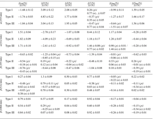
Table 1. Percentage deviations in the aerosol microphysical properties as a function of systematic errors in the optical dataε. Particularly, the slopesaof the linear fitsY =aXare presented, whereXis the systematic bias in the optical data andY is the corresponding deviation in the microphysical properties. All these fits presented linear determination coefficientR2> 0.90. For the cases when there is a difference in slope between positive and negative biases in the input data, the slopes relating to the positive biases are indicated by (p), while those associated with negative biases are indicated by (n).

1reff(%)

1ε(%)

1N (%) 1ε(%)

1S(%) 1ε(%)

1V (%) 1ε(%)

1rfine(%)

1ε(%)

1Vfine(%)

1ε(%)

α

(355

nm)

Type I −1.68±0.12 3.09±0.12 2.08±0.05 0.26 (p)/ −0.99±0.11 1.59±0.05 0.77 (n),±0.07

Type II −1.74±0.03 4.83±0.22 1.77±0.04 −0.37 (p)/ −1.27±0.17 1.66±0.17 0.35 (n)±0.05

Type III −1.84±0.04 3.04±0.13 1.95±0.05 −0.47 (p)/ −0.64 (p)/ 1.56±0.06 0.77 (n)±0.04 −1.51 (n)±0.07

α

(532

nm)

Type I 1.51±0.04 −2.78±0.17 −1.07±0.08 0.44±0.12 1.17±0.04 −0.28±0.05

Type II 1.82±0.09 −4.09±0.23 −0.69±0.03 1.18±0.17 1.28±0.07 −0.44±0.04

Type III 1.71±0.10 −2.61±0.12 −0.92±0.07 1.46±0.08 (p)/ 0.98 (p)±0.01 / −0.20±0.04 0.77 (n)±0.02 1.46 (n)±0.01

β

(355

nm)

Type I −0.63±0.02 −1.25±0.04 (p)/ −0.73±0.04 −1.39±0.04 −0.01 (p)/ −0.62±0.03

−0.85±0.15 (n) −0.06 (n)±0.01

Type II −0.54 (p)/ 0.19 (p)/ −0.22 (p)/ −0.48±0.10 0.33 (p)/ 0.26 (p)/

−0.18 (n)±0.01 0.12 (n)±0.04 −0.04 (n)±0.02 0.06 (n)±0.03 −0.01 (n)±0.01 Type III −0.76 (p)/ −0.44±0.08 −0.47±0.06 −1.04±0.08 0.10±0.01 −0.39 (p)/

−0.43 (n)±0.01 −0.19 (n)±0.01

β

(532

nm)

Type I 0.27±0.04 1.3±0.09 0.50±0.03 0.77±0.05 −0.05 (p)/ 0.22±0.02

−0.22 (n)±0.03

Type II −0.48 (p)/ 0.79±0.11 (p)/ 0.05±0.02 −0.38 (p)/ −0.11±0.02 −0.11 (p)/ 0.02 (n)±0.02 −0.37±0.05 (n) 0.03 (n)±0.03 −0.34 (n)±0.01 Type III −0.03 (p)/ 0.70±0.06 0.30±0.03 0.48±0.07 −0.16±0.01 0.02±0.02

0.38 (n)±0.05

β

(1064

nm)

Type I 0.79±0.01 0.37±0.05 0.17±0.02 0.92±0.04 −0.17±0.01 −0.04±0.01

Type II 0.54±0.07 0.29 (p)/ 0.04±0.02 0.60±0.05 −0.28±0.02 −0.15 (p)/

−0.25 (n)±0.05 −0.34 (n)±0.02

Type III 0.84±0.02 0.07±0.03 0.08±0.02 0.92±0.03 −0.26±0.01 −0.19±0.01

quite sensitive to biases inβ(1064 nm), the deviations in the retrieved parameters is less than the magnitude of the biases. Finally, the slopes ofreffas a function of biases in the input

data forβ(355 nm) andβ(532 nm) are quite small, indicating that biases in these optical parameters have relatively small effects on the retrieval ofreff. However, for the retrieval of

number concentration, the effects of biases in the backscat-tering optical data are not negligible, with absolute values of the slopes of the linear fits between 1.3 and 0.3.

As with the effective radius and number concentration, we have performed the sensitivity analysis for the other micro-physical parameters obtained from the inversion of 3β+2α

lidar data. For these studies, we have also observed generally linear patterns when considering the differences in the re-trieved microphysical parameters as a function of the bias in

the input optical data. Again, the linear patterns pass through the origin, and we therefore assumed least-squares fits of the formY=aX. The results of the linear fits for all the param-eters are summarized in Table 1, including also the slopes obtained forreffandN in Figs. 2 and 3, respectively.

3046 D. Pérez-Ramírez et al.: Errors of microphysical particle retrievals from 3β+2αlidar measurements

of the distribution. From Table 1 we observe that the number concentration is by far the most sensitive parameter to bias in the optical data, particularly to those biases inα(355 nm) and

α(532 nm). Moreover, the sensitivities to biases atβ(355 nm) are generally larger for type I than for type II (absolute values of slopes are larger), with type III being in the middle. This finding can be explained by the fact that, for the same total volume, small particles (which predominate in type I) gener-ally provide larger backscattering of light at the shorter wave-lengths (phase function at 180◦is larger) (e.g., Mischenko et al., 2000; Liou, 2002; Kokhanovsky 2004).

From Table 1 the slopes calculated from the linear fits of surface concentration (S) as a function of biases in the opti-cal data present the same patterns (sign of slopes) between types I, II and III. The difference in the absolute values of slopes between the three types are then associated with the differences in the size distribution and with the changes in the kernel functions. The largest sensitivities ofS are found for biases atα(355 nm) (absolute values of slopes∼2.0). Sen-sitivities to biases atα(532 nm) (absolute values of slopes between 1.07 and 0.69) are also important for type I, II and III, while the sensitivity associated withβ(355 nm) is only remarkable for type I (slope of−0.73±0.04). Sensitivities to biases atβ(532 nm) andβ(1064 nm) are quite low (abso-lute values of slopes below 0.5).

Referring back to Table 1, we observe that the volume concentration (V) is the retrieved integrated parameter least affected by bias in the input optical data, as indicated by the fact that most of the slopes have absolute values below 1.0. However, we found differences among these three dif-ferent aerosol types. For type I aerosols, the retrieval of vol-ume concentration is most sensitive to biases inβ(355 nm) (slope of −1.39), while for type II aerosols, retrievals are most sensitive to deviations in α(532 nm) (slope of 1.18). For type III aerosols the sensitivities to bias in the optical data are important both atβ(355 nm) (slope of−1.04) and at

α(532 nm) (slope up to 1.46). These differences among the aerosol types I, II and III demonstrate the different sensitivi-ties of volume concentration retrievals when the aerosol size distribution possesses different weights of fine and coarse mode.

As the regularization scheme used here computes the size distribution using the range of permitted radii of 0.075–5 µm, the fine-mode part of the distribution (but not the coarse mode) is completely covered by this inversion window, and thus we study fine-mode volume radius (rfine) and fine-mode

volume concentration (Vfine). Table 1 also shows the

sensi-tivities of these two parameters to biases in the input opti-cal data. From the slopes of the linear fits reported forrfine,

biases inα(355 nm) andα(532 nm) produce significant de-viations in the retrieval, with absolute values of the slopes approximately between 1.0 and 1.5, while the deviations in the retrievals created by biases in other optical parameters are almost negligible. This result would imply that accu-rate retrievals ofrfine can tolerate rather large errors in the

backscatter data but not in the extinction data. The sign of the slopes ofrfineas a function ofα(355 nm) andα(532 nm) can

be explained by the same reasoning given before for the ef-fective radius: as extinction at 355 nm increases, it makes the retrieved particle radius decrease. But asα(532 nm) increases the retrieved particle radius increases. On the other hand, for theVfine, the largest sensitivities in the retrieval are found to

systematic biases atα(355 nm), with slopes of 1.59±0.05, 1.66±0.17 and 1.56±0.06 for types I, II and III, respec-tively. For the other optical parameters, absolute values of the slopes are below 0.5 (exceptβ(1064 nm) for type I with slope of 0.62±0.03). These dependencies of the sensitivities ofrfineandVfine to biased input data are associated with the

different dependencies of the kernel functions on wavelength and particle radius (e.g., Chapter 11 of Bohren and Huffman, 1998).

At this point we would like to mention that our simulations (graphs not shown for brevity) showed some departures from the linearity shown in Figs. 2 and 3 and Table 1 for systematic errors larger than approximately±30 %, mainly when the ab-solute values of the slopes are larger than 1. We take this to be an indication that biases of approximately±30 % and larger can cause the regularization routine to choose a different so-lution space than the original retrieval based on data with no errors. On the other hand, up to errors of±20 %, we find that the same minimum in the solution space is generally found by the routine, so the linear behavior seen in Figs. 2 and 3 is taken to be a characteristic of a stable system that is displaced from its minimum point. Therefore, we selected a threshold value of±20 % where these results are applicable and stress that larger errors in the input data can cause significant and unpredictable deviations in the retrieved results.

Finally, we remark that the values given in Table 1 are av-eraged for the particular size distributions used here. More simulations performed (graphs not shown for brevity) chang-ing the fine-mode radius between 0.08 and 0.20 µm, for aerosol types I, II and III, revealed the same average lin-ear patterns as those shown in Figs. 2 and 3 and in Table 1. The only differences observed were in the absolute values of the slopes with differences within 10 %. On the other hand, no important departures from the linearity observed in Ta-ble 1 were found by changing the widths of the fine mode. Changes in the coarse mode were not tested because of the difficulty to assess retrievals of the coarse mode with the methodology used here.

3.2.1 Effects of the constraints used in the retrievals on the sensitivity test results

The sensitivity tests applied to the different sets of data have shown linear dependencies. The data presented in Table 1 of the linear fits allow for the computation of the deviations in-duced in retrieved quantities due to biases in the input data in an easy and straightforward way. But the generality of the results for different constraints in the inversion code needs

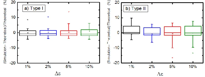
Figure 4:

For the effective radius, Box-Whisker diagrams of the differences between the

theoretical deviations computed with the slopes of table 1 and the simulated deviations

.

At least

two optical channels have been simultaneously perturbed by biases of the same magnitude

although different combinations of over/under estimations are allowed. In these box diagrams the

mean is represented by an open square. The line segment in the box is the median. The top limit

represents the 75

percentile (P75) and the bottom limit the 25

percentile (P25). The box bars

are related to the 1

(P1) and 99

(P99) percentiles, and the crosses represent the maximum and

minimum values respectively. We used biases in the optical data of 1% (black diagrams), 2%

(blue diagrams), 5% (red diagrams) and 10% (green diagrams).

Fig. 4. For the effective radius, box-and-whisker diagrams of the differences between the theoretical deviations computed with the slopes

of Table 1 and the simulated deviations. At least two optical channels have been simultaneously perturbed by biases of the same magnitude although different combinations of over/underestimations are allowed. In these box diagrams the mean is represented by an open square. The line segment in the box is the median. The top limit represents the 75th percentile (P75) and the bottom limit the 25th percentile (P25). The box bars are related to the 1st (P1) and 99th (P99) percentiles, and the crosses represent the maximum and minimum values, respectively. We used biases in the optical data of 1 (black diagrams), 2 (blue diagrams), 5 (red diagrams) and 10 % (green diagrams).

to be examined. For example, the results presented in Ta-ble 1 have been based on a maximum radius in the inver-sion (rmax)of 5 µm. Although for the aerosol size

distribu-tions studied here thisrmaxmakes the computation more

ef-ficient, the selection ofrmaxdepends on the user and becomes

a constraint in the inversion procedure. Thus, we performed more simulations withrmaxincreased to a value of 10 µm to

study the influence of this change in constraint on the re-trieved results. Another constraint in the inversion that must be checked is the maximum value allowed formi. We

re-peated the simulations allowingmito range up to 0.1

(con-sistent with a very absorbing aerosol like black carbon). The results of these studies were compared with a baseline re-trieval obtained withrmax=5 µm and with maximum value

ofmiof 0.01. To compute the baseline microphysical

param-eters, no induced systematic errors were included. We also computed the retrievals using the new constraints and intro-ducing systematic errors in the optical data as done before.

The new simulations performed after changing the con-straints for rmax and maximum mi also reveal linear

pat-terns (graphs not shown for brevity). However, these linear patterns do not pass through the origin, implying that there are generally shifts in the retrieved values of the various pa-rameters due to these changes in constraints. The analysis reveals, though, that the signs of the slopes of the linear fits remain the same and that very similar deviations in the retrieved quantities are computed using the linear fits per-formed. Therefore, while the selection of exact value of the constraints forrmaxandmican change the mean values of the

different parameters, the sensitivity to induced biases in the input optical data is generally unchanged by these changes in constraints.

3.2.2 Additive properties of the effects of systematic errors in the optical data

Thus far, the sensitivity tests that have been performed were based on perturbing a single optical input at a time. But in a real instrument, it is quite possible that two or more input data might be influenced by biases simultaneously. There-fore, we need to study the effects of the presence of multiple simultaneous biases in the input data since the existence of such biases would presumably not be known in a real ap-plication. In other words, we wish to determine if the pre-ceding results based on perturbing a single optical input at a time can be generalized to predict the effects of multiple input data being simultaneously biased. In particular, we will now test if, when multiple inputs are simultaneously biased, the results from Table 1 can be used to calculate deviations that can simply be added to determine the total bias. In other words, we now will test whether the results in Table 1 can be considered additive.

3048 D. Pérez-Ramírez et al.: Errors of microphysical particle retrievals from 3β+2αlidar measurements

the differences in the microphysical properties based on the slopes given in Table 1 and those actually retrieved running the code with the new biased optical data and then charac-terized the differences. Using this procedure, we generated for each absolute value of bias a statistical data set that in-cludes many different configurations of the different optical channels. Those data sets are analyzed using Bow–Whisker diagrams as shown in Fig. 4 for the effective radius.

In these box diagrams the mean is represented by an open square. The line segment in the box is the median. The top limit represents the 75th percentile (P75) and the bottom limit the 25th percentile (P25). The box bars are related to the 1st (P1) and 99th (P99) percentiles, and the crosses repre-sent the maximum and minimum values, respectively. From Fig. 4, for biases of 1, 2, 5 and 10 %, mean values of the differences in the effective radius are very small: 0.03, 0.34, 0.41 and 1.01 % for type I (Fig. 3a) and−0.62,−0.91,−0.49 and−0.18 % for type II (Fig. 3b). Values larger than the 25th percentiles (P25) and lower than the 75 % percentiles (P75) are found for the ranges from−1.8 to 1.3 % (type I) and from

−0.6 to 4.4 % (type II). Only two outliers are found with rel-ative differences greater than 100 %. The latter occur when all the optical channels exceptβ(355 nm) are either overes-timated or underesoveres-timated. But for these particular cases the baseline deviations are 0.009 or−0.009 %, while the simu-lated ones are 0.557 and−0.557 %, respectively. These small errors are within the uncertainties associated with the regu-larization method, and thus these large relative differences are a mathematical artifact created by dividing by small num-bers. Tests have also been performed for the other microphys-ical parameters, and we also found an additive property in the deviations predicted by the results shown in Table 1. Further-more, very similar additive properties were found for aerosol type III (graph not shown for brevity). Therefore, for the bi-modal size distributions used here that cover most of those size distributions obtained by AERONET, we conclude that the results of Table 1 can be reliably used to calculate the deviations in retrieved quantities due to multiple simultane-ously biased input data.

We take this result to be an indication that, as mentioned earlier, the solutions found by the inversion technique gener-ally define a local minimum in the multidimensional solution space (e.g., see Fig. 1 in both Veselovskii et al., 2002, 2012). The linear behavior of the deviations in the retrieval due to small changes in the input parameters is a characteristic of displacements from this minimum location. Multiple simul-taneous displacements tend also to display this linear behav-ior. The results here indicate therefore, for biases in the input data of up to approximately 20 %, whether for a single chan-nel or multiple ones simultaneously, that the solution space possesses an average linear property and an additive behav-ior can be assumed. For larger biases in the optical data (e.g.,

±30 %) the additive property is not assured, as under these circumstances different minima in the solution space may be found by the regularization algorithm.

3.3 Application to the sensitivity of retrievals to the presence of random errors in the optical data

Up to this point, we have concerned ourselves only with the effects of systematic biases in the input optical data on the retrieved quantities. But in lidar systems, random errors are also present due just to the measurement process itself. Any specific set of 3β+2αdata affected by random errors can be considered as a set of biased measurements where the indi-vidual biases for each of the data follow a normal distribu-tion. Given the additive property of the systematic errors that we have shown, we can assess the effects of random errors in the optical data by generating random biases in the optical data and computing their deviations in the microphysical pa-rameters from the values given in Table 1. The sensitivities of the regularization technique to those random errors com-puted using the procedure just outlined will be compared with previously published ones (e.g., Müller et al., 1999a, b; Veselovskii et al., 2002, 2004).

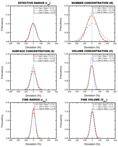
To assess the sensitivity of the retrievals to random errors, we use the additive properties of the systematic biases just described. The procedure used consists of generating ran-dom numbers distributed in a Gaussian way centered at zero with width according to the value of the random error to study. These random errors are applied to each optical chan-nel of the 3β+2αconfiguration. This procedure was repeated 50 000 times for each parameter studied. Also, the initiation of the random number generation is different for each chan-nel in order to avoid the situation where all the random num-bers are the same in every channel. Finally, we introduced this random number for every optical datum and computed the corresponding error in the retrieved microphysical pa-rameter using the slopes provided in Table 1. For every set of 3β+2αvalues, the final error obtained in the microphysical parameter is the sum of the error obtained for each channel. The study of the frequency distributions of the final errors for this large number of simulations yields the effects of ran-dom errors. If the frequency distribution is a normal one, the standard deviation (full width at half maximum) provides the final error in the microphysical parameter. Moreover, if the normal distribution is not centered at zero it demonstrates an interesting property: that the presence of systematic errors in the retrieved microphysical property can be induced by ran-dom errors in the input optical data. As an illustration, Fig. 5 shows the frequency distribution of the differences in the mi-crophysical parameters studied here, for all aerosol size dis-tributions type I, II and III, where 15 % random error is as-sumed in all the optical data. Those differences associated with the effects of random errors are in percentages and de-noted as “deviation” in thexaxis of the histograms.

From Fig. 5 we observe that the frequency distributions possess the expected Gaussian shape for all the microphysi-cal parameters. Most of the frequency distributions are cen-tered essentially at zero, although some significant depar-tures from this value are observed. The percentage changes

Figure 5:

Frequency distributions of the different microphysical parameters for 15% random

errors in the optical data using 50000 random samplings of the systematic error sensitivities

shown in Table 1. The ‘x’ axis represents the difference between microphysical parameters with

no errors in the input optical data and those affected by random errors in the optical data.

Random errors were simulated by a normal distribution centred at zero and with standard

deviation of 15%. The random number generator is initialized at different values for each of the

5 optical data used in the 3β + 2α lidar configuration. The mean value of the deviation between

the microphysical parameter affected by random error and that unaffected by random error is

included in the legend.

-300 -200 -100 0 100 200 300 0.00

0.05 0.10 0.15 0.20

Frecue

ncy

Deviation (%)

Type I, Mean = -0.1 % Type II, Mean = -5.3 % Type III, Mean = -4.5 % EFFECTIVE RADIUS (r_eff)

-300 -200 -100 0 100 200 300 0.00

0.05 0.10 0.15 0.20

Type I, Mean = -0.9 % Type II, Mean = 11.1 % Type III, Mean = 0.4 %

Frecue

ncy

Deviation (%)

NUMBER CONCENTRATION (N)

-300 -200 -100 0 100 200 300 0.00

0.05 0.10 0.15 0.20

Type I, Mean = 0.3 % Type II, Mean = -0.9 % Type III, Mean = 0.2 %

Frecue

ncy

Deviation (%)

SURFACE CONCENTRATION (S)

-300 -200 -100 0 100 200 300 0.00

0.05 0.10 0.15 0.20

Type I, Mean = -2.8 % Type II, Mean = -6.7 % Type III, Mean = -3.1 %

Frecue

ncy

Deviation (%)

VOLUME CONCENTRATION (V)

-300 -200 -100 0 100 200 300 0.00

0.05 0.10 0.15 0.20

Type I, Mean = 1.2 % Type II, Mean = 1.4 % Type III, Mean = 2.3 %

Frecue

ncy

Deviation (%) FINE RADIUS (r_fine)

-300 -200 -100 0 100 200 300 0.00

0.05 0.10 0.15 0.20

Type I, Mean = 0.2 % Type II, Mean = 4.2 % Type III, Mean = -1.1 %

Frecue

ncy

Deviation (%) FINE VOLUME (V_fine)

Fig. 5. Frequency distributions of the different microphysical parameters for 15 % random errors in the optical data using 50 000 random

samplings of the systematic error sensitivities shown in Table 1. Thex axis represents the difference between microphysical parameters with no errors in the input optical data and those affected by random errors in the optical data. Random errors were simulated by a normal distribution centered at zero and with a standard deviation of 15 %. The random number generator is initialized at different values for each of the 5 optical data used in the 3β+2αlidar configuration. The mean value of the deviation between the microphysical parameter affected by random error and that unaffected by random error is included in the legend.

in the mean values of the distributions are shown in the leg-end. A shift in the mean value due to the presence of random error is explained by the different linear tendency for posi-tive and negaposi-tive biases for some input optical data, as dis-cussed earlier to respect Table 1. For example, such depar-tures from zero are observed for retrievals ofreff,N andV

3050 D. Pérez-Ramírez et al.: Errors of microphysical particle retrievals from 3β+2αlidar measurements

Table 2. Standard deviations of the frequency distributions of the deviation induced in the microphysical parameters due to random errors in

the optical data.

reff N S V rfine Vfine

Random Type Type Type Type Type Type Type Type Type Type Type Type Type Type Type Type Type Type

Errors (%) I II III I II III I II III I II III I II III I II III

5 12.5 13.1 13.7 22.5 31.8 20.5 12.5 9.5 11.2 9.8 7.2 9.5 7.7 9.2 8.4 8.7 8.8 8.1

10 24.9 26.2 27.2 45.0 63.6 40.8 25.1 19.1 22.3 19.6 14.4 19.0 15.5 18.4 16.8 17.4 17.6 16.1

15 37.2 39.2 40.8 67.6 95.2 61.4 37.7 28.5 33.4 29.5 21.5 28.5 23.3 27.6 25.3 26.1 26.3 24.1

20 50.0 52.6 54.8 90.1 127.3 82.1 50.2 38.2 44.6 39.3 28.8 38.0 31.1 36.9 33.8 34.9 35.2 32.2

10∗ ₂₅∗ ₇₀∗ ₂₅∗ ₂₅∗ _{– –}

∗_{From the previous work of Muller et al. (1999a, b) and Veselovskii et al. (2002, 2004).}

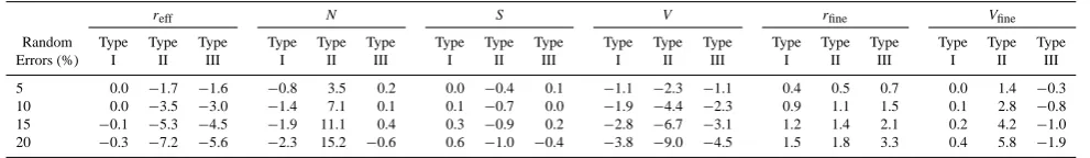
Table 3. Mean of the differences (in percentages) in the retrieved microphysical parameters due to varying amounts of random error in the

optical data.

reff N S V rfine Vfine

Random Type Type Type Type Type Type Type Type Type Type Type Type Type Type Type Type Type Type

Errors (%) I II III I II III I II III I II III I II III I II III

5 0.0 −1.7 −1.6 −0.8 3.5 0.2 0.0 −0.4 0.1 −1.1 −2.3 −1.1 0.4 0.5 0.7 0.0 1.4 −0.3

10 0.0 −3.5 −3.0 −1.4 7.1 0.1 0.1 −0.7 0.0 −1.9 −4.4 −2.3 0.9 1.1 1.5 0.1 2.8 −0.8

15 −0.1 −5.3 −4.5 −1.9 11.1 0.4 0.3 −0.9 0.2 −2.8 −6.7 −3.1 1.2 1.4 2.1 0.2 4.2 −1.0

20 −0.3 −7.2 −5.6 −2.3 15.2 −0.6 0.6 −1.0 −0.4 −3.8 −9.0 −4.5 1.5 1.8 3.3 0.4 5.8 −1.9

clearly thatV,rfineandVfine exhibit the smallest sensitivity

to the imposed 15 % random errors with a 1-sigma spread in the result of approximately 25 %. The effective radius and surface concentration results show moderate sensitivity with 1-sigma values of∼30–40 %, while the retrieval of number concentration has the highest sensitivity, with 1-sigma val-ues of 67.6 % for type I, 95.2 % for type II and 61.4 % for type III. As expected, these sensitivities to random error track the results of the sensitivities to systematic errors, where the most sensitive parameter was also found to be number con-centration and the least sensitive were volume concon-centration, fine-mode radius and fine-mode volume concentration.

Using the same procedure as for 15 % random error, Ta-ble 2 reports the FWHM – or standard deviations – of normal distributions obtained for other magnitudes of random errors in the optical data ranging from 5 to 20 %. We observe, as expected from the linear functions involved, that increasing the random uncertainty increases the deviations found in a linear fashion. Moreover, it is observed again that the largest sensitivities are forN, while the lowest are forV,rfine and Vfine. In the same way, Table 3 reports the means of the

de-viation of every microphysical property for varying amounts of random uncertainty in the input data. As mentioned above, the departures of these deviations from zero indicate that ran-dom uncertainties in the input optical data can induce vary-ing amounts of systematic bias in the retrieved properties. This effect is found more with the type II aerosols that pos-sess a higher fraction of larger particles. Such a population is more likely to have different slopes in Table 1 due to positive and negative biases in the input optical data because of the reduced sensitivity of the MW technique to larger particles. It is this reduced sensitivity to larger particles that, in gen-eral, explains the shifting of the mean values in the retrieved

distributions due to varying amounts of random error in the input data.

Müller et al. (1999a, b) and Veselovskii et al. (2002, 2004) studied 10 % random uncertainties in the optical data in the 3β+2αlidar configurations by introducing random errors in the optical data and running the regularization code repeat-edly. These studies reported that the retrieved uncertainties were on the order of 25 % forreff,V andS, 30 % forrmean

and 70 % forN. These values are quite similar to those re-ported in Table 2 for our computations of 10 % random er-rors. No evaluations forrfineandVfinewere done in the

stud-ies of Müller et al. (1999a, b) and Veselovskii et al. (2002, 2004). The method shown here for assessing the sensitivity of retrievals to random errors is generally consistent with these earlier results but permits the influence of varying amounts of random error to be studied. It also permits the influence of random errors in different input optical channels to be quan-tified. We will now apply this capability to the problem of instrument specification.

Application to instrument specification

The upcoming spaceborne Decadal Survey ACE (Aerosol-Cloud-Ecosystems) mission of NASA (http://dsm.gsfc.nasa. gov/ace/) specifies a high-spectral-resolution lidar as a core instrument to measure vertical profiles of aerosol extinction and backscattering worldwide. These profiles will be used to derive vertically resolved aerosol microphysical properties such as effective radius, number concentration or complex refractive index. The system is anticipated to use the 3β+2α

configuration and the regularization technique that has been studied here. The first reports (http://dsm.gsfc.nasa.gov/ace/) call for an accuracy of ±15 % for all backscattering and

extinction coefficients, and thus the results presented here can be used to infer the anticipated uncertainties in the mi-crophysical properties retrieved using the regularization tech-nique on these 3β+2αspaceborne data when all input data possess 15 % uncertainties. However, the results already pre-sented clearly indicate that, for most quantities, it is uncer-tainties in the extinction coefficients that need to be con-strained more carefully than those in the backscattering data. Volume concentration is an interesting exception to this state-ment whereβ(355 nm) for type I aerosols is the optical pa-rameter requiring the smallest uncertainty budget to help re-duce the uncertainties in retrievals. In this way, the results obtained here can serve as a guide to hardware designers of multiwavelength lidar instruments in the sense that if trade-offs need to be made between the performance of one op-tical channel versus another, the relative sensitivities shown in Table 1 can be used to assess which channels would ben-efit most from decreased uncertainty in the measurements. Another application of the sensitivities derived here is to al-gorithm development. Alal-gorithms can introduce systematic uncertainties in the optical data such as through an incor-rect assumption of an aerosol-free region, an assumption of the extinction to backscatter ratio or the use of an estimated molecular profile. The results presented here can be used to assess the tolerance for both random and systematic errors in the input optical data due both to instrumentation and to algo-rithms once uncertainty requirements in the retrieved quanti-ties are established.

4 Summary and conclusions

We have presented the results of a study of the sensitivity of the retrievals of aerosol physical parameters using the reg-ularization technique to systematic and random uncertain-ties in the input optical data. We have focused our study on the set of data consisting of three backscattering coefficients (β)at 355, 532 and 1064 nm and two extinction coefficients (α)at 355 and 532 nm (3β+2αconfiguration). These data can be obtained by a lidar system that uses a Nd:YAG laser and combines backscatter with Raman or HSRL channels. Simulations have been done for different bimodal aerosol size distributions that are representative of AERONET cli-matologies. The values used for aerosol refractive indexes, as well as mode radius and widths, were selected as representa-tive of those climatologies as well. The selected aerosol bi-modal size distributions include one with fine-mode predom-inance (type I), another with predompredom-inance of coarse mode but with significant presence of fine mode (type II) and an-other with predominance of fine mode but with significant presence of coarse mode (type III). Optical data consistent with these bimodal size distributions were generated using Mie theory. Retrievals were performed using these baseline optical data. The optical data were then perturbed by system-atic biases in the range±20 % to study the effects of biases

on the retrieved parameters. This threshold value of±20 % is enough for many practical lidar applications. As the prob-lem of the inversion of microphysical properties is underde-termined, constraints are needed that, in principle, can influ-ence the values retrieved by the algorithm. Particularly, we have found that the range of radius and refractive index used in the inversion did not have a large influence on the sen-sitivities of the different microphysical particles. However, our results showed that the maximum value ofmiallowed in

the retrieval had a significant influence on the value of the refractive index retrieved, supporting earlier results that in-dicate significant uncertainties in the retrieval of refractive index using the 3β+2αMW lidar technique studied here.

The microphysical parameters studied included effective radius (reff)and volume (V) as well as number (N) and

sur-face (S) concentration. Also, as the inversion window ranged from 0.075 to 5 µm, we were able to study the fine mode of the aerosol size distribution (0.075–0.5 µm) separately, and thus we have also presented the results for both fine-mode radius (rfine)and volume (Vfine). From these sensitivity tests,

the percentage deviations of the microphysical parameters as a function of biases in the optical data presented linear pat-terns. Generally, these linear patterns presented the same sign of slopes for aerosol type I, II and III and the largest sensi-tivities were observed for biases in the extinction coefficients

α(355 nm) andα(532 nm). Moreover, the largest sensitivities were found forN, while the least affected parameters were

V,rfineandVfine.

An important result is that we have found an additive prop-erty for the deviations induced by the biases in the optical data. This implies that if, for example, several optical data are simultaneously affected by systematic errors, the total devi-ation in the retrieved quantity can be well approximated by the sum of those deviations computed when each optical in-put was biased separately. From this additive property, we have been able to compute the effects of random errors in the optical data. Moreover, we have found some systematic dif-ferences in the mean retrieved microphysical properties when the retrievals are affected by random errors in the input opti-cal data. The presence of these systematic differences is asso-ciated with the different behavior (although with linear pat-terns) between positive and negative biases in the input opti-cal data, and is due to a reduced sensitivity of the retrieval to the coarse part of the size distribution.

3052 D. Pérez-Ramírez et al.: Errors of microphysical particle retrievals from 3β+2αlidar measurements

a wide range of lidar applications, and thus can be used to es-tablish acceptable error budgets in optical data if maximum permissible errors in the retrieved quantities can be estab-lished. Therefore, the values given here for the sensitivities of the microphysical properties to systematic errors in the opti-cal data can be useful for many lidar applications. For exam-ple, for the Decadal Survey ACE mission, a multiwavelength lidar is planned. Among their measurement requirements is that the accuracy of the optical data be±15 %. If these un-certainties are taken to be all random, we were able to use the results here to estimate that this implies an uncertainty in the retrieved microphysical properties by the regularization technique of∼40 % for reff,∼85 % forN,∼25 % for S, ∼20 % forV, and 16 % forrfineandVfine, respectively. The

results also permit assessing the deviations in the retrievals if the biases in the optical data are systematic and exist in only one or more channels. In this way, trade-off decisions can be made between the retrieval requirements and the hardware configuration of a lidar system taking into account the differ-ent sensitivities of the retrievals to biases in the optical data of different channels. We hope these results aid the future de-sign of multiwavelength lidar systems intended for retrieval of aerosol microphysical properties.

Acknowledgements. This work was supported by the NASA/Goddard Space Flight Center, the Spanish Ministry of Science and Technology through projects CGL2010-18782 and CSD2007-00067, the Andalusian Regional Government through projects P10-RNM-6299 and P08-RNM-3568, the EU through ACTRIS project (EU INFRA-2010-1.1.16-262254) and the Post-doctoral Program of the University of Granada. We also express our gratitude to the anonymous referees for their suggestions to improve this work.

Edited by: V. Amiridis

References

Alados-Arboledas, L., Lyamani, H., and Olmo, F. J.: Aerosol size properties at Armilla, Granada (Spain), Q. J. Roy. Meteorol. Soc., 129, 1395–1413, doi:10.1256/qj.01.207, 2003.

Alados-Arboledas, L., Müller, D., Guerrero-Rascado, J. L., Navas-Guzmán, F., Pérez-Ramírez, D., and Olmo, F. J.: Optical and microphysical properties of fresh biomass burning aerosol re-trieved by Raman lidar, and star-and sun-photometry, Geophys. Res. Lett., 38, L01807, doi:10.1029/2010gl045999, 2011. Ansmann, A., Riebesell, M., Wandinger, U., Weitkamp, C., Voss,

E., Lahmann, W., and Michaelis, W.: Combined Raman elastic-backscatter LIDAR vertical profiling of moisture, aerosol extinc-tion, backscatter and LIDAR ratio, Appl. Phys. B, 55, 18–28, 1992.

Balis, D., Giannakaki, E., Müller, D., Amiridis, V., Kelektsoglou, K., Rapsomanikis, S., and Bais, A.: Estimation of the micro-physical aerosol properties over Thessaloniki, Greece, during the SCOUT-O3 campaign with the synergy of Raman lidar

and Sun photometer data, J. Geophys. Res., 115, D08202, doi:10.1029/2009JD013088, 2010.

Böckmann, C., Miranova, I., Müller, D., Scheidenbach, L., and Nessler, R.: Mycrophysical aerosol parameters from multiwave-length lidar, J. Opt. Soc. Am. A, 22, 518–528, 2005.

Bohren, C. F. and Huffman, D. R.: Absorption and scattering of light by small particles, John Wiley & Sons, Inc., 1998. Dubovik, O., Holben, B., Eck, T. F., Smirnov, A., Kaufman, Y. J.,

King, M. D., Tanre, D., and Slutsker, I.: Variability of absorption and optical properties of key aerosol types observed in world-wide locations, J. Atmos. Sci., 59, 590–608, 2002.

Eck, T. F., Holben, B. N., Ward, D. E., Mukelabai, M. M., Dubovik, O., Smirnov, A., Schafer, J. S., Hsu, N. C., Piketh, S. J., Queface, A., Le Roux, J., Swap, R. J., and Slutsker, I.: Variability of biomass burning aerosol optical characteristics in southern Africa during the SAFARI2000 dry season cam-paign and a comparison of single scattering albedo estimates from radiometric measurements, J. Geophys. Res., 108, 8477, doi:10.1029/2002JD002321, 2003.

Eck, T. F., Holben, B. N., Dubovik, O., Smirnov, A., Goloub, P., Chen, H. B., Chatenet, B., Gomes, L., Zhang, X. Y., Tsay, S. C., Ji, Q., Giles, D., and Slutsker, I.: Columnar aerosol proper-ties at AERONET sites in central eastern Asia and aerosol trans-port to the tropical mid-Pacific, J. Geophys. Res., 110, D06202, doi:10.1029/2004JD005274, 2005.

Eck, T. F., Holben, B. N., Reid, J. S., Sinyuk, A., Hyer, E. J., O’Neill, N. T., Shaw, G. E., Vande Castle, J. R., Chapin, F. S., Dubovik, O., Smirnov, A., Vermote, E., Schafer, J. S., Giles, D., Slutsker, I., Sorokine, M., and Newcomb, W. W.: Optical properties of boreal region biomass burning aerosols in central Alaska and seasonal variation of aerosol optical depth at an Arctic coastal site, J. Geophys. Res., 114, D11201, doi:10.1029/2008JD010870, 2009.

Eck, T. F., Holben, B. N., Sinyuk, A., Pinker, R. T., Goloub, P., Chen, H., Chatenet, B., Li, Zi., Singh, R. P., Tripathi, S. N., Reid, J. S., Giles, D. M., Dubovik, O., O’Neill, N. T., Smirnov, A., Wang, P., and Xia, X.: Climatological aspects of the opti-cal properties of fine/coarse mode aerosol mixtures, J. Geophys. Res., 115, D19205, doi:10.1029/2010JD014002, 2010.

Forster, P., Ramaswamy, V., Artaxo, P., Berntsen, T., Betts, R., Fa-hey, D. W., Haywood, J., Lean, J., Lowe, D. C., Myhre, G., Nganga, J., Prinn, R., Raga, G., Schulz, M., and Dorland, R. V.: Changes in Atmospheric Constituents and in Radiative Forc-ing, Climate Change 2007: The Physical Science Basis, In: Con-tribution of Working Group I to the Fourth Assessment Report of the Intergovernmental Panel on Climate Change, edited by: Solomon, S., Qin, D., Manning, M., Chen, Z., Marquis, M., Av-eryt, K. B., Tignor, M., and Miller, H. L., 2007.

Grund, C. J. and Eloranta, E. W.: University-of-Wisconsin High Spectral Resolution Lidar, Opt. Eng., 30, 6–12, 1991.

Haywood, J. M. and Boucher, O.: Estimates of the direct and in-direct radiative forcing due to tropospheric aerosols: A review, Rev. Geophys., 38, 513–543, 2000.

Heintzenberg, J., Muller, H., Quenzel, H., and Thomalla, E.: In-formation content of optical data with respect to aerosol proper-ties: numerical studies with a randomized minimization-search-technique inversion algorithm, Appl. Optics, 20, 1308–1315, 1981.

Holben, B. N., Eck, T. F., Slutsker, I., Tanré, D., Buis, J. P., Set-zer, A., Vermote, E., Reagan, J. A., Kaufman, Y. J., Nakajima, T., Lavenu, F., Jankowiak, I., and Smirnov, A.: AERONET – A Federated instrument network and data archive for aerosol char-acterization, Remote Sens. Environ., 66, 1–16, 1998.

Horvath, H., Gunter, R. L., and Wilkison, S. W.: Determintation of the coarse mode of the atmospheric aerosol using data from a forward-scattering spectrometer probe, Aerosol Sci. Technol., 12, 964–980, 1990.

Kaufman, Y. J., Wald, A. E., Remer, L. A., Gao, B. C., Li, R. R., and Flynn, L.: The MODIS 2.1- µm channel – Correlation with visible reflectance for use in remote sensing of aerosol, IEEE T. Geosci. Remote, 35, 1286–1298, 1997.

Liou, K. N.: An introduction to atmospheric radiation, International Geophysics Series, Vol. 84, edited by: Dmowska, R., Holtan, J. T., and Rossby, H. T., 2002.

Kokhanovsky, A. A.: Light scattering media optics, Problems and solutions, Springer-Verlag, 2004.

Mischenko, M. I., Hovenir, J. W., and Travis, L.: Light scattering by nonspherical particles. San Diego, Academic Press, 690 pp., 2000.

Müller, D., Wandinger, U., and Ansmann, A.: Mycrophysical parti-cle parameters from extinction and backscatter lidar data by in-version with regularization: theory, Appl. Optics, 38, 2346–2357, 1999a.

Müller, D., Wandinger, U., and Ansmann, A.: Mycrophysical parti-cle parameters from extinction and backscatter lidar data by in-version with regularization: simulation, Appl. Optics, 38, 2358– 2368, 1999b.

Müller, D., Wagner, F., Wandinger, U., Ansmann, A., Wendisch, M., Althausen, D., and von Hoyningen-Huene, W.: Mycrophysi-cal particle parameters from extinction and backscatter lidar data by inversion with regularization: experiment, Appl. Optics, 39, 1879–1892, 2000.

Müller, D., Wandinger, U., Althausen, D., and Fiebig, M.: Compre-hensive particle characterizations from three-wavelength Raman-lidar observations: case study, Appl. Optics, 40, 4863–4869, 2001.

Müller, D., Mattis, I., Ansmann, A., Wehner, B., Althausen, D., Wandinger, U., and Dubovik, O.: Closure study on optical and microphysical properties of a mixed urban and Arctic haze air mass observed with Raman lidar and Sun photometer, J. Geo-phys. Res., 109, D13206, doi:10.1029/2003JD004200, 2004. Müller, D., Mattis, I., Wandinger, U., Ansmann, A., Althausen, D.,

and Stohl, A.: Raman lidar observations of aged Siberian and Canadian forest fire smoke in the free troposphere over Ger-many in 2003: Microphysical particle characterization, J. Geo-phys. Res., 110, D17201, doi:10.1029/2004JD005756, 2005. Müller, D., Kolgotin, A., Mattis, I., Petzold, A., and Stohl, A.:

Verti-cal profiles of microphysiVerti-cal particle properties derived from in-version with two-dimensional regularization of multiwavelength Raman lidar data: experiment, Appl. Optics, 50, 2069–2079, 2011.

Navas-Guzmán, F., Müller, D., Bravo-Aranda, J. A., Guerrero-Rascado, J. L., Granados-Muñoz, M. J., Pérez-Ramírez, D., Olmo, F. J., and Alados-Arboledas, L.: Eruption of the Eyjaf-jallajokull volcano in spring 2010: Multiwalength Raman lidar measurements of sulphate particles in the lower troposphere, J. Geophys. Res., 118, 1–10, doi:10.1002/jgrd.50116, 2013.

Noh, Y. M., Müller, D., Shin, D. H., Lee, H., Jung, J. S., Lee, K. H., Cribb, M., Li, Z., and Kim, Y. J.: Optical and microphysical prop-erties of severe haze a