www.drink-water-eng-sci.net/1/27/2008/
©Author(s) 2008. This work is distributed under the Creative Commons Attribution 3.0 License.
Engineering and Science
Importance of demand modelling in network water
quality models: a review
E. J. M. Blokker1,2, J. H. G. Vreeburg1,2, S. G. Buchberger3, and J. C. van Dijk3
1Kiwa Water Research Groningenhaven 7, 3430 BB Nieuwegein, The Netherlands
2Delft University of Technology, Department of Civil Engineering and Geosciences, P.O. Box 5048, 2600 GA Delft, The Netherlands
3University of Cincinnati, Department of Civil and Environmental Engineering, P.O. Box 210071 Cincinnati, OH 45221-0071, USA
Received: 4 January 2008 – Published in Drink. Water Eng. Sci. Discuss.: 8 January 2008 Revised: 24 July 2008 – Accepted: 11 September 2008 – Published: 25 September 2008
Abstract. Today, there is a growing interest in network water quality modelling. The water quality issues of interest relate to both dissolved and particulate substances. For dissolved substances the main interest is in residual chlorine and (microbiological) contaminant propagation; for particulate substances it is in sediment leading to discolouration. There is a strong influence of flows and velocities on transport, mixing, production and decay of these substances in the network. This imposes a different approach to demand modelling which is reviewed in this article.
For the large diameter lines that comprise the transport portion of a typical municipal pipe system, a skele-tonised network model with a top-down approach of demand pattern allocation, a hydraulic time step of 1 h, and a pure advection-reaction water quality model will usually suffice. For the smaller diameter lines that comprise the distribution portion of a municipal pipe system, an all-pipes network model with a bottom-up approach of demand pattern allocation, a hydraulic time step of 1 min or less, and a water quality model that considers dispersion and transients may be needed.
Demand models that provide stochastic residential demands per individual home and on a one-second time scale are available. A stochastic demands based network water quality model needs to be developed and val-idated with field measurements. Such a model will be probabilistic in nature and will offer a new perspective for assessing water quality in the drinking water distribution system.
1 Introduction
The goal of drinking water companies is to supply their cus-tomers with good quality drinking water 24 h per day. With respect to water quality, the focus has for many years been on the drinking water treatment. Recently, interest in water quality in the drinking water distribution system (DWDS) has been growing. On the one hand, this is driven by customers who expect the water company to ensure the best water qual-ity by preventing such obvious deficiencies in water qualqual-ity as discolouration and (in many countries) by assuring a suf-ficient level of chlorine residual. On the other hand, since
Correspondence to: E. J. M. Blokker ([email protected])
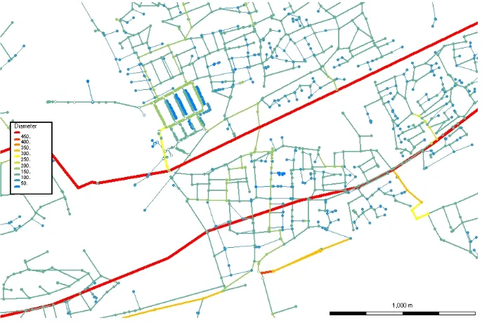
Figure 1. Part of a distribution network. The line colour and thickness represent the diameter of the pipes, the blue circles are demand nodes, open circles are nodes with zero demand. The thick yellow, orange and red lines are typically mains with a transport function (i.e. large diameters and very few demand nodes that are directly connected to it); the thin blue and green lines are mains with a distribution function (i.e. supply to customers).
network therefore, requires only a relatively simple hydraulic model (e.g. EPANET) which can be constructed from ba-sic pipe information (diameters, lengths and pipe material) and driven by strongly correlated demand profiles applied to nodes. The model is typically calibrated with pressure mea-surements (Kapelan, 2002).
Distribution mains have many demand nodes and instan-taneous demands among individual homes show little auto and cross correlation (Filion et al., 2006). A distribution net-work is usually designed for fire flow demands, that typically are much higher than domestic demand (Vreeburg, 2007). Therefore, under normal operating conditions, the maximum velocities in distribution mains can be very low (smaller than 0.01 m/s) and change rapidly. Flow directions may reverse and travel times may be as long as 100 h due to stagnation (Buchberger et al., 2003; Blokker et al., 2006). In the dis-tribution portion of the network, sediment does settle and re-suspend (Blokker et al., 2007; Vreeburg, 2007). This means a distribution mains model may need a rather complex struc-ture of demand allocation.
In modelling water quality in the DWDS the essential as-pects are transport, mixing, production and decay. Sedi-ment behaviour, and thus discolouration risk, in a DWDS is strongly related to hydraulics (Slaats et al., 2003; Vreeburg, 2007). The spread of dissolved contaminants through the DWDS is strongly related to the flows through the network (Grayman et al., 2006). The current water quality models are only validated for the transport network. Because consumers are located in the distribution part of the network, a water
quality model at that level is important. Because flows are more variable in the periphery of the DWDS, water quality models at this level may require a different approach than the current water quality models.
The key element to a water quality model for a DWDS is an accurate hydraulic model and therefore detailed knowl-edge of water demands is essential. This paper reviews the influence of (stochastic) demands on water quality models and the consequential constraints on demand modelling. Fol-lowing first, is a review of water quality modelling of dis-solved matter and its relation with demands. Next, water quality modelling of particulate matter and the relation with hydraulic conditions is described. Thirdly, the characteristics of demands in hydraulic network models and in network wa-ter quality models are discussed. Afwa-ter that, some demand models are considered.
2 Water quality modelling – dissolved matter
Water quality in a network model can be described with the Advection-Dispersion-Reaction (ADR) equation:
∂C ∂t +u
∂C ∂x =E
∂2C
∂x2 +f (C) (1)
where C is the cross-sectional average concentration (the wa-ter quality paramewa-ter, usually in mg/L), t is the time (s), u is the mean flow velocity (m/s), x is the direction of the flow, E represents the mixing (axial dispersion) coefficient in one-dimensional flow (m2/s) and f (C) is a reaction func-tion. The left-hand term of this equation depicts the advec-tion and mainly depends on bulk movement of the water. The first term on the right-hand side depicts the dispersion and the last term represents the reaction; both terms on the right-hand side of Eq. (1) depend on the type and nature of the considered substance. The reaction function can be very di-verse for different substances. In most instances, however, a simple first-order reaction is assumed, e.g. for chlorine de-cay, f (C)=−KC with K the reaction constant. The reaction function can include a production term.
The hydraulic network solver EPANET (Rossman, 2000) comes with a water quality module, as do many commer-cially available network analysis programs. The water qual-ity module enables the user to calculate travel times and to model the migration of a tracer (both conservative and non-conservative) through a network. It models advection and reaction with the pipe wall and the bulk of the water, but it does not take dispersion into account (i.e. neglects the first term of the right-hand side of the ADR equation). While EPANET can handle many different time scales (i.e. time in-tervals over which demands are time-averaged), a time scale of one hour is commonly used. The solver assumes that the network is well defined (known pipe diameter, pipe rough-ness and network layout), that demands are known, and that water quality reactions (under influence of residence times and interaction with the pipe wall) are known. Furthermore, EPANET assumes perfect mixing at junctions and steady-state hydraulic conditions during every computational inter-val. Hence, EPANET is not suitable for simulating transient flow in pipe networks. The accuracy of the calculated results depends on the validity of these assumptions.
To progress the water quality models, research is done on several of the assumptions in the models. In this review, the focus is on model deficiencies with respect to flows and ve-locities.
With respect to advection, Eq. (1) shows that time, and thus travel time, is an important factor as is the velocity of the water. A proper assumption of demands is a key factor in solving Eq. (1). Several authors (Pasha and Lansey, 2005; Filion et al., 2005; McKenna et al., 2005) have shown the im-portance of uncertainty in demands in water quality models. The needed detail in demand allocation is yet unknown.
Advection is also related to mixing. The conventional assumption of perfect mixing at junctions has been stud-ied with measurements and Computational Fluid
Dynam-ics modelling (Austin et al., 2008; Romero-Gomez et al., 2008a). The studies showed that at T-junctions, that are at least a few pipe diameters apart, perfect mixing can be as-sumed, while in cross junctions less than 10% mixing may occur. In fact, at cross junctions, the rate of mixture in the two outgoing arms depends on the Reynolds numbers (and thus the flow rates) in the two incoming arms.
When looking at smaller time steps a steady state as-sumption may not be valid. Karney et al. (2006) investi-gated the modelling of unsteadiness in flow conditions with several mathematical models such as extended period ap-proaches (like EPANET does), a rigid water column model that includes inertia effects, and a water hammer model that includes small compressibility effects. The time scale of boundary and flow adjustments relative to the water hammer time scale were found to be important for characterising the system response and judging the unsteadiness in a system. When for certain applications the required time step would be shorter than several minutes, the impact of taking inertia and compressibility into account should be studied further. The dispersion term in Eq. (1) is small in case of turbulent flow, but cannot be neglected in case of laminar flow. Gill and Sankarasubramanian (1970) derived an exact but cum-bersome expression showing that the instantaneous rate of dispersion in fully-developed steady laminar flow grows with time and asymptotically approaches the equilibrium disper-sion rate ETgiven by Taylor (1953),
ET =
d2u2
192D (2)
where D is the molecular diffusivity of a solute (m2/s) and d is the pipe diameter (m). Lee (2004) simplified the 1970 G&S result and provided a theoretical approximation for the time-averaged unsteady rate of dispersion, E(t), for a solute moving in steady laminar flow through a pipe,
E (t)=ET
"
1−1−exp [−16T (t)]
16T (t) #
(3) Here T (t)=4Dt/d2 is dimensionless Taylor time and t repre-sents the mean travel time through the pipe. When Taylor time is large, Eq. (3) reduces to Eq. (2). For nearly all net-works links, however, Taylor time is very small [e.g., T (t)< 0.01]. In this case, the expression in Eq. (3) can be further simplified,
E (t)≈ u
2t
6 = uL
6 (4)
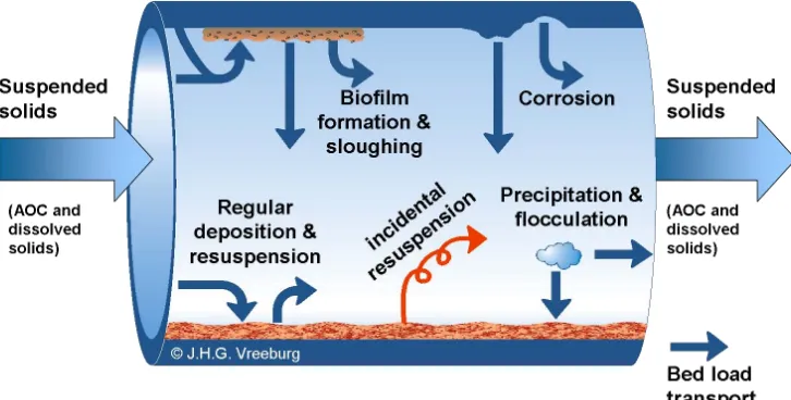
Figure 2.Processes related to particles in the distribution network.
time is T(t=15 000 s)=0.0027. For this condition, Eqs. (3) and (4) give similar results, namely, E(t)=0.1105 m2/s and 0.1117 m2/s, respectively. These estimates of the dispersion rate are eight orders of magnitude greater than the rate of molecular diffusivity. However, they are only two percent of the equilibrium value given by Taylor’s formula in Eq. (2), ET=5.26 m2/s. Owing to small molecular diffusivity and
rel-atively large pipe diameters, it is virtually impossible in real water distribution systems for the time-averaged rate of lami-nar dispersion to attain the equilibrium value given in Eq. (2). Recent preliminary experimental evidence indicates that Eqs. (3) and (4) tend to slightly over-estimate the actual time-averaged rate of dispersion observed in controlled laboratory runs (Romero-Gomez et al., 2008b). The reason(s) for this discrepancy are not clear and this is the subject of ongoing research investigations.
The influence of dispersion in water quality modelling was tested with (two-dimensional) ADR models (Tzatchkov et al., 2002; Li, 2006). Li (2006) showed that dispersion is important in laminar flows and thus especially in the parts of DWDS that have pipe diameters designed for fire flows but with small normal flows. Dispersion is not directly affected by flow pattern or time scale, although the tests of Romero-Gomez et al. (2008b) seem to suggest that the dispersion co-efficient is related to the Reynolds number. Flow pattern and time scale do, however, affect the probability of stagnation, laminar and turbulent flows, and thus indirectly do have an effect on dispersion.
Powell et al. (2004) have established that there is a need to further investigate the reaction parameters for chlorine decay, disinfectant by-products and bacterial regrowth. Where the reaction constant K involves a reaction with the pipe wall, the stagnation time is of importance. Flow velocities are impor-tant as they affect chlorine decay rates (Menaia et al., 2003).
3 Water quality modelling – particulate matter
For particulate matter the ADR model also applies; the re-action function for sediment includes a velocity term. In the gravitational settling model (Ryan et al., 2008) a parti-cles cloud is assumed, defined by a non-dimensional partiparti-cles cloud height s (proportional to the pipe diameter). When all particles are settled, s=0. When the flow velocity is larger than a certian threshold velocity (urs, the re-suspension
ve-locity) all particles are in suspesnion and s=1. When the flow velocity is smaller than a certian threshold velocity (ud,
the deposition velocity) particles settle with a downward ve-locity (us, the settling velocity) and 0<s<1:
s (t+ ∆t)=s (t)−us∆t
d , for u<ud (5)
In the particle wall deposition model (Ryan et al., 2008) the deposition of particles onto the pipe wall is caused by par-ticle/pipe surface attractive forces, e.g. Van der Waals force. The concentration of particles in suspension (C, in mg/L) can be described as follows:
∂C
∂t =−α(C−C∞) (6)
Hereαis a decay coefficient (s−1) and C∞is the final steady state concentration of particles (mg/L). C∞=βCw, with Cw
the mass of particles on the wall, per unit volume of water (mg/L) andβthe dimensionless wall mass coefficient.
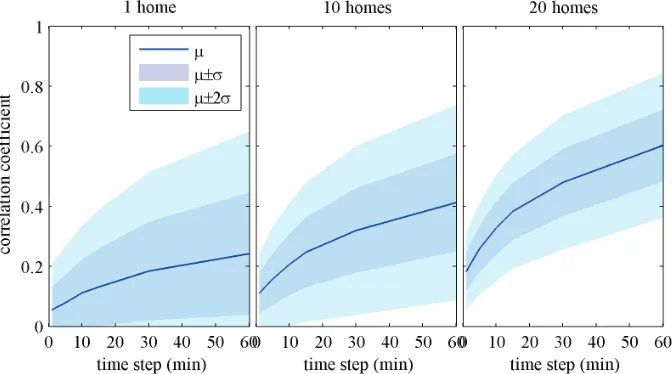
Figure 3.Mean (µ) and variation (σ) of cross correlation of measured patterns (Milford, OH) on different temporal scales and spatial scales; (a) 1 home, (b) 10 homes and (c) 20 homes.
third is to remove sediment by cleaning (flushing) the DWDS in a timely manner.
Although these three steps have proven to reduce the dis-colouration risk, the exact relation between the hydraulics and sediment behaviour (under what conditions does it settle and resuspend) is still unknown. More insight into the hy-draulic conditions can further support the second and third step.
Self-cleaning distribution networks (step 2) are effective because a regularly occurring threshold velocity prevents sediment from accumulating in the network. The threshold design velocity for self-cleaning DWDS is set to 0.4 m/s. Lab tests in the Netherlands (Slaats et al., 2003) have shown that sediment is partly resuspended at velocities of 0.1 to 0.15 m/s and fully resuspended at velocities of 0.15 to 0.25 m/s. In Australia, Grainger et al. (2003) have researched settle-ment and resuspension velocities. Settlement was found at 0.21 m/s (at which it could take several hours to a few days before all sediment was settled) and resuspension was found at 0.3 m/s. Field measurements in the Netherlands in 2006 have shown that the self-cleaning concept is feasible (Blokker et al., 2007; Vreeburg, 2007). The study suggests that the assumed design velocity of 0.4 m/s might be a con-servative value and a regular (i.e. a few times per week) oc-curring velocity of 0.2 m/s or less may be enough. The field measurements also showed that the current method to calcu-late the maximum flow (the so called q√n method; Vreeburg, 2007) overestimates the regular occurring flow, meaning that the regular flow for which the DWDS is designed (almost) never takes place. Since sediment behaviour is related to in-stantaneous (peak) flows, modelling of sediment in the net-work requires short time scales.
The self-cleaning design principles have mainly been ap-plied to the peripheral zones of the distribution system which
can be laid out as branched networks (sections of up to 250 residential connections). Even though the q√n method over-estimates the flows and the design velocity of 0.4 m/s might be a conservative value, the combination of these rules leads to self-cleaning networks (Blokker et al., 2007). In order to scale up the self-cleaning principles to the rest of the (looped) network it is important to look into a better estimate of the regular occurring maximum flows, because the q√n method cannot easily be applied in looped networks. Buchberger et al. (2008) have used the PRP model (Buchberger et al., 2003) to derive that the maximum flow equals “k1n+k2
√
n”, with n the number of homes and the constants k1and k2are related to the PRP parameters (see Sect. 5). Also, more research must be done on the relation between hydraulics and sedi-ment resuspension (i.e. establish the actual self-cleaning ve-locity).
To determine which part of the DWDS needs cleaning (step 3) several measurement techniques are available to de-termine where in the DWDS the discolouration risk is the highest (Vreeburg and Boxall, 2007); one example is the Re-suspension Potential Method (Vreeburg et al., 2004). Also, some models are being developed for this purpose. Boxall and Saul (2005) have developed a “predictor of discoloura-tion events in distribudiscoloura-tion systems” (PODDS). This model is based on the assumption that normal hydraulics forces (i.e. maximum daily shear stress) condition the sediment layer strength and hence control the discolouration potential (or discolouration risk).
4 Demands in hydraulic network models
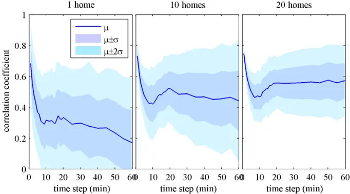
Figure 4.Mean (µ) and variation (σ) of lag-1 auto correlation coefficient of measured patterns (Milford, OH) on different temporal scales and spatial scales; (a) 1 home, (b) 10 homes and (c) 20 homes.
network modelling can be distinguished. The highest level is for planning the operation of the treatment plant, for which it is important to model the demand per day and for the to-tal supply area of a pumping station. The second level is modelling on transport level or to the level to which the as-sumption of cross correlation is still sufficient while for wa-ter quality modelling on a distribution level (the third level) a time scale on the order of minutes may be important (Li and Buchberger, 2004; Blokker et al., 2006).
Temporal and spatial aggregation of demands is related to cross and auto correlation of flows. A high cross correla-tion means that demand patterns at different nodes are similar (flows are proportional to each other). A high auto correla-tion is found when flow patterns change gradually. Cross and auto correlation thus are related to maximum flow rates and the stagnation time. This does not only influence water qual-ity; the amount of cross correlation is important with respect to the reliability of a DWDS (Filion et al., 2005) and thus the cost (Babayan et al., 2005); auto correlation is impor-tant with respect to the resilience of a DWDS, i.e. the time to restore service after a break (Filion et al., 2005). Sev-eral authors (Moughton et al., 2006; Filion et al., 2006; Li and Buchberger, 2007) have looked at the effect of temporal and spatial aggregation of demands on cross and auto corre-lation. They have shown that the longer the time scale and the higher the aggregation level, the higher the (cross) cor-relation. When looking at time scales of 1 h and demand nodes that represent 10 or more connections the assumption of cross correlation is valid. This means that strongly corre-lated demand patterns can be applied in the hydraulic model. Figures 3 and 4 show the mean and variance (µ±σ, repre-senting the 70% confidence interval andµ±2σ,the 95% con-fidence interval) of cross and lag-1 auto correlation coeffi
-cient for different time scales (1 to 60 min) and spatial scales (1, 10 and 20 homes per demand node) of 50 demand pat-terns as were measured in 1997 in 21 homes in Milford, Ohio (Buchberger et al., 2003). It shows that the cross correla-tion for demand patterns of individual homes or at short time steps are low (the lower bound of the 95% confidence inter-val is not above 0) and that only for 20 homes and 15 min, the lower bound of the 95% confidence interval of the cross correlation is above 20%. The lag-1 auto correlation coeffi -cient for short time steps can be high due to the high number of instances of zero flow. With increasing time step, the lag-1 auto correlation coefficient at first decreases with a decrease in zero flow instances and then increases with longer time steps, which is related to a more gradually changing pattern. For individual homes the lag-1 auto correlation coefficient is low (the lower bound of the 95% confidence interval is not above 0) due to the stochastic nature of the water use. For 10 homes or more, the average lag-1 auto correlation coefficient is stable at a time step of ca. 15 min or more, based on data from the Milford field study.
0 15 30 45 60 0
0.2 0.4 0.6 0.8 1
time step (min)
probability of stagnation
0 15 30 45 60 0
0.2 0.4 0.6 0.8 1
time step (min)
probability of laminar flow
0 15 30 45 60 0
0.2 0.4 0.6 0.8 1
time step (min)
probability of turbulent flow
1 5 10 20 50 100 150 200 # homes
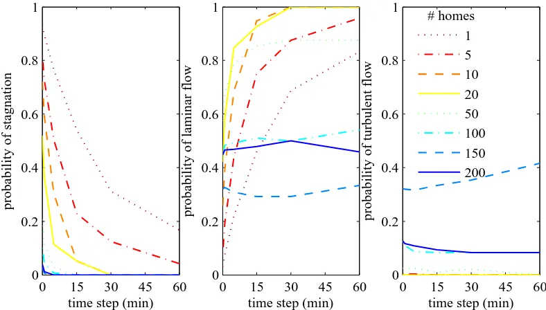
Figure 5.Probability of stagnation (Re=0), laminar flow (Re<2000) and turbulent flow (Re>4000) for different time steps and number of homes (1, 5 homes: Ø59 mm; 10 homes: Ø100 mm; 20, 50, 100, 150 homes: Ø150 mm; 200: Ø300 mm). The demand patterns that were used to construct these graphs were simulated with SIMDEUM (Blokker and Vreeburg, 2005; Blokker, 2005).
from several pressure events using different models of de-mand aggregation. The model results could be improved (compared to available field data) by artificially damping the residual pressure waves and by increasing instantaneous ori-fice demands. This means that in transient models insight into demands is very important. Skeletonisation also has an impact on hydraulic transient models (Jung et al., 2007), es-pecially in modelling the periphery of the distribution net-work (as opposed to the larger diameter pipes or transport network).
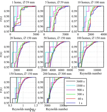
The flow variance and scale of fluctuation, the probability of stagnation and the flow regime (laminar or turbulent flow) are affected by the time scale that is used in a water qual-ity model (McKenna et al., 2003; Li, 2006). Figure 5 shows for some typical (Dutch) flow patterns at different temporal scales and spatial scales (i.e. different number of downstream homes with appropriate pipe diameter) what the probability of stagnation, probability of laminar flow (Re<2,000) and probability of turbulent flow (Re>4,000) are. Above ca. 50 homes the time step has little effect on the probability of stagnation, laminar and turbulent flow. A small time step (<1 min) is mainly of interest in the end of the pipe system. Figure 6 shows, for the same demand patterns, the 95 to 100 percentile of the Reynolds number for different spatial and temporal scales. It makes clear that for determining the max-imum flow a 1 min time scale is necessary when demands from less than 200 homes are considered; if more than 200 homes are involved a time scale of 5 min suffices.
0 5000 0.95
0.96 0.97 0.98 0.99
F(x)
1 home, ∅ 59 mm
0 5000 0.95
0.96 0.97 0.98 0.99
5 homes, ∅ 59 mm
0 2000 4000 0.95
0.96 0.97 0.98 0.99
10 homes, ∅ 100 mm
2000 4000 0.95
0.96 0.97 0.98 0.99
F(x)
20 homes, ∅ 150 mm
2000 4000 6000 8000 0.95
0.96 0.97 0.98 0.99
50 homes, ∅ 150 mm
5000 10000 0.95
0.96 0.97 0.98 0.99
Reynolds number 100 homes, ∅ 150 mm
0.5 1 1.5
x 104 0.95
0.96 0.97 0.98 0.99
Reynolds number
F(x)
150 homes, ∅ 150 mm
5000 10000 0.95
0.96 0.97 0.98 0.99
Reynolds number 200 homes, ∅ 300 mm
3600 s 1800 s 900 s 300 s 60 s 1 s
Figure 6.Maximum Reynolds number (95 to 100 percentile) for different time steps and number of homes (1, 5 homes: Ø59 mm; 10 homes: Ø100 mm; 20, 50, 100, 150 homes: Ø150 mm; 200: Ø300 mm). The demand patterns that were used to construct these graphs were simulated with SIMDEUM (Blokker and Vreeburg, 2005; Blokker, 2005).
5 Demand modelling
For a water quality network model a stochastic demand model per (household) connection on a per minute or finer basis is needed. Today, two types of demand models are available that fulfil this requirement: the Poisson Rectangular Pulse model and the end-use model SIMDEUM.
Buchberger and Wu (1995) have shown that residential water demand is built up of rectangular pulses with a certain intensity (flow) and duration arriving at different times on a day. The frequency of residential water use follows a Poisson arrival process with a time dependent rate parameter. When two pulses overlap in time, the result is the sum of the two pulses (Fig. 7). From extensive measurements it is possible to estimate the parameters to constitute a Poisson Rectangu-lar Pulse (PRP) model (Buchberger and Wells, 1996). Mea-surements were collected in the USA (Ohio; Buchberger et al., 2003), Italy (Guercio et al., 2001), Spain (Garc´ıa et al.,
2004) and Mexico (Alcocer-Yamanaka et al., 2006) and for each area the PRP parameters were determined. To estimate intensity and duration different probability distributions are applicable for different data sets, such as log-normal, expo-nential and Weibull distributions. Alvisi et al. (2003) use an analogous model based on a Neyman-Scott stochastic pro-cess (NSRP model) for which the parameters are also found from measurements. The PRP model is the basis for the de-mand generator PRPsym (Nilsson et al., 2005).
short pulses of 1 min or less, unless outdoor water use is also measured. This means that showering (ca. 10 to 15 min) is al-most never simulated as one continuous pulse. Another issue is that it is difficult to determine how well the simulation per-forms compared to the measurements, since the simulation parameters were derived from the same or similar measure-ments.
Another type of stochastic demand model is based on statistical information of end uses (Blokker and Vree-burg, 2005). The demand generator is called SIMDEUM (SIMulation of water Demand, an End Use Model). SIMDEUM simulates each end use as a rectangular pulse from probability distribution functions for the intensity, du-ration and frequency of use and a given probability of use over the day (related to presence at home and sleep-wake rhythm of residents, see Fig. 7). The probability distribution functions are derived from statistics of possession of water using appliance, their (water) use and population data (cen-sus data with respect to age and household size). The total simulated demand is the sum of all the end uses. SIMDEUM makes use of flow measurement data for validation only.
An end use model requires only a few demand measure-ments for validation. On the other hand, it requires statisti-cal data on water appliances and users, which are probably related to cultural differences and thus are nation specific. Because SIMDEUM is based on statistical information on in-home installation and residents, the influence of an aging population or replacement of old appliances with new ones can be determined easily and the model can easily be trans-ferred to other networks. SIMDEUM was applied and tested with good results in the Netherlands (Blokker and Vreeburg, 2005; Blokker et al., 2006).
SIMDEUM was also applied to Milford, Ohio, and com-pared to the extensive measurements that are available; also the PRP model and SIMDEUM were compared (Blokker et al., 2008). The basics for both models can be described by the following equations (Fig. 7):
Q=XB (I,D, τ) (7)
B(I,D, τ)= (
I τ <T < τ+D
0 elsewhere (8)
with D the pulse duration (in seconds), I the pulse intensity (flow in L/s) andτthe time at which the tap is opened. B(I, D,τ) is a block function, which equals I at timeτtoτ+D and 0 during the rest of the day. The summation is done for all pulses. The PRP model assumes a lognormal probability dis-tribution for the duration and intensity, with equal parameters for all pulses. The number of pulses follow a Poisson arrival process, and the average can vary per hour. SIMDEUM uses probability distributions of duration, intensity and number of pulses depending on the type of end-use, with parameters that may depend on the age of the resident or the number of residents per household. Blokker et al. (2008) showed that
the simulation results from both models fit the measured flow data very well. The PRP model uses flow measurements and accordingly represents the measured data well. The end-use model SIMDEUM uses sociologic data of the region under study; the required data for Milford could easily be collected, except for the specific time use data. With respect to the de-mand patterns of the single home SIMDEUM performs bet-ter than the PRP model on the aspects of maximum flow per second, the number of clock hours of water use and cross correlation. With respect to the demand patterns of the sum of 20 homes the PRP model works better than SIMDEUM on the aspect of fitting the diurnal pattern. The PRP model is a descriptive model, whereas SIMDEUM is more of a predic-tive model. Accordingly, the two models have different areas of application.
6 Discussion
Network water quality models on the distribution level may require fixture level or household level demands with no sig-nificant auto and cross correlation. This means that these models call for demand allocation via a bottom-up approach, i.e. allocating stochastic demand profiles with a small spatial aggregation level and appropriate short time scales.
There is currently no hydraulic network model that can properly work with instantaneous demands (i.e., on a per sec-ond basis) across an entire municipal network. Hence, even when nodal demands are known on a per second basis, they need to be integrated or averaged over a suitable time step before they can be used in a current network model. The best time step for hydraulic analysis will differ from the best time step for water quality analysis or human exposure analysis, and is related to the spatial aggregation level. When max-imum flows are of importance (e.g. in sediment behaviour modelling) a suitable time step is one minute when less than 200 homes are considered; for larger spatial aggregation lev-els five minutes would suffice, based on typical Dutch flow patterns. When the probability of stagnation is of importance (e.g. for modelling dissolved substances that are under the in-fluence of dispersion and interact with the pipe wall) a suit-able time step is one minute when less than 20 homes are considered; for more than 50 homes a one hour time step would suffice, based on data from the Milford field study. The question of the most suitable time step for network anal-ysis needs further investigation. Also, the influence of using instantaneous demands on transient effects, water compress-ibility, pipe expansion, inertia effects, etc. in network mod-els needs to be explored. Starting from very detailed network models with demands allocated per individual home and with time steps as short as one second, the effect of skeletonising and time averaging can be determined for different modelling purposes.
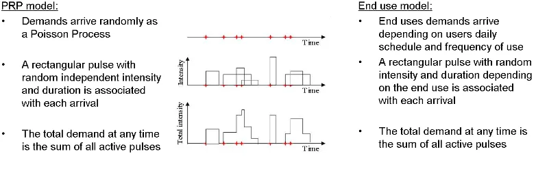
Figure 7.Schematic of the PRP and end use demand models. In the PRP model the Poisson arrival rate, intensity and duration are based on the measurements of pulses (similar to the lower diagram). In the end use model the arrival rate, intensity and duration are based on statistical information of end uses (toilet flushing, showering, washing clothes, doing the dishes, etc.)
(McKenna et al., 2005; Blokker et al., 2006). So far, little water quality measurements were done to validate the model results. Li (2006) has applied PRPSym in combination with EPANET and an ADR-model to compare the model to mea-surements of fluoride and chlorine concentrations in a net-work. The ADR-model with the stochastic demand patterns gave good results with the conservative fluoride and reason-able results with decaying chlorine. In particular, predicted concentrations in the peripheral zone of the network showed much better agreement with field measurements for the water quality model with dispersion (ADR) than for the water qual-ity model without dispersion (AR). Still, more network water quality models with stochastic demand should be tested with field data. This will reveal the shortcomings of the models and will indicate where improvement is to be gained. It will also provide more insight in the most suitable time step and spatial aggregation level for modelling.
Pressure measurements do not suffice for calibrating a network water quality model. Calibrating hydraulic mod-els on pressure measurements typically means adjusting pipe roughness. This only affects pressures and not flows. Adjust-ing flows from pressure measurements is too inaccurate. An accuracy of 0.5 m in two pressure measurements leads poten-tially to an uncertainty of 1 m in head loss. On a total head loss of only 5 m this is a 20% imprecision in pressure and thus a 10% imprecision in flow. Calibrating a network water quality model requires flow or water quality measurements, e.g. through tracer studies (Jonkergouw et al., 2008).
With the use of stochastic demands in a network model the question arises if a probabilistic approach on network modelling is required and how to interpret network simula-tions. Nilsson et al. (2005) demonstrated that Monte Carlo techniques are a useful tool for simulating the dynamic per-formance of a municipal drinking-water supply system, pro-vided that a calibrated model of realistic network operations is available. A probabilistic approach in modelling and in-terpreting results is a significant departure from prevailing
practice and it can be used to complement rather than replace current modelling techniques.
7 Summary and conclusions
Today, there is a growing interest in network water quality modelling. The water quality issues of interest relate to both particulate and dissolved substances, with the main interest in sediment leading to discolouration, respectively in residual chlorine and contaminant propagation. There is a strong in-fluence of flows and velocities on transport, mixing, produc-tion and decay of these substances in the network which im-poses a different approach to demand modelling. For trans-port systems the current hydraulic (AR) models suffice; for the more detailed distribution system a network water qual-ity model is needed that is based on short time scale demands that considers the effect of dispersion (ADR) and transients. Demand models that provide trustworthy stochastic residen-tial demands per individual home and on a one-second time scale are available.
The contribution of dispersion in network water quality modelling is significant. The contribution of transients in network water quality modelling still needs to be established. A hydraulics based, or rather a stochastic demands based, network water quality model needs to be developed and validated with field measurements. Such a model will be probabilistic in nature and will lead to a whole new way of assessing water quality in the DWDS.
References
Alcocer-Yamanaka, V. H., Tzatchkov, V. G., and Buchberger, S. G.: Instantaneous water demand parameter estimation from coarse meter readings, Water Distribution System Analysis #8., Cincin-nati, Ohio, USA, 2006, 2006.
Alvisi, S., Franchini, M., and Marinelli, A.: A Stochastic Model for Representing Drinking Water Demand at Residential Level, Water Resour. Manag., 17, 197–222, 2003.
Austin, R. G., Waanders, B. v. B., McKenna, S., and Choi, C. Y.: Mixing at cross junctions in water distribution systems. II: exper-imental study, J. Water Res. Pl.-Asce, 134, 295–302, 2008. Babayan, A. V., Savic, D. A., and Walters, G. A.: Multiobjective
optimization for the least-cost design of water distribution sys-tem under correlated uncertain parameters, Impacts of Global Climate Change; 2005 World water and environmental resources congress, Anchorage, Alaska, 2005.
Blokker, E. J. M.: Determining the capacity of drinking water dis-tribution systems at street level, Kiwa N. V., Nieuwegein, 2005 (in Dutch).
Blokker, E. J. M. and Vreeburg, J. H. G.: Monte Carlo Simula-tion of Residential Water Demand: A Stochastic End-Use Model, Impacts of Global Climate Change; 2005 World water and envi-ronmental resources congress, Anchorage, Alaska, 15–19 May 2005.
Blokker, E. J. M., Vreeburg, J. H. G., and Vogelaar, A. J.: Combin-ing the probabilistic demand model SIMDEUM with a network model, Water Distribution System Analysis #8, Cincinnati, Ohio, USA, 27–30 August 2006.
Blokker, E. J. M., Vreeburg, J. H. G., Schaap, P. G., and Horst, P.: Self-cleaning networks put to the test, World environmental and water resources congress 2007 - Restoring our natural habitat, Tampa, Fl, USA, 15–18 May 2007.
Blokker, E. J. M., Buchberger, S. G., Vreeburg, J. H. G., and van Dijk, J. C.: Comparison of water demand models: PRP and SIMDEUM applied to Milford, Ohio, data., WDSA 2008, Kruger Park, South Africa, August 2008.
Bowden, G. J., Nixon, J. B., Dandy, G. C., Maier, H. R., and Holmes, M.: Forecasting chlorine residuals in a water distri-bution system using a general regression neural network, Math. Comput. Model., 44, 469–484, 2006.
Boxall, J. B. and Saul, A. J.: Modeling Discoloration in Potable Water Distribution Systems, J. Environ. Eng. ASCE, 131, 716– 725, 2005.
Buchberger, S. G. and Wu, L.: Model for Instantaneous Residential Water Demands, J. Hydraul. Eng.-ASCE, 121, 232–246, 1995. Buchberger, S. G. and Wells, G. J.: Intensity, duration and
fre-quency of residential water demands, J. Water Res. Pl-ASCE, 122, 11–19, 1996.
Buchberger, S. G., Carter, J. T., Lee, Y. H., and Schade, T. G.: Random demands, travel times, and water quality in dead ends, American Water Works Association Research Foundation, Den-ver, Colorado, USA, 2003.
Buchberger, S. G., Blokker, E. J. M., and Vreeburg, J. H. G.: Sizes for Self-Cleaning Pipes in Municipal Water Supply Systems, WDSA 2008, Kruger Park, South Africa, August 2008. Filion, Y. R., Karney, B. W., and Adams, B. J.: Stochasticity of
de-mand and probabilistic performance of water networks, Impacts of Global Climate Change; 2005 World water and environmental
resources congress, Anchorage, Alaska, 2005, 49, 2005. Filion, Y. R., Karney, B. W., Moughton, L. J., Buchberger, S. G.,
and Adams, B. J.: Cross correlation analysis of residential de-mand in the city of Milford, Ohio, Water Distribution System Analysis #8, Cincinnati, Ohio, USA, 2006.
Garc´ıa, V., Bartual, R., Cabrera, E., Arregui, F., and Garc´ıa-Serra, J.: Stochastic model to evaluate residential water demands, J. Water Res. Pl.-ASCE, 130, 386–394, 2004.
Gill, W. N. and Sankarasubramanian, R.: Exact analysis of unsteady convective diffusion, P. Roy. Soc. Lond. A. Mat., 316, 341–350, 1970.
Grainger, C., Wu, J., Nguyen, B. V., Ryan, G., Jayaratne, A., and Mathes, P.: Particles in water distribution systems – 5th progress report; part I: settling, re-suspension and transport, CSIRO-BCE, Australia, 71 p., 2003.
Grayman, W. M., Speight, V. L., and Uber, J. G.: Using Monte-Carlo simulation to evaluate alternative water quality sampling plans, Water Distribution System Analysis #8, Cincinnati, Ohio, USA, 2006.
Guercio, R., Magini, R., and Pallavicini, I.: Instantaneous resi-dential water demand as stochastic point process, in: Water re-sources management, Progress in water rere-sources, 4, WIT Press, Southampton, UK, 129–138, 2001.
Jonkergouw, P. M. R., Khu, S.-T., Kapelan, Z. S., and Savic, D. A.: Water quality model calibration under unknown demands, J. Water Res. Pl-ASCE, 134, 326–336, 2008.
Jung, B., Boulos, P. F., and Wood, D. J.: Impacts of skeletonization on distribution system hydraulic transient models, World envi-ronmental and water resources congress 2007 – Restoring our natural habitat, Tampa, Fl, USA, 2007.
Kapelan, Z.: Calibration of water distribution system hydraulic models, University of Exeter, PhD thesis, 334 p., 2002. Karney, B. W., Jung, B., and Alkozai, A.: Assessing the degree of
unsteadiness in flow modeling; from physics to numerical solu-tion, Water Distribution System Analysis #8, Cincinnati, Ohio, USA, 2006.
Lee, Y.: Mass dispersion in intermittent laminar flow, University of Cincinnati, Cincinnati, Ohio, 167 pp., 2004.
Li, Z. and Buchberger, S. G.: Effect of time scale on PRP random flows in pipe network, Critical Transitions In Water And Envi-ronmental Resources Management, Salt Lake City, Utah, 2004, conference paper available on CD, doi:10.1061/40737(2004)461, 2004.
Li, Z.: Network Water Quality Modeling with Stochastic Water De-mands and Mass Dispersion, University of Cincinnati, PhD the-sis, 166 p., 2006.
McInnis, D. and Karney, B. W.: Transients in distribution networks: Field tests and demand models, J. Hydraul. Eng., 121, 218–231, 1995.
McKenna, S. A., Buchberger, S. G., and Tidwell, V. C.: Examining the effect of variability in short time scale demands on solute transport, World Water and Environmental Resources Congress and Related Symposia, Philadelphia, Pennsylvania, USA, 2003. McKenna, S. A., van Bloemen Waanders, B., Laird, C. D.,
Buch-berger, S. G., Li, Z., and Janke, R.: Source location inversion and the effect of stochastically varying demand, Impacts of Global Climate Change; 2005 World water and environmental resources congress, Anchorage, Alaska, 2005, 47, 2005.
De-pendency of bulk chlorine decay rates on flow velocity in wa-ter distribution networks, Wawa-ter Science and Technology: Wawa-ter Supply, 3, 209–214, 2003.
Nilsson, K. A., Buchberger, S. G., and Clark, R. M.: Simulating exposures to deliberate intrusions into water distribution systems, J. Water Res. Pl.-ASCE, 131, 228–236, 2005.
Pasha, M. F. K. and Lansey, K.: Analysis of uncertainty on wa-ter distribution hydraulics and wawa-ter quality, Impacts of Global Climate Change; 2005 World water and environmental resources congress, Anchorage, Alaska, 2005.
Powell, J., Clement, J., Brandt, M., R, C., Holt, D., Grayman, W., and LeChevallier, M.: Predictive Models for Water Quality in Distribution Systems, AwwaRF, Denver, Colorado, USA, 132 p., 2004.
Propato, M. and Uber, J.: Vulnerability of Water Distribution Sys-tems to Pathogen Intrusion: How Effective Is a Disinfectant Residual?, Environ. Sci. Technol., 38, 3713–3722, 2004. Romero-Gomez, P., Ho, C. K., and Choi, C. Y.: Mixing at cross
junctions in water distribution systems. I: numerical study, J. Wa-ter Res. Pl.-ASCE, 134, 285–294, 2008a.
Romero-Gomez, P., Li, Z., Choi, C. Y., Buchberger, S. G., Lansey, K. E., and Tzatchkov, V. T.: Axual dispersion in a pressurized pipe under various flow conditions, WDSA 2008, Kruger Park, South Africa, August 2008b.
Rossman, L. A., Clark, R. M., and Grayman, W. M.: Modeling chlorine residuals in drinking-water distribution systems, J. Env-iron. Eng., 120, 803–820, 1994.
Rossman, L. A.: EPANET 2 user manual, United States Environ-mental Protection Agency, Cincinnati, 200 p., 2000.
Ryan, G., Mathes, P., Haylock, G., Jayaratne, A., Wu, J., Noui-Mehidi, N., Grainger, C., and Nguyen, B. V.: Particles in wa-ter distribution systems, Cooperative Research Centre for Wawa-ter Quality and Treatment, Salisbury, Australia, 106 pp., 2008. Slaats, P. G. G., Rosenthal, L. P. M., Siegers, W. G., van den
Boomen, M., Beuken, R. H. S., and Vreeburg, J. H. G.: Processes involved in the generation of discolored water, Awwa Research Foundation, Denver, Co, USA, 2003.
Taylor, G.: Dispersion of Soluble Matter in Solvent Flowing Slowly through a Tube, P. Roy. Soc. Lond. A Mat., 219, 186–203, 1953. Tzatchkov, V. G., Aldama, A. A., and Arreguin, F. I.: Advection-dispersion-reaction modeling in water distribution networks, J. Water Res. Pl.-ASCE, 131, 334–342, 2002.
Tzatchkov, V. G., and Buchberger, S. G.: Stochastic demand gener-ated unsready flow in water distribution networks, Water Distri-bution System Analysis #8, Cincinnati, Ohio, USA, 2006. USEPA: Initial Distribution System Evaluation Guidance Manual
for Final Stage 2 Disinfection Byproducts, Office of Water, 2006. Vreeburg, J. H. G., Schaap, P. G., and van Dijk, J. C.: Measuring discoloration risk: resuspention potential method, Leading edge Technology conference, Prague, 1–3 June 2004.
Vreeburg, J. H. G.: Discolouration in drinking water systems: a particular approach, PhD thesis, 183 p., 2007.