www.solid-earth.net/6/701/2015/ doi:10.5194/se-6-701-2015
© Author(s) 2015. CC Attribution 3.0 License.
Instaseis: instant global seismograms based on a broadband
waveform database
M. van Driel1, L. Krischer2, S. C. Stähler2,3, K. Hosseini2, and T. Nissen-Meyer4 1Dept. of Earth Sciences, ETH Zürich, Sonneggstrasse 5, 8092 Zurich, Switzerland
2Dept. of Earth Sciences, Ludwig-Maximilians-Universität München, Theresienstraße 41, 80333 Munich, Germany 3Leibniz-Institute for Baltic Sea Research, Warnemünde, Seestraße 15, 18119 Rostock, Germany
4Dept. of Earth Sciences, University of Oxford, South Parks Road, Oxford OX1 3AN, UK Correspondence to: M. van Driel ([email protected])
Received: 16 January 2015 – Published in Solid Earth Discuss.: 6 March 2015 Revised: 4 May 2015 – Accepted: 8 May 2015 – Published: 16 June 2015
Abstract. We present a new method and implementation (In-staseis) to store global Green’s functions in a database which allows for near-instantaneous (on the order of milliseconds) extraction of arbitrary seismograms. Using the axisymmetric spectral element method (AxiSEM), the generation of these databases, based on reciprocity of the Green’s functions, is very efficient and is approximately half as expensive as a single AxiSEM forward run. Thus, this enables the compu-tation of full databases at half the cost of the compucompu-tation of seismograms for a single source in the previous scheme and allows to compute databases at the highest frequencies glob-ally observed. By storing the basis coefficients of the numer-ical scheme (Lagrange polynomials), the Green’s functions are 4th order accurate in space and the spatial discretization respects discontinuities in the velocity model exactly. High-order temporal interpolation using Lanczos resampling al-lows to retrieve seismograms at any sampling rate. AxiSEM is easily adaptable to arbitrary spherically symmetric models of Earth as well as other planets. In this paper, we present the basic rationale and details of the method as well as bench-marks and illustrate a variety of applications. The code is open source and available with extensive documentation at www.instaseis.net.
1 Introduction
Despite the exponential growth of computational power and substantial progress of 3-D numerical methods for seis-mic wave propagation in the last 15 years (Igel et al.,
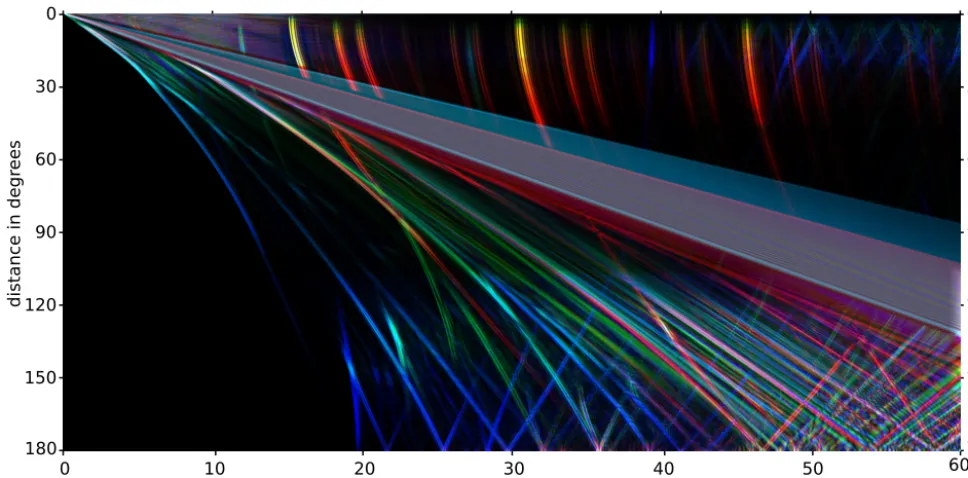
2000; Komatitsch and Tromp, 2002a; Tromp, 2007; Tromp et al., 2010), the simulation of the highest frequencies ob-served in seismic waves on the global scale remains a high-performance computing challenge and is not yet done rou-tinely. This is why many seismologists still rely on approxi-mate methods to compute and analyze high-frequency body waves such as ray-theoretical travel times (e.g. the TauP-toolkit described in Crotwell et al., 1999), WKBJ synthet-ics (Chapman, 1978), the reflectivity method (Fuchs and Müller, 1971) or the frequency–wave number integration method (Kikuchi and Kanamori, 1982). More recently, sev-eral methods that include the full physics in solving the seis-mic wave equation while reaching the highest observable fre-quencies by assuming spherically symmetric models have become available, see Fig. 1 for an example. These methods include the direct solution method (DSM, Geller and Ohmi-nato, 1994; Kawai et al., 2006), the frequency domain inte-gration method (GEMINI, Friederich and Dalkolmo, 1995) and a generalization of it including self gravitation (Yspec, Al-Attar and Woodhouse, 2008).
at-0
30
60
90
120
150
180
0 10 20 30 40 50 60
time in minutes
distanc
e in degr
ees
0
30
60
90
120
150
180
Figure 1. Global stack of 1 h of seismograms accurate to a shortest period of 2 s for an earthquake in 27 km depth computed with Instaseis.
The displacement is color-coded analogous to the IRIS global stack (Astiz et al., 1996), i.e. red: transversal component, green: radial compo-nent, blue: vertical component. An automatic gain control (AGC) with a window of 100 s length is used to balance large amplitude variations between the various phases. Note that creating this plot does not require to define the source depth at the time of database calculation. A high-resolution version of this plot and one for 5 h long seismograms is added as an electronic supplement.
tenuation (van Driel and Nissen-Meyer, 2014a, b), published under public license (Nissen-Meyer et al., 2014) and is avail-able at www.axisem.info.
As computing full global waveforms especially at higher frequencies requires substantial computational resources, several initiatives serve to deliver waveforms by means of databases without having to run a full numerical solver. The ShakeMovie project (http://global.shakemovie. princeton.edu) provides synthetics for earthquakes from the CMT (Global Centroid-Moment-Tensor) catalogue (www. globalcmt.org) recorded at permanent Global Seismic Net-work (GSN) and International Federation of Digital Seis-mograph Networks (FDSN) stations in 1-D and 3-D veloc-ity models (Tromp et al., 2010). The Pyrocko toolbox (http: //emolch.github.io/pyrocko) provides a Python interface to generate and access Green’s function databases, which for the global case are based on GEMINI, several databases are offered for download.
In this paper we present a method that uses AxiSEM to generate global Green’s function databases and provides a Python interface for convenient extraction of seismograms. The advantage over ShakeMovie synthetics are the pos-sible higher frequencies and arbitrary source and receiver combinations independent of catalogues and real stations. Compared to Pyrocko with GEMINI synthetics, AxiSEM is more efficient in generating the databases, allowing to routinely compute them for a large number of different
background models or specialized applications (e.g. limited depth/distance ranges). Also, by using the Lagrangian poly-nomials in the SEM (spectral element method) mesh as basis functions, it achieves higher spatial accuracy.
This paper is structured as follows. In Sect. 2 we present the technical aspects and argue for the choices made in the spatial and temporal discretization. Section 3 gives a short overview of the Python interface. In Sect. 4 we show the per-formance with respect to accuracy, speed and disk space re-quirements for the databases. Finally, we depict a variety of applications in Sect. 5.
2 Methods
Figure 2. The 3-D wave field is decomposed analytically into
monopole, dipole and quadrupole radiation patterns (left) and the remaining 2-D problem is solved on a D-shaped domain (right) us-ing the spectral element method. While the forward databases re-quire a total of four 2-D computations, it is only two for the back-ward databases using reciprocity of the Green’s function: one for the vertical and one for the horizontal components (modified from Nissen-Meyer et al., 2014).
when larger regions of Earth are included in the database. AxiSEM uses a spectral element scheme for spatial dis-cretization which lends itself well to parallelization on High Performance Computing (HPC) systems. As it is based on the weak formulation of the wave equation, it naturally includes the free surface boundary condition and allows for highly ac-curate modeling of surface waves.
Nissen-Meyer et al. (2014) argued against using collec-tive parallel I/O since the availability of the NetCDF li-braries (Rew and Davis, 1990) was not granted on all su-percomputers. For that reason, we implemented a round robin I/O scheme, which remains advantageous when run-ning AxiSEM on less than about 100 cores in parallel and to avoid installation problems on systems where NetCDF is not available as a pre-compiled package. On supercomputers however, the situation has since improved and NetCDF com-piled with parallel support seems now to be widespread. For this reason, we implemented a collective parallel I/O scheme that performs well, even when running on more than 1000 cores, see Table 1. In this scheme, all processes that have to write data to disk communicate via the message passing in-terface (MPI) and then write collectively at the same time to the parallel file system. This way we achieved throughputs of up to 4 GB s−1on SuperMUC.
1.0 0.5 0.0 0.5 1.0
or 0.2
0.0 0.2 0.4 0.6 0.8
1.0
n = 0
n = 1
n = 2
n = 3
n = 4
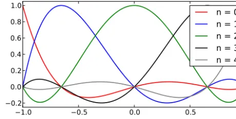
Figure 3. Lagrangian basis polynomialsln(ξ )of fourth order in one dimension. At the collocation points, all but one are zero, such that the value of the interpolated function at this point coincides with the coefficient in this basis expansion.
2.2 Forward and backward databases
Instaseis has the capability of dealing with forward wave fields, i.e. the waves are propagated from a moment-tensor point source at fixed depth (i.e. receivers exist throughout the medium), as well as backward or reciprocal wave fields, where the wave fields are propagated from a single-force point source at fixed depth and recorded throughout the medium (i.e. sources exist throughout the medium).
Potential applications of forward databases are the gen-eration of 3-D wave-propagation movies (Holtzman et al., 2013), the computation of incoming teleseismic waves in 1-D/3-D hybrid methods (e.g. Monteiller et al., 2012; Masson et al., 2013) or the forward field in the computation of sen-sitivity kernels (Nissen-Meyer et al., 2007a) for seismic to-mography. To generate a forward database, a total of four runs with AxiSEM are needed (Nissen-Meyer et al., 2007b). In contrast, reciprocal databases utilize the reciprocity of the Green’s functions, and are useful in all cases where the receivers are at fixed depth, thus for instance mimicking earthquake catalogues recorded at stations along the surface. The source can be located anywhere in the region where the Green’s functions are recorded in the simulation, thus allow-ing for unlimited choices in the source–receiver geometry. To generate a reciprocal database, a total of two runs with AxiSEM are needed, one for the vertical component and one for both horizontal components of the seismogram (Nissen-Meyer et al., 2007b). It is also possible to compute a database for the vertical component seismograms only, which is then a factor of 3 faster and uses only about 40 % of the disk space. 2.3 The spatial scheme
2 1 0 1 2 1.5
1.0 0.5 0.0 0.5 1.0 1.5
Figure 4. Lagrange interpolation points inside an element (gray)
and its neighbors. Coordinatesξandηare the reference coordinates of the gray element. Points on the edges (black squares) are shared between neighbors and function values at these points need to be stored only once if the function is continuous (e.g. displacement). The number of global degrees of freedom per element of such func-tions is thus approximately 16 compared to 25 for discontinuous functions (e.g. strain).
spectral element scheme (see Fig. 4):
u(ξ, η, t )=
N X
ij=0
uij(t )li(ξ )lj(η); (1)
ξ andηare the reference coordinates of the element andN
typically has a value of 4. This approach has several advan-tages.
– The wave field is represented by polynomials, typically of degree 4; interpolation is hence of 4th order accuracy. – The basis is local and only few coefficients are needed to represent the wave field inside an element (typically 25), in contrast to e.g. global basis functions such as spherical harmonics.
– Discontinuities in the model that cause discontinuities in the strain Green’s functions are respected by the mesh.
– The strain tensor (representing the moment tensor in the reciprocal case) can be computed on the fly from the stored displacements at high accuracy. This reduces the storage by a factor of 2 as the displacement has 3 de-grees of freedom, compared to 6 for the strain.
– Since the displacement is continuous also at model discontinuities and element boundaries, it needs to be stored only once at all Gauss–Lobatto–Legendre (GLL) points that belong to multiple elements, reducing the storage by another factor of 16/25=0.64 (see Fig. 4).
Green's function Grr,r / N
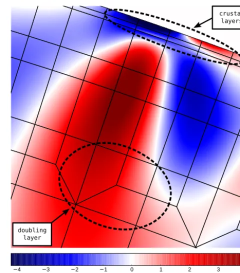
Figure 5. Snapshot of one component of the Green’s tensor (Grr,r) as represented in the SEM basis for a shortest period of 50s. Discon-tinuities such as caused by the crustal layers are exactly represented and the wave field is smooth across doubling layers of the mesh.
– Storing the displacement allows to use force sources as well without any extra computation or storage require-ments.
Figure 5 visualizes the spatial representation for a long pe-riod mesh (50 s) for the Rayleigh wave train and theGrr,r component of the strain Green’s tensor: the strain is smooth also across the doubling layer of the mesh where the back-ground model (ak135f, Montagner and Kennett, 1996) is smooth as well. Still, the discontinuities of the model and hence the strain are explicitly represented by this discretiza-tion and the resoludiscretiza-tion of the mesh is adapted to the local wavelength, as for instance in the crust. Figure 6 shows an example for 2 s shortest period and compares the SEM dis-cretization to regular depth sampling. In the regular sampling case with nearest neighbor interpolation, the phase and enve-lope errors can be quite large, especially close to the model discontinuities (up to 80 % envelope misfit and 4 % phase misfit as defined by Kristekova et al., 2009) and for very shallow sources (up to 40 % envelope misfit and 14 % phase misfit).
2.3.1 Finite element mapping
370 380 390 time / s 0
5
10
15
20
25
source depth / km
370 380 390 time / s
2 1 0 1 2
1e 24
1% 10% 100% EM PM Green's function Grr,r / N
a) b) c)
Figure 6. One component of the strain Green’s tensor (Grr,r) for a distance of 30◦as a function of time and depth with a shortest period of 2 s. (a) SEM basis vs. (b) regular sampling with 1 km distance and (c) phase and envelope misfits (EM and PM in the legend, see Kristekova et al., 2009) caused by the regular sampling computed in the period range 1–20 s. Dashed lines in the left panel sketch the spectral elements. The crustal discontinuities of ak135f (Montagner and Kennett, 1996) are indicated by solid lines and lead to disconti-nuities inGrr,r, which are exactly represented in the SEM basis.
the opposite mapping is trivial because this is how the ele-ments of the SEM are defined (Nissen-Meyer et al., 2007a, Appendix A1), it cannot be generally inverted easily. Hua (1990) presents an analytical inverse solution for quadrilat-eral elements, which is quite involved and not easy to gener-alize for the semicircular elements used in AxiSEM.
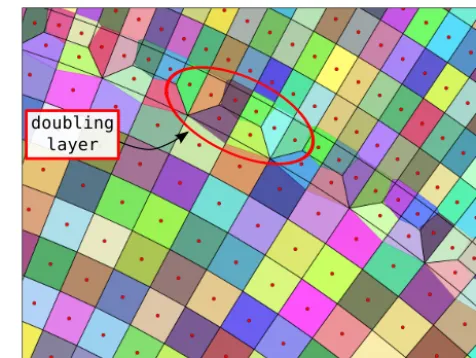
We follow a two-step approach to finding the reference coordinates. First, we find the six closest element midpoints to limit the search to a small number of candidate elements in which the point could be. The number six is specific to the AxiSEM mesh, where each corner point can belong to a maximum of six elements in the doubling layers, see Fig. 7. This step can be seen as approximating the AxiSEM mesh with Voronoi cells. For most points, the closest midpoint will already indicate the correct element, in the worst case the second step has to be performed for all six candidates.
Figure 7. Voronoi approximation (colored) of the AxiSEM mesh
(black lines) using the midpoints of the elements (red circles) only, zoomed onto a doubling layer for a 50 s mesh. For most elements, the Voronoi cell coincides almost exactly with the AxiSEM element, note that most of the AxiSEM elements have edges of concentric circles while the edges of the Voronoi cells are all straight lines. In the worst case, six AxiSEM elements have to be tested whether a point is inside or not.
In a second step, the reference coordinates (ξ, η) of the given point(sp, zp)are computed for the six candidate el-ements sorted by the distance of the midpoints. If both ξ
and η are in the interval [−1, 1], the element is found. The coordinates(ξ, η)are computed using an iterative gra-dient scheme adopted from SPECFEM3D (Komatitsch and Tromp, 2002b). Starting from the midpoint of the candidate element, updated values are found by linear approximation of the inverse mapping:
ξn+1
ηn+1
=
ξn
ηn
+J−1(ξ n, ηn)·
sp−s(ξn, ηn)
zp−z(ξn, ηn)
, (2)
with the Jacobian matrix defined as
J(ξ, η)=
∂ξs ∂ηs
∂ξz ∂ηz
, (3)
and the mappings(ξ, η) andz(ξ, η) depending on the ele-ment type as defined in Nissen-Meyer et al. (2007b). In the AxiSEM mesh, this iteration converges to numerical accu-racy within less than 10 iterations and is not performance critical for Instaseis as it is only used on the few candidate elements. Also, this two-step approach requires only the mid-points of all elements in the mesh to be read from file on ini-tialization and can be implemented efficiently using the kd-tree provided by the SciPy package (http://www.scipy.org/). 2.4 The temporal scheme
4 2 0 2 4 0.0
0.5 1.0
sinc a = 2
4 2 0 2 4
sinc a = 5
4 2 0 2 4
sinc a = 20
Figure 8. Lanczos kernels used for resampling. For large values of the parametera, it converges towards the sinc function, which is the kernel that allows exact reconstruction for bandlimited signals as stated in the Nyquist sampling theorem (Nyquist, 1928).
466 468 470 472 474
time / s 1.5
1.0 0.5 0.0 0.5 1.0
velocity / (m/s)
1e 7
original
downsampled
resampled
diff x 100
Figure 9. Resampling using a Lanczos kernel witha=12 of a P ar-rival velocity seismogram convolved with the source time function from Fig. 11 recorded at 40◦distance, and the resampling error mul-tiplied by a factor of 100. The relative error is on the order of 0.05 % of RMS, see Fig. 10.
0 5 10 15 20 25 30 35 40 a
10-4 10-3 10-2 10-1 100
RMS error
Figure 10. RMS error of the resampling using the first 1800 s of the
seismogram from Fig. 9. Convergence is reached arounda=20. It does not converge to zero because some high-frequency energy was neglected in the downsampling, see Fig. 11.
spectrum should decay steep enough above the highest fre-quency resolved by the mesh, such that the least number of samples according to the Nyquist criterion can be used with-out introducing aliasing. On the other hand, it should not de-cay too steeply, such that it is still possible to deconvolve and convolve with another source time function. Additionally, the spectrum should be as flat as possible within the usable fre-quency range as well as “earthquake-like” without the
ne-10-1 100
frequency / Hz 10-4
10-3 10-2 10-1 100
normalized amplitude spectrum mesh period
downsampling Nyquist
sliprate
seismogram
smoothed sg
Figure 11. Normalized amplitude spectra of the Gaussian source
time function (slip rate) used at 2 s mesh period and a vertical com-ponent synthetic seismogram recorded at 40◦ epicentral distance. The vertical lines denote the resolution of the mesh and the Nyquist frequency of the downsampling using four samples per mesh pe-riod.
cessity of deconvolution when extracting a seismogram from the database. An actual delta function as would be required for true Green’s functions cannot be represented in a discrete approximation as it is not bandlimited.
We found a Gaussian source time function withσ=τ/3.5 to fulfill these requirements, whereτ is the shortest period re-solved by the mesh. Figure 11 shows the amplitude spectra of this source time function as well as a corresponding velocity seismogram at a distance of 40◦. The two spectra have a very similar general shape and decay to 10−3of the maximum at half the shortest period. This motivates that sampling with four samples per period will not introduce aliasing artifacts.
>>> import instaseis
>>> db = instaseis.open_db("./AK135")
>>> receiver = instaseis.Receiver(network="BW", station="ZUGS", latitude=47.416, longitude=10.979) >>> source = instaseis.Source(
latitude=89.91, longitude=0.0, depth_in_m=12000, m_rr = 4.71e+17, m_tt = 3.81e+15, m_pp =-4.74e+17, m_rt = 3.99e+16, m_rp =-8.05e+16, m_tp =-1.23e+17) >>> st = db.get_seismograms(source=source, receiver=receiver) >>> print(st)
3 Trace(s) in Stream:
BW.ZUGS..LXZ | 1970-01-01T00:00:00.00Z - ... | 2.1 Hz, 7746 samples BW.ZUGS..LXN | 1970-01-01T00:00:00.00Z - ... | 2.1 Hz, 7746 samples BW.ZUGS..LXE | 1970-01-01T00:00:00.00Z - ... | 2.1 Hz, 7746 samples
Figure 12. The Instaseis Python API demonstrated in a short
in-teractive Python session. ASourceand aReceiverobject are created and then passed to theget_seismograms()method of anInstaseisDBobject. This will extract the Green’s functions from the databases and perform all necessary subsequent steps re-sulting in directly usable three-component seismograms in form of an ObsPyStreamobject. Please refer to the Instaseis documenta-tion for details.
Burger and Burge, 2009, Sect. 10.3 for an extended introduc-tion to interpolaintroduc-tion).
Therefore, we adopt the Lanczos resampling scheme, which is popular in image processing, and an approximation to the sinc-resampling with finite support. The Lanczos ker-nel is defined as the sinc function multiplied by the Lanczos window function (Burger and Burge, 2009):
L(t )=
(
sinc(t )sinc(t /a) ift∈ [−a, a]
0 else,, (4)
whereais a parameter to control the number of samples to be used in the interpolation and the sinc function is defined as
sinc(t )=sin(π t )
π t . (5)
Interpolation is then performed by convolving the discrete signalsi with this kernel and evaluating it at the new time samplestj(Burger and Burge, 2009):
S(tj)=
btj/1tc+a
X
i=btj/1tc−a+1
siL tj/1t−i
, (6)
whereb·cdenotes the floor function and1tthe sampling in-terval of the original signal. Figure 8 shows the Lanczos ker-nel for different values ofa, Fig. 9 shows a practical example of resampling a seismogram. In Fig. 10 we test a number of values forafor the first 1800s of the same seismogram and we finda=12 to be a reasonable compromise between cost (using 25 samples in the interpolation) and accuracy (RMS error of 0.03 %).
3 Python API
Instaseis is implemented as a library for the Python program-ming language with some performance critical parts written
in Fortran. Furthermore it directly integrates with the ObsPy package (Megies et al., 2011; Beyreuther et al., 2010) and utilizes the Python bindings to NetCDF 4 (Rew and Davis, 1990). This enables it to take advantage of the strong scien-tific Python ecosystem built on top of the SciPy Stack (http: //www.scipy.org/). Reasons for choosing Python include its growing popularity in the sciences and it being easy to learn and use while still sufficiently powerful for complex scenar-ios. Python is open-source and particularly well suited for big data applications and the integration with web services and databases which suits the potential uses for Instaseis.
Figure 12 shows how to use the Python API in the most simple case. Instaseis provides an object-oriented interface: in addition to the shown Source and Receiverclasses it furthermore providesForceSource andFiniteSourceobjects. These can also be created by providing data in most commonly used file formats like Sta-tionXML, QuakeML, and Standard Rupture Format. Please refer to the Instaseis documentation for further details (www. instaseis.net). Combining and integrating these features en-ables the construction of modern and clean workflows to solve new problems. A big advantage of this approach is that no temporary files need to be created and the synthetic seismograms can be extracted from the databases on demand when and where they are needed.
The Python API furthermore implements a client/server approach for remote Instaseis database access over HTTP. This enables organizations to host high-frequency databases and serve them to users over the internet. This eliminates the need and upfront cost to calculate, store, and distribute Insta-seis databases for most users while still offering enough per-formance for many use cases. The Python interface is data-source independent: from a usage perspective it does not mat-ter if the databases are available locally or via the inmat-ternet.
Instaseis is developed with a test-driven approach utilizing continuous integration, i.e. every change in the code is au-tomatically tested for a number of different python version once committed to the repository. It is well documented, has a high test coverage, and we intend to maintain it for the next couple of years providing a solid foundation for future ap-plications built on top of it. It is licensed under the Lesser GNU General Public License v3.0, the source code and issue tracker are hosted on GitHub.
4 Benchmarks 4.1 Accuracy
ac-200 400 600 800 1000 1200 1400 1600 time / seconds
0 50 100 150
epicentral distance / degree
ABKT
ALE
COCO
ERM MBAR
TAU
KNTN
S P
S
SKS PPP PKiKP Pdiff
Yspec
AxiSEM
Instaseis
ABKT
ALE
COCO ERM
MBAR
TAU KNTN
10 0 10 20 30 40
MBAR - 'Pdiff', PM = 0.3%, EM = 0.8% Yspec
AxiSEM Instaseis
10 0 10 20 30 40
ABKT - 'PKiKP', PM = 0.3%, EM = 1.3%
10 0 10 20 30 40
ALE - 'PPP', PM = 0.4%, EM = 2.0%
10 0 10 20 30 40
COCO - 'SKS', PM = 0.2%, EM = 1.2%
10 0 10 20 30 40
ERM - 'S', PM = 0.3%, EM = 1.5%
10 0 10 20 30 40
TAU - 'P', PM = 0.5%, EM = 1.2%
10 0 10 20 30 40
KNTN - 'S', PM = 0.9%, EM = 1.3%
0.5 1 2 5 10 20 50 100 shortest period / s
10-3 10-2 10-1 100 101 102 103 104 105
database size / GB
700 km, ZNE, 60 min
100 km, ZNE, 60 min
100 km, Z, 60 min
100 km, Z,
140°-160°, 30 min
Figure 14. Storage requirements of the reciprocal databases for
PREM after zip compression for all three components and several parameter sets (maximum source depth, components, seismogram length and epicentral distance range). Dashed lines are fitted func-tionsg(f )=af2.7, where each point was weighted with the fre-quencyf to ensure better fitting at the higher frequencies. The ex-ponent is slightly smaller than the expected 3 because the zip com-pression is more efficient for longer time traces. At long periods, element sizes are governed by the layer thickness rather than the wavelength, resulting in the discrepancy from the power law at long periods.
curacy. Figure 13 shows a record section and some details for Instaseis, AxiSEM and Yspec seismograms computed in the anisotropic, visco-elastic PREM model for an event at 126 km depth beneath Tonga bandpass filtered to 50–2 s pe-riod.
While this figure is similar and the AxiSEM and Yspec ref-erence data actually the same as presented in van Driel and Nissen-Meyer (2014b, Fig. 11), it is important to note that they were generated in very different ways: here we com-puted a whole Green’s function database for all epicentral distances and down to 700 km source depth and changing source or receivers would cost a few milliseconds only. In our previous approach, this would have required a full new AxiSEM simulation on the order of 10 K CPU hours compu-tational cost. Also, in contrast to van Driel and Nissen-Meyer (2014b), we used default mesh parameters for 2 s period and time step close to the stability limit of the 4th order symplec-tic time scheme (Nissen-Meyer et al., 2008). Still, the phase misfit (Kristekova et al., 2009) is well below 1 % in all zoom windows and the maximum of the envelope misfit is 2 % for the PPP phase on station ALE.
The fact that these traces are virtually indistinguishable for such a demanding setup of wave propagation over 800 wavelengths (waves at 2 s period traveling for 1600 s) veri-fies that the entire workflow of computing and querying the database are correctly implemented. In particular, numerical reciprocity (i.e. the different force and moment sources), on-the-fly calculation of the strain tensor as well as temporal
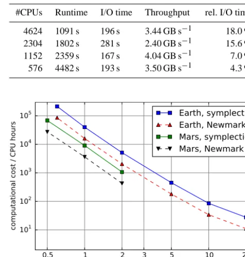
Table 1. I/O performance for a typical setup of AxiSEM on
Super-MUC. The simulation parameters were as follows: 2 s shortest pe-riod, 3600 s simulation length, model: ak135f, vertical component, maximum source depth 700 km. The resulting uncompressed wave field file has a size of 675 GB. The I/O throughput is not affected much by the number of CPUs involved. The throughput between different runs varies, which is probably caused by the changing I/O load on the system.
#CPUs Runtime I/O time Throughput rel. I/O time
4624 1091 s 196 s 3.44 GB s−1 18.0 %
2304 1802 s 281 s 2.40 GB s−1 15.6 %
1152 2359 s 167 s 4.04 GB s−1 7.0 %
576 4482 s 193 s 3.50 GB s−1 4.3 %
0.5 1 2 3 5 10 20
shortest period / s 101
102 103 104 105
computational cost / CPU hours
Earth, symplectic
Earth, Newmark
Mars, symplectic
Mars, Newmark
Figure 15. Computational cost in CPU hours (measured on Monte
Rosa: a Cray XE6 for Earth and Piz Daint, a Cray XC30 for Mars) to generate full Instaseis databases with 1 h long seismograms for two time schemes: 2nd order Newmark and 4th order symplectic.
and spatial sampling have no significant adverse effect on accuracy, i.e. any remaining errors vanish within numerical accuracy of the forward solver AxiSEM.
4.2 Database size
hori-zontal (60 %) components are computed and therefore usable independently.
Several examples are shown in Fig. 14: for Earth, a com-plete reciprocal database including all three components, all epicentral distances and sources down to 700 km and 1 h of seismogram length accurate down to 2 s period, is about 1 TB in size. Calculating such a database once and storing it on a central server will give any user arbitrary and immediate ac-cess to short-period synthetic seismograms without any fur-ther cost. More specialized databases are possible: for exam-ple to study inner core phases for shallow events in an epi-central distance from 140 to 160◦, 200 GB storage suffices to store a database with a frequency of 2 Hz.
4.3 Performance
To evaluate the overall performance of Instaseis, two dis-tinct parts have to be analyzed: first, the databases have to be generated with AxiSEM. Though very efficient, the database generation at short periods is a high-performance computing task. However, AxiSEM scales well on up to 10 000 cores such that global wave fields can be computed at the high-est frequencies within hours on a supercomputer. Detailed performance and scaling tests of AxiSEM can be found in Nissen-Meyer et al. (2014), here we just show the total CPU time required to compute full databases (i.e. horizontal and vertical component) for 1 h long seismograms for two differ-ent time schemes (2nd order Newmark and 4th order sym-plectic Nissen-Meyer et al., 2008) and two planets (Earth and Mars) at a variety of resolutions, see Fig. 15. The gen-eral scaling of AxiSEM is proportional toT−3, whereT is the shortest period resolved by the mesh. The slight discrep-ancy from this power law at longer periods is due to the thin crustal layers causing a smaller global time step in the simu-lation. Simulations for Mars are approximately a factor of 5 faster than for Earth, due to the smaller radius.
The performance of the second part, the seismogram ex-traction, on the other hand is rarely limited by raw comput-ing power. It scales linearly with increascomput-ing frequency of the databases’ Green’s functions and can easily be accomplished on a standard laptop. The limiting factor in most cases is the latency of the storage system, e.g. the time until it starts read-ing from the database. To alleviate this issue we implement a buffering strategy on the functions reading data from the files: the Green’s functions from a whole element of the nu-merical grid are read once and cached in memory. If data from the same element is needed again at a later stage it will already be in memory, thus avoiding repeated disc access. Once the cache memory limit is reached, the data with the earliest last access time is deallocated, effectively resulting in a priority queue sorted by last access time. This optimiza-tion is very effective for most common use cases as they of-tentimes require seismograms in a small range of epicentral distances and depths.
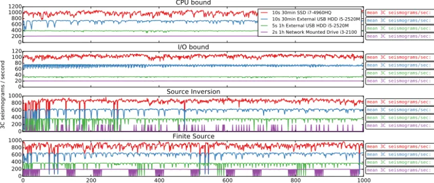
Instaseis comes with a number of integrated benchmarks to judge its performance for a certain database on a given system. The benchmarks emulate the computational require-ments and data access patterns of some typical use cases like finite source simulations and source parameter inversions. Fi-nite sources within the benchmarks are simulated by calcu-lating waveforms for moment tensor sources on an imagi-nary fault plane along the equator ranging from the surface to a depth of 25 km. One source is calculated for each kilo-meter in depth until the bottom of the fault is reached. This is repeated each kilometer along the fault’s surface trajectory until the benchmark terminates. A source parameter inver-sion is simulated by calculating seismograms from moment tensor sources randomly scattered within 50 km distance to a fixed point. Results for four runs are shown in Fig. 16. As is the case with all benchmarks they have to be interpreted carefully, nonetheless they demonstrate the behavior and per-formance characteristics of Instaseis on real machines.
5 Applications
In this section we depict several possible use cases of Insta-seis. This list is not exhaustive and deliberately unconnected to provide a broad overview.
5.1 Graphical user interface
To prominently highlight the features and nearly instanta-neous seismogram extraction for arbitrary source and re-ceiver combinations of Instaseis, we developed a cross-platform graphical user interface (GUI), shown in Fig. 17. It ships with the standard Instaseis package and is written in PyQt, a Python wrapper for the Qt toolkit.
Most evidently, this may be used for visual inspection and verification of any given AxiSEM Green’s function database. Instaseis’ performance permits an immediate visual feed-back to changing parameters. This also delivers quantita-tive insight for an intuiquantita-tive understanding of the features and parameter sensitivities of seismograms. Examples of this are the polarity flips of first arrivals when crossing a mo-ment tensor’s nodal planes, the triplication of phases for shallow sources, the Hilbert transformed shape of reflected phases and the relative amplitude of surface waves (espe-cially overtones) depending on the earthquake depth. Fur-thermore, the GUI allows the calculation of seismograms from finite sources and the exploration of waveform differ-ences in comparison to best-fitting point sources.
5.2 IRIS web-interface
ap-0 200 400 600 800 1000 1200
mean 3C seismograms/sec: 997.8
mean 3C seismograms/sec: 716.0 mean 3C seismograms/sec: 387.3
mean 3C seismograms/sec: 215.6
CPU bound
10s 30min SSD i7-4960HQ 10s 30min External USB HDD i5-2520M 5s 1h External USB HDD i5-2520M 2s 1h Network Mounted Drive i3-2100
0 20
4060
80 100 120
mean 3C seismograms/sec: 103.6
mean 3C seismograms/sec: 72.1 mean 3C seismograms/sec: 34.6
mean 3C seismograms/sec: 20.7
I/O bound
0 200 400 600 800 1000
mean 3C seismograms/sec: 854.5
mean 3C seismograms/sec: 610.8 mean 3C seismograms/sec: 349.6
mean 3C seismograms/sec: 30.2
Source Inversion
0 200 400 600 800 1000
Seismogram Number 0
200 400 600 800 1000
mean 3C seismograms/sec: 873.9
mean 3C seismograms/sec: 625.8 mean 3C seismograms/sec: 348.9
mean 3C seismograms/sec: 179.6
Finite Source
3C seismograms / second
Figure 16. Results of benchmarks for four typical use cases run on different hardware with a variety of shortest periods. The graphs show the
inverse time for the calculation of the ith three-component seismogram. Each run calculated 1000 three-component seismograms, is repeated 10 times with the same random seed, the top and bottom values are discarded, and the mean of the remaining eight values is plotted. The CPU and I/O bound scenarios illustrate the speed with a fully efficient and a deactivated cache, respectively. The two bottom scenarios emulate real use cases, see the main text for details. Amongst other things they show the consequence of a too small cache in the source inversion scenario for the 2 s run and the efficiency of the buffer in the finite source scenario for the same database.
Figure 17. Screenshot of the Instaseis graphical user interface (GUI). Aside from quickly exploring the characteristics of a given Green’s
104 105 106 107 108 109 1010 #Waveforms
10-1 100 101 102 103 104 105 106
CPU time / h
Yspec
WKBJ
Instaseis
Instaseis incl.
DB generation
Figure 18. Computational cost to compute many synthetic
seismo-grams for finite-frequency tomography with a shortest period of 2 s using different methods. For Yspec we assume that for every source there are 1000 receivers with 3 components each. The shaded re-gions for Instaseis indicate the dependence of the performance on the actual source receiver distribution, compare Fig. 16. Including the cost to generate the database with AxiSEM, Instaseis breaks even with Yspec for 14 000 waveforms, which is equivalent to about 5 sources in this configuration.
proach (Tromp et al., 2010), this interface will be able to handle arbitrary sources and receivers independent from cat-alogue data or other parameter limitations. The interface and databases will be described and benchmarked in detail in a separate publication, the status of this project can be viewed on http://ds.iris.edu/ds/products/ondemandsynthetics. 5.3 Finite-frequency tomography
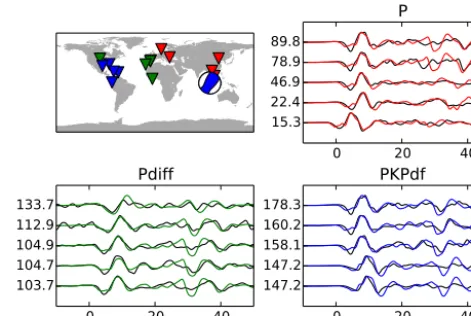
In finite-frequency tomography (e.g. Nolet, 2008) informa-tion is extracted from recorded seismograms by matched fil-ters in multiple frequency bands (Sigloch and Nolet, 2006; Colombi et al., 2014). A matched filter correlates a predicted signal with the measured signal to detect the predicted sig-nal in the presence of noise. In the case of seismic tomog-raphy, a synthetic seismogram is necessary, which is usually created by convolving a Green’s function with an estimated source-time function. For body waves, short periods down to 1 s are commonly used (e.g. Stähler et al., 2012; Hosseini and Sigloch, 2015). Typical data sets contain thousands of earth-quakes (e.g. Auer et al., 2014), each recorded at hundreds of stations, resulting in up to a million waveforms. For each of these waveforms, a separate Green’s function has to be calculated, which requires solving the seismic forward prob-lem at the desired frequencies. For wave propagation meth-ods that solve the forward problem separately for each event, computing these reference synthetics presents a formidable computational challenge, which is why previous studies re-sorted to approximate solutions like WKBJ (Chapman, 1978) or the reflectivity method (Fuchs and Müller, 1971). The full method implemented in Yspec (Al-Attar and Woodhouse,
0 20 40
15.3 22.4 46.9 78.9 89.8
P
0 20 40
103.7 104.7 104.9 112.9 133.7
Pdiff
0 20 40
147.2 147.2 158.1 160.2 178.3
PKPdf
Figure 19. Comparison between observed seismograms (black)
and Instaseis synthetics for the Sumatra earthquake on 30 Septem-ber 2009 with magnitudeMw7.5 at 82 km depth. Vertical axis la-bels are epicentral distances, horizontal is time relative to the ray-theoretical arrivals. A Gabor filter with 3.7 s central period is ap-plied to all traces and the synthetics are convolved with an inverted source time function (Sigloch and Nolet, 2006). The waveforms are aligned by computing relative time-shifts between data and syn-thetic seismograms using cross-correlation (similar to actual finite-frequency tomography).
2008) is about an order of magnitude faster than AxiSEM in computing seismograms for a single source. However, at least in the current implementation, the cost scales linearly with the number of events.
BCIP GRGR MTDJSDDR TGUH HIA
MDJ
ALE
BFO
BORG
CMLA ERM
ESK
KDAK
KWAJ
NNA NRIL
OBN
RPN
SACV IL09
ADK
AFI
BBSR BILL
BOCO DWPF GUMO
HRV KEV
KIP
KNTN
KONO
LCO MA2
MIDW
OTAV PAYG PET
PTCN
PTGA
RAR
RCBR
SAML SFJ
TARA
TBT TIXI
TOL
WAKE
XMAS YAK
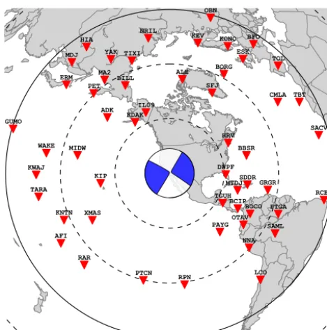
Figure 20. Stations used in the source inversion validation (SIV)
exercise. Circles mark 30, 60 and 90◦epicentral distance. The fi-nite source is aM7.8 strike-slip earthquake in southern California represented by≈105point sources, the beach ball represents the centroid moment tensor, i.e. the orientation and predominant direc-tion of slip of the overall fault.
5.4 Probabilistic source inversion
Uncertainties in source parameters have been shown to have a strong influence on waveform tomography (Valentine and Woodhouse, 2010). Probabilistic point source inversion es-timates the uncertainties of source parameters and their cor-relation. From these, the effect on seismic tomography can be estimated (Stähler and Sigloch, 2014). It requires the re-peated calculation of synthetic waveforms for varying mo-ment tensors, depths and source time functions to calculate the likelihood and posterior probability density of models in a Bayesian sense. Changing source time function and mo-ment tensor is extremely efficient from an Instaseis perspec-tive, and the limitation to a fixed epicenter means that the I/O buffering can be done very efficiently, which is reflected in the Source Inversion test case in the benchmark (Fig. 13).
From a previous study (Stähler and Sigloch, 2014), we assume that for an inversion for depth, the moment tensor and the source time function, a 20-dimensional model space has to be sampled, which requires to perform roughly 60 000 forward simulations. Using 100 seismic stations and three-component seismograms, this means that roughly 1.8·107 waveforms have to be calculated for one source inversion, costing on the order of 50–100 CPU hours (Fig. 18).
5.5 Finite sources
Finite sources can be represented in Instaseis by a cloud of point sources without limitations on the fault geometry or source time functions. Each point source needs to be at-tached with a moment tensor, a slip rate function and a time shift relative to the origin time. These can for instance be retrieved from standard rupture format (*.srf) or subfault format (*.param) files as provided by the USGS for most events withM >6.5. As a show case, we computed the seis-mograms for the source inversion validation (SIV) exercise #3 (http://equake-rc.info). The source is aM7.8 strike-slip earthquake on the San Andreas Fault represented by≈105 point sources, where each source has a different mechanism and slip rate function. The 52 stations are in 30 to 90◦ epi-central distance (see Fig. 20), where the P wave arrival is supposed to be well separated (compare Fig. 1). Excluding the cost of generating the database, it cost a total of 12 CPU hours to compute the 52 1-hour-long three-component seis-mograms accurate down to 5 s.
Figure 21 compares the Instaseis seismograms to P-phases computed with the frequency–wave number integra-tion method (fk) by Kikuchi and Kanamori (1982), where only direct and surface reflected phases where taken into account. While the first arriving waves agree to certain ex-tent with Instaseis providing systematically larger ampli-tudes, there are significant differences for later time win-dows. These are due to additional phase arrivals within the time window (especially triplicated PP, compare Fig. 1) and crustal reverberations not modeled by the fk method. For events with long rupture durations as in this example (200 s) this suggests that more accurate waveforms should be bene-ficial for finite source inversions.
5.6 Insight/Mars
The upcoming NASA-lead Mars Insight mission (Banerdt, 2013), to be launched in March 2016 and scheduled to land September 2016, will deploy a single station with both a broad-band and a short-period seismometer on Mars. This will be the first extra-terrestrial seismic mission since the Apollo lunar landings (1969–1972) and Mars Viking mis-sions (1975) with the goal of elucidating the interior structure of a planet other than Earth. The instrument will record local, regional, and more distant marsquakes (including meteorite impacts) and send data back to Earth for analysis.
cur-0 75 150 time after P / s
DWPF29.82 TGUH 32.25 KDAK 34.74 HRV 35.59 IL09 36.61 MTDJ 37.32 KIP 39.08 BCIP 40.94 PAYG 41.30 SDDR 42.05 BBSR 42.44 ADK 46.90 OTAV 48.19 BOCO 48.28 SFJ 49.93 XMAS 50.01 ALE 52.38 MIDW 52.42
0 75 150
time after P / s
GRGR53.53 BILL 54.81 NNA 58.58 PTCN 60.02 RPN 60.81 PET 61.45 BORG 61.95 PTGA 62.44 MA2 63.34 KNTN 63.89 SAML 65.43 TIXI 65.84 RAR 68.85 WAKE 69.46 CMLA 70.47 YAK 71.15 AFI 71.30 KEV 73.37
0 75 150
time after P / s
TARA 73.73 KWAJ 74.05 ESK 74.32 LCO 75.57 ERM 75.59 NRIL 75.61 KONO 76.66 TBT 80.55 MDJ 82.05 TOL 83.35 SACV 83.57 HIA 83.79 BFO 84.27 RCBR 84.80 OBN 88.38 GUMO 90.18
fk
Instaseis
Figure 21. Seismograms for the SIV benchmark, Z-component aligned on the P arrival band-pass filtered between 5 and 100 s period. The
labels denote the station code and epicentral distance. In the frequency–wave number integration (fk, Kikuchi and Kanamori, 1982), only direct P and the depth phases were included, while Instaseis provides full seismograms, including PP, PcP and other phases. Especially for the stations in less than 40◦distance, the effect is profound, since PP arrives as a triplicated complex wave train only 70–100 s after P. Due to the long source duration, the PP arrival overlaps with the direct P wave train for several stations.
Figure 22. Seismic waves traveling in Mars after a meteorite impact
at its north pole computed with AxiSEM. P-waves are shown in blue and S-waves and surface waves in red.
rent areophysical data (mean mass, mean moment of inertia, tidal Love number, and tidal dissipation) and thermodynamic modeling methods and summarize our current understanding of the internal constitution of the planet. AxiSEM and hence Instaseis can readily be used to propagate waves on Mars, see Fig. 22, allowing us to build these databases very efficiently. 5.7 Synthetic ambient seismic noise
As mentioned in Sect. 2.3, seismograms generated by force sources can be extracted from the same reciprocal databases. This is particularly interesting for studying ambient seismic noise. By cross-correlating noise recorded at two stations, us-ing long enough time series and under certain assumptions (uncorrelated, isotropically distributed white noise sources), it is possible to retrieve the Green’s function of the medium between the two stations (e.g. Sanchez-Sesma, 2006; Goué-dard et al., 2008). However, not all of these assumptions are met in nature, e.g. the noise sources are not evenly distributed (Tsai, 2009; Froment et al., 2010; Basini et al., 2013). Also, the noise sources themselves are not yet well understood, es-pecially with respect to the generation of Love waves in the microseismic band (Nishida et al., 2008).
0.0 1.5 3.0 4.5 6.0 7.5 9.0 10.5 12.0 significant waveheight / m
200 100 0 100 200
time / s
even source distribution
Green's function noise correlation
200 100 0 100 200
time / s
sources only in the oceans, amplitude proportional to significant waveheight (January 3rd 2015) Green's function noise correlation
Figure 23. Synthetic ambient seismic noise cross correlations computed with Instaseis. Left: 100 000 vertical force sources located in the
oceans and amplitude proportional to the significant wave height from the NOAA WAVEWATCH III model on 3 January 2015 (Tolman, 2009). Red crosses indicate the receivers located in Munich and Zurich. Right: cross correlations of 20 days of noise for (top) evenly distributed noise sources and (bottom) the sources in the map, the traces are normalized to their maximum amplitude.
We computed noise cross correlations, accurate down to a period of 5 s, for a total of 20 days of noise data gener-ated with 100 000 noise sources. The calculation only took 1 CPU hour. In the first case, the noise sources consist of vertical forces with a random source-time function, all have the same amplitude and are distributed evenly on the globe. The resulting cross correlation is in good agreement with the Green’s function, which is obtained by introducing an im-pulse source at each of the stations in Zurich and Munich. In the second case, sources are located in the oceans only, their amplitude proportional to the significant wave height (Gualtieri et al., 2013). For the two stations located in Zurich and Munich, the close sources are thus solely located in the west, which leads to strong asymmetry in the retrieved cor-relations (Stehly et al., 2006). Instaseis thus enables users to study noise on the global scale across the microseismic band, by generating realistic waveforms at negligible cost.
6 Conclusions & Outlook
In this paper we presented a readily available methodology and code to extract seismograms for spherical earth mod-els from a Green’s function database. High efficiency in the generation of databases and very fast extraction (on the order of milliseconds per seismogram) of highly accurate seismograms (indistinguishable from conventional forward solvers) can then replace previously employed approxima-tions such as WKBJ, reflectivity or frequency–wave number integration methods that were used for computational rea-sons in many applications of global seismology. Instaseis is open source and available with extensive documentation at www.instaseis.net.
Future developments include Cartesian local domains with layered models, which are not yet supported by AxiSEM. As a large fraction of earthquakes are located below oceans and
receivers on continents, it may be beneficial for body waves studies to take advantage of the axisymmetric capability of AxiSEM and place the receiver on a circular “island” of con-tinental crust within a global oceanic crustal model.
Author contributions. M. van Driel and L. Krischer implemented Instaseis, M. van Driel, S. C. Stähler and T. Nissen-Meyer continu-ously develop AxiSEM and added the database output, and K. Hos-seini prepared the finite-frequency example. M. van Driel prepared the manuscript with contributions from all co-authors.
Acknowledgements. We thank the reviewers C. Tape and D. Al-Attar as well as the editor T. Taira for their constructive comments that helped to substantially improve the manuscript. We thank Alex Hutko and Chad Trabant (IRIS) for valuable discussions on the database selection and implementation as well as user demand. Amir Khan provided the Mars model and Olaf Zielke the reference data used in Fig. 21. Celine Hadziioannou supported us to design the noise example. We gratefully acknowledge support from the European Commission (Marie Curie Actions, ITN QUEST, www.quest-itn.org) and the EU-FP7 VERCE project (no. 283543). Data processing and downloading was done using ObsPy (Megies et al., 2011; Beyreuther et al., 2010) and ObsPyLoad (Scheingraber et al., 2013). Computations were performed at the ETH central HPC cluster (Brutus), the Swiss National Supercomputing Center (CSCS), the UK National Supercomputing Service (HECToR) and the Leibniz Supercomputing Center (LRZ), whose support is gratefully acknowledged.
References
Al-Attar, D. and Woodhouse, J. H.: Calculation of seismic dis-placement fields in self-gravitating earth models – applications of minors vectors and symplectic structure, Geophys. J. Int., 175, 1176–1208, doi:10.1111/j.1365-246X.2008.03961.x, 2008. Astiz, L., Earle, P., and Shearer, P.: Global Stacking of
Broadband Seismograms, Seismol. Res. Lett., 67, 8–18, doi:10.1785/gssrl.67.4.8, 1996.
Auer, L., Boschi, L., Becker, T. W., Nissen-Meyer, T., and Giardini, D.: Savani : A variable resolution whole-mantle model of anisotropic shear velocity variations based on mul-tiple data sets, J. Geophys. Res.-Solid Earth, 119, 3006–3034, doi:10.1002/2013JB010773, 2014.
Banerdt, W.: InSight: A Discovery Mission to Explore the Interior of Mars, 44th Lunar Planet. Sci. Conf., The Woodlands, Texas, 18–22 March 2013, 2013.
Basini, P., Nissen-Meyer, T., Boschi, L., Casarotti, E., Verbeke, J., Schenk, O., and Giardini, D.: The influence of nonuniform ambi-ent noise on crustal tomography in Europe, Geochem. Geophys. Geosys., 14, 1471–1492, doi:10.1002/ggge.20081, 2013. Beyreuther, M., Barsch, R., Krischer, L., Megies, T., Behr, Y., and
Wassermann, J.: ObsPy: A Python Toolbox for Seismology, Seis-mol. Res. Lett., 81, 530–533, doi:10.1785/gssrl.81.3.530, 2010. Burger, W. and Burge, M.: Principles of Digital Image Processing:
Core Algorithms, Springer, London, UK, 2009.
Chapman, C. H.: A new method for computing synthetic seis-mograms, Geophys. J. Int., 54, 481–518, doi:10.1111/j.1365-246X.1978.tb05491.x, 1978.
Colombi, A., Nissen-Meyer, T., Boschi, L., and Giardini, D.: Seis-mic waveform inversion for core-mantle boundary topography, Geophys. J. Int., 198, 55–71, doi:10.1093/gji/ggu112, 2014. Crotwell, H. P., Owens, T. J., and Ritsema, J.: The TauP Toolkit:
Flexible seismic travel-time and ray-path utilities, Seismol. Res. Lett., 70, 154–160, 1999.
Friederich, W. and Dalkolmo, J.: Complete synthetic seismograms for a spherically symmetric earth by a numerical computation of the Green’s function in the frequency domain, Geophys. J. Int., 122, 537–550, doi:10.1111/j.1365-246X.1995.tb07012.x, 1995. Froment, B., Campillo, M., Roux, P., Gouédard, P., Verdel, A., and
Weaver, R. L.: Estimation of the effect of nonisotropically dis-tributed energy on the apparent arrival time in correlations, Geo-physics, 75, SA85–SA93, 2010.
Fuchs, K. and Müller, G.: Computation of synthetic seismograms with the reflectivity method and comparison with observations, Geophys. J. R. Astron. Soc., 23, 417–433, 1971.
Geller, R. J. and Ohminato, T.: Computation of synthetic seismo-grams and their partial derivatives for heterogeneous media with arbitrary natural boundary conditions using the Direct Solution Method, Geophys. J. Int., 116, 421–446, doi:10.1111/j.1365-246X.1994.tb01807.x, 1994.
Gouédard, P., Stehly, L., Brenguier, F., Campillo, M., Colin de Verdière, Y., Larose, E., Margerin, L., Roux, P., Sánchez-Sesma, F. J., Shapiro, N. M., and Weaver, R. L.: Cross-correlation of ran-dom fields: mathematical approach and applications, Geophys. Prospect., 56, 375–393, doi:10.1111/j.1365-2478.2007.00684.x, 2008.
Gualtieri, L., Stutzmann, E., Capdeville, Y., Ardhuin, F., Schimmel, M., Mangeney, A., and Morelli, A.: Modelling secondary
micro-seismic noise by normal mode summation, Geophys. J. Int., 193, 1732–1745, doi:10.1093/gji/ggt090, 2013.
Holtzman, B., Candler, J., Turk, M., and Peter, D.: Seismic Sound Lab: Sights, Sounds and Perception of the Earth as an Acoustic Space, in: Sound, Music Motion, edited by: Aramaki, M., Der-rien, O., Kronland-Martinet, R., and Ystad, S. L., Springer, Mar-seille, France, 161–174, 2013.
Hosseini, K. and Sigloch, K.: Multi-frequency measurements of core-diffracted P-waves (Pdiff) for global waveform tomography, Geophys. J. Int., in review, 2015.
Hua, C.: An inverse transformation for quadrilateral isoparametric elements: analysis and application, Finite Elem. Anal. Des., 7, 159–166, 1990.
Igel, H., Takeuchi, N., Geller, R. J., Megnin, C., Bunge, H.-P., Clévédé, E., Dalkolmo, J., and Romanowicz, B.: The COSY Project: verification of global seismic modeling algo-rithms, Phys. Earth Planet. Inter., 119, 3–23, doi:10.1016/S0031-9201(99)00150-8, 2000.
Kawai, K., Takeuchi, N., and Geller, R. J.: Complete syn-thetic seismograms up to 2 Hz for transversely isotropic spherically symmetric media, Geophys. J. Int., 164, 411–424, doi:10.1111/j.1365-246X.2005.02829.x, 2006.
Khan, A. and Connolly, J. A. D.: Constraining the composition and thermal state of Mars from inversion of geophysical data, J. Geo-phys. Res., 113, E07003, doi:10.1029/2007JE002996, 2008. Kikuchi, M. and Kanamori, H.: Inversion of complex body waves,
Bull. Seismol. Soc. Am., 72, 491–506, 1982.
Komatitsch, D. and Tromp, J.: Spectral-element simulations of global seismic wave propagation-II, three-dimensional models, oceans, rotation and self-gravitation, Geophys. J. Int., 150, 303– 318, doi:10.1046/j.1365-246X.2002.01716.x, 2002a.
Komatitsch, D. and Tromp, J.: Spectral-element simulations of global seismic wave propagation-I. Validation, Geophys. J. Int., 149, 390–412, doi:10.1046/j.1365-246X.2002.01653.x, 2002b. Kristekova, M., Kristek, J., and Moczo, P.: Time-frequency
mis-fit and goodness-of-mis-fit criteria for quantitative comparison of time signals, Geophys. J. Int., 178, 813–825, doi:10.1111/j.1365-246X.2009.04177.x, 2009.
Masson, Y., Cupillard, P., Capdeville, Y., and Romanowicz, B.: On the numerical implementation of time-reversal mirrors for tomographic imaging, Geophys. J. Int., 196, 1580–1599, doi:10.1093/gji/ggt459, 2013.
Megies, T., Beyreuther, M., Barsch, R., Krischer, L., and Wasser-mann, J.: ObsPy – What Can It Do for Data Centers and Observa-tories?, Ann. Geophys., 54, 47–58, doi:10.4401/ag-4838, 2011. Montagner, J. and Kennett, B. L. N.: How to reconcile body-wave
and normal-mode reference earth models, Geophys. J. Int., 125, 229–248, doi:10.1111/j.1365-246X.1996.tb06548.x, 1996. Monteiller, V., Chevrot, S., Komatitsch, D., and Fuji, N.: A hybrid
method to compute short-period synthetic seismograms of tele-seismic body waves in a 3-D regional model, Geophys. J. Int., 192, 230–247, doi:10.1093/gji/ggs006, 2012.
Nishida, K., Kawakatsu, H., Fukao, Y., and Obara, K.: Back-ground Love and Rayleigh waves simultaneously generated at the Pacific Ocean floors, Geophys. Res. Lett., 35, L16307, doi:10.1029/2008GL034753, 2008.
Nissen-Meyer, T., Fournier, A., and Dahlen, F. A.: A two-dimensional spectral-element method for computing spherical-earth seismograms – I. Moment-tensor source, Geophys. J. Int., 168, 1067–1092, doi:10.1111/j.1365-246X.2006.03121.x, 2007b.
Nissen-Meyer, T., Fournier, A., and Dahlen, F. A.: A 2-D spectral-element method for computing spherical-earth seismograms – II. Waves in solid-fluid media, Geophys. J. Int., 174, 873–888, doi:10.1111/j.1365-246X.2008.03813.x, 2008.
Nissen-Meyer, T., van Driel, M., Stähler, S. C., Hosseini, K., Hempel, S., Auer, L., Colombi, A., and Fournier, A.: AxiSEM: broadband 3-D seismic wavefields in axisymmetric media, Solid Earth, 5, 425–445, doi:10.5194/se-5-425-2014, 2014.
Nolet, G.: A Breviary of Seismic Tomography: Imaging the Interior of the Earth and Sun, Cambridge University Press, Cambridge, UK, 2008.
Nyquist, H.: Certain topics in telegraph transmission theory, Trans. AIEE, 617–644, doi:10.1109/5.989875, 1928.
Rew, R. and Davis, G.: NetCDF: an interface for scientific data ac-cess, Comput. Graph. Appl. IEEE, 10, 76–82, 1990.
Sanchez-Sesma, F. J.: Retrieval of the Green’s Function from Cross Correlation: The Canonical Elastic Problem, Bull. Seismol. Soc. Am., 96, 1182–1191, doi:10.1785/0120050181, 2006.
Scheingraber, C., Hosseini, K., Barsch, R., and Sigloch, K.: Ob-sPyLoad: A Tool for Fully Automated Retrieval of Seismo-logical Waveform Data, Seismol. Res. Lett., 84, 525–531, doi:10.1785/0220120103, 2013.
Sigloch, K. and Nolet, G.: Measuring finite-frequency body-wave amplitudes and traveltimes, Geophys. J. Int., 167, 271–287, doi:10.1111/j.1365-246X.2006.03116.x, 2006.
Stähler, S. C. and Sigloch, K.: Fully probabilistic seismic source in-version – Part 1: Efficient parameterisation, Solid Earth, 5, 1055– 1069, doi:10.5194/se-5-1055-2014, 2014.
Stähler, S. C., Sigloch, K., and Nissen-Meyer, T.: Triplicated P-wave measurements for P-waveform tomography of the mantle transition zone, Solid Earth, 3, 339–354, doi:10.5194/se-3-339-2012, 2012.
Stehly, L., Campillo, M., and Shapiro, N. M.: A study of the seis-mic noise from its long-range correlation properties, J. Geophys. Res., 111, B10306, doi:10.1029/2005JB004237, 2006.
Tolman, H.: User manual and system documentation of WAVEWATCH-III version 3.14, Tech. Rep., US Department of Commerce, National Oceanic and Atmospheric Administration, National Weather Service, National Centers for Environmental Prediction, Camp Springs, USA, 276, 2009.
Tromp, J.: Theory and Observations – Forward Modeling and Syn-thetic Seismograms: 3-D Numerical Methods, Treatise on Geo-physics, 2007.
Tromp, J., Komatitsch, D., Hjörleifsdóttir, V., Liu, Q., Zhu, H., Peter, D., Bozdag, E., McRitchie, D., Friberg, P., Trabant, C., and Hutko, A.: Near real-time simulations of global CMT earth-quakes, Geophys. J. Int., 183, 381–389, doi:10.1111/j.1365-246X.2010.04734.x, 2010.
Tsai, V. C.: On establishing the accuracy of noise tomography travel-time measurements in a realistic medium, Geophys. J. Int., 178, 1555–1564, doi:10.1111/j.1365-246X.2009.04239.x, 2009. Valentine, A. P. and Woodhouse, J. H.: Reducing errors in seis-mic tomography: combined inversion for sources and struc-ture, Geophys. J. Int., 180, 847–857, doi:10.1111/j.1365-246X.2009.04452.x, 2010.
van Driel, M. and Nissen-Meyer, T.: Seismic wave propagation in fully anisotropic axisymmetric media, Geophys. J. Int., 199, 880–893, doi:10.1093/gji/ggu269, 2014a.