Control
Vakhtang Rodonaia*Abstract
The new adaptive method of decision making in problems of terminal control is proposed. Unlike the traditional program methods, which are characterized by lack of feedback, the proposed method provides a continuous control over the current state of the controlled object. This requires measurements of controlled variables and corresponding corrections of them to provide the desired development of the terminal control process. The adaptive method is completely described by determining control variables and boundary conditions. Three particular cases met in practice are considered.
Keywords: Decision making, terninal control, variational problem, adaptive control, controlled variables, feedback, boundary condi-tions.
Introduction
In the last years, new problems in automatic control theory arose. Space vehicles, for instance, require minimal fuel consumption or minimal heating during the descent from the orbit and passage through the atmosphere. Such prob-lems as robots’ arms motion control, air traffic control over large airports, soft landing of space satellites, control of physical and technological processes in CAD/CAM sys-tems, animation in computer graphics and many other problems made it extremely significant to focus attention to the methods of terminal control of objects, since these methods allow us to achieve a given phase state of the ob-ject at a given moment of time. In other words, we can, for instance, to move the object to a chosen point of the space with a given velocity vector within the desired time (Batenko A.P.,1977, Milnikov A.A.,2007, 2008).
Basic idea of the terminal control is as follows. Let us consider one-dimensional motion of a controlled object, the coordinate of which is γ. It is obvious that its motion is described by the following system of differential equa-tions.
(1) Where V is the motion velocity of the controlled object under consideration; Fi (i=1, 2, …,n) are the projections of uncontrolled forces on the direction of motion, i.e. on the
y-axis; fj (j = 1, 2, …, k) are the projections of controlled forces on the direction of motion, i.e. on the y-axis; m is the object mass. Uncontrolled forces may include, for ex-ample, all perturbations generated by the environment in which the motion takes place.
The terminal state control problem is formulated as follows. Given the initial phase state of the object y0, 0, it is required to transfer it – within time T - to the terminal state . Uncontrolled forces are functions of time t, the coordinate y and velocity while controlled forces, in addition to being all these functions, are also functions of the controlling parameter
a1 - . Note that the parameter a is
frequently the position of the controlling element and may be a function of time. The traditional approach to the solu-tion of the above-stated mosolu-tion control problems consists in finding the functions for which solu-tions of system (1) satisfy, on the time interval [0; T], the corresponding boundary conditions. The uniqueness of a solution is obtained by using an additional condition re-quiring that solutions must supply an extremum to some specially chosen functional. Such an additional condition is frequently the requirement for a control time minimum (quick action maximum) or an energy minimum of control-ling forces.
Assume that the above said conditions are taken into account in the form:
(2) Where ȹ(t) is some function of controlling forces, kc
- the coefficient of proportionality.
Assume also that a relation between the controlling parameter a(t) and the value of the current (measured) fo rce can be written in the form of an inertia element of first order
1 For example, in the case of jet engines the throttle may play the role of a controlling parameter.
(3)
The control process is therefore described by means of the system of differential equations (1)÷(3). Knowing the synthesized function of controlling forces ȹ(t), we can transfer object from the initial state to the ter-minal state . However, here we encounter a difficulty caused by the necessity to measure controlling forces. This, obviously, can be done if these forces are separated from controlled forces during the object motion. Solutions obtained in this manner are of program charac-ter (the control system is open). Unfortunately, from the practical standpoint, the latter is an unsolvable problem and leads to the instability of the realized motion because of the unforeseen influence of uncontrolled forces. This circumstance requires the development of adaptive meth-ods that demands a different approach: it is necessary to keep a continuous control over the current state of the con-trolled object, which requires respective measurements to be taken. So, the decision about the further development of the process must be made at every step. Here we have to note, that in (Batenko A.P.,1977) it is assumed (without proving) that the control function y(t) can be represented as a certain degree polynomial with unknown coefficients. Unlike, in (Milnikov A.A,2007, V.I. Rodonaia, 2012) we suggested the rigorous formal derivation of the shape for controlled polynomial on the base of solution of a vari-ational problem.
Statement of the Problem
Let us take into account the fact that any change of control-ling forces brings about a change of uncontrolled forces too. All forces (uncontrolled +controlled) acting on the controlled object generate the object motion acceleration . . It is obvious that can be easily measured directly and therefore we should pose the problem on the synthesis of a controlling function in the form of acceleration . Then the control process reduces to the fulfillment of the equality
(4) Where is the measured acceleration of the object and is the given (synthesized) acceleration of the ob-ject.
Note that (4) is actually the equation of motion of the controlled object under the action of the controlling func-tion and is equivalent to (1). This is explained by the fact that the measured acceleration of the object takes into account changes of both uncontrolled and controlled forces
Let us assume that the relation between the given ac-celeration and controlling forces
is
Where k is the proportionality coefficient.
The synthesis of a control algorithm can be reduced to some variational problem in a phase space: given two points and in a two-dimensional phase space, it is required to derive the equation of a curve of this phase space that connects and and delivers a minimum to the next functional
(6) The equation of the curve we want to define can be written parametrically as , . Then it is ob-vious that to the phase curve defined in this manner there corresponds the motion trajectory from the point y0 to the point . The initial velocity at the initial moment of time
t=t0 is equal to ẏ0 and at the terminal moment of time t = T - ẏf
From (6) it follows that the trajectory y=y(t) and delivering a minimum to (6) is optimal in the sense that it minimizes energetic controlling actions.
The acceleration along the optimal trajectory is the function of phase coordinates
(7) From (4) and (5) we have
(8) Substituting (8) into (6) we obtain
(9) Where k1 = 1/k
Functional (9) belongs to the type of functionals that contain derivatives of second order and therefore its cor-responding Euler equation can be written in the form
(10) Solution (10) is a third order polynomial
(11) The boundary conditions are:
particular cases defined by various values of the boundary conditions (12) and (13).
Adaptive Method of Decision Making in Terminal Control Process.
A. Bringing Problem:
First, let us consider the bringing problem. The problem is defined by the following boundary conditions:
(14) (15) Conditions (14) and (15) mean that the object should be transferred from the initial state y=y and to the state and at that, its motion velocity should be arbitrary. For problems of this kind, the given boundary conditions (14) and (15) are supplemented by the so-called natural boundary condition, which in our case looks like (A.E.Bryson,&Ho Yu-Chi, 1969)
(16) Where . After some elemental transformation (V.I. Rodonaia, 2012) we obtain expressions for Ci (i = 0, 1, 2, 3):
(17) Substituting (17) into the first and the second deriva-tive of (11), we obtain the following expressions for an op-timal trajectory in the phase space:
(18)
(19) The acceleration (the second derivative of (18)) has the form:
(20) This is the law of control for the bringing problem. It means that if the acceleration of the controlled object on the time interval [0;T] is assumed to be constant and equal to (20), then at the moment of time t = T its state will sat-isfy the boundary conditions (13). However, this is an open (program) law of control, i.e. the control law without feed-back. Due to the possibility of direct measurements of the acceleration of a controlled object, (19) can be transformed to the control law with feedback (Batenko A.P., 1977). For
this it is enough to assume the initial phase state to be the current one, i.e. to assume y=y and . In that case, the task fulfillment time should be assumed equal to the remaining time T-t. Then (20) takes the form:
(21) From (21) we see that in this case the acceleration that affects the controlled object ceases to be constant and be-comes dependent on the current velocity and coordinate values of the controlled object, i.e. we have the realization of control with feedback.
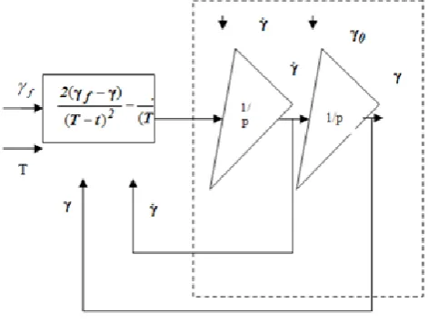
Figure 1 represents the flowchart that implements such a control with feedback. Measured coordinates ( y, ) of the current state enter the block of automatic control sys-tem, where the required value of affecting acceleration is being generated. Thus, here decision on required actions at each step of the control process is made. That is why the method being described is called “adaptive method of decision making.
Figure 1:Control flowchart
B. Acceleration Problem
In the acceleration problem the boundary condition (13) is replaced by
(23) Hence:
(24) (25)
(26)
The last expression is the law of acceleration process control. It means that if on the time interval [0; T] the controlled object is subjected to control (26), then at the moment of time t = T its velocity will satisfy the bound-ary condition (22), i.e. the acceleration problem will be thereby proved.
However, this is again the program law of control and to make it self-correcting (adaptive) we proceed as in the case of the bringing problem, i.e. we replace the initial velocity and coordinate values by the respective current values, and the moment of time T by the difference T - t:
(27)
C. Approach Problem
The approach problem employs four boundary con-ditions (12) and (13) which allow us to calculate imme-diately the coefficients Сi (i=0, 1, 2, 3) in the controlling function (11)
(28) However, frequently it is not enough to have four boundary conditions (12) and (13) to solve the applied problems of terminal control. For example, in the case of deceleration it is not enough to assume that the terminal velocity is equal to zero: for a complete stop it is necessary that the terminal acceleration be equal to zero too. Thus, an additional boundary condition (the fifth one) related to acceleration arises:
(29) It is clear that in this case the controlling function should be taken in the form of a polynomial of fourth order
containing five coefficients, of which only three are to be defined, since it is obvious that the first two coefficients satisfy the first two (initial) conditions (29):
Calculating the first and second derivatives, substitut-ing them into the last three equations (29) and passsubstitut-ing to the control with feedback, we obtain the relevant values of the coefficients Сi (i = 2, 3, 4), y(t),
The adaptive method described above was applied to the problem of spatial rotation of robot manipulator.
Conclusions
• The adaptive method of decision making for terminal control of motion is considered in the paper.
• terminal control methods allow us to achieve a given phase state of the object at a given moment of time
• traditional methods of terminal control have program character (the control system does not have feedback) that leads to the instability of the realized motion due to the unforeseen influence of uncontrolled forces
• adaptive methods (with feedback) must keep a con-tinuous control over the current state of the controlled ob-ject which requires respective measurements to be taken
• decision about the further development of the termi-nal control process (based on measurements taken) must be made at every step.
• in the proposed adaptive methods measured coordi-nates of the current state enter the block of automatic con-trol system, where the required value of affecting accel-eration is being generated. Thus, here decision on required actions at each step of the control process is made.
• the synthesis of a control algorithm can be reduced to variational problem in a phase space
• the adaptive method is completely described by de-termining control variables and boundary conditions
• three particular cases defined by various values of boundary conditions are described
References
Batenko A.P. Control of Terminal States of Moving Objects. Moscow, Sovetskoe Radio, 1977, 225 c. (Батенко А.П. Управление конечным состоянием движущихся объектов. М.: Советское Радио, 1977, 256 с.)
Milnikov A.A., Analysis and Synthesis of Reduction Prob-lem of Terminal Control // ProbProb-lems of Mechanics, Tbilisi, 2008 №1(30), p.67-70
Mechan-ics”, Kutaisi, Georgia, 2007, Vol I, p.17-21
V.I. Rodonaia, “Development of new methods for com-puter modeling of spatial rotation dynamics”, PhD Thesis, Tbilisi, Georgian Technical University, 2012 A.E.Bryson, Ho Yu-Chi, “Applied Optimal Control: