Heuristics Based Tree Switching in Two-sink Sensor Networks

(1)

Heuristics Based Tree Switching in Two-sink Sensor Networks

TEJASMUKESHVASAVADA1

SANJAYSRIVASTAVA2

DA-IICT, Gandhinagar

Abstract. In sensor networks, tree is a well-known topology formation method and TDMA is a desirable MAC protocol due to guaranteed channel access and no collisions. Many times node distribution across the region is not uniform. If finer observations are required in a region, node density is kept high. But in other regions where accurate readings are not needed, network may be sparse. Often multiple sinks are deployed in WSNs. Use of multiple sinks provides fault tolerance and load balancing. When multiple sinks are deployed, more than one sink-rooted trees are formed. The trees with dense node deployment would have higher schedule lengths than the trees with sparse node deployment. Thus trees part of the same network have different schedule lengths. In other words, schedule lengths are not balanced. As a result, nodes of some trees (with higher schedule length) have to wait for longer duration for transmission turn compared to the nodes of the other trees (with lower schedule length). As all the nodes belong to the same network, it is desirable that the waiting time for transmission turn should not be very different. So, schedule length balancing is required to ensure fairness. In this work, an algorithm known as HTSTSN (Heuristics based Tree Switching in Two-sink Sensor Networks) algorithm for two-sink network is proposed. It helps every node to decide which two-sink (i.e. tree) to join such that schedule lengths of trees remain balanced. The HTSTSN algorithm executes before actual scheduling algorithm. It is shown through simulations that the proposed algorithm results in average 13% to 74% reduction in schedule length difference and maximum 12% increase in energy consumption. It is found that the HTSTSN algorithm balances schedule length without much affecting the network lifetime.

Keywords:Sensor Networks, TDMA Scheduling, Multiple sinks, Heterogeneous Networks

(Received November 19th, 2018 / Accepted December 1st, 2019 )

1 Introduction

Sensors are tiny microelectronic devices which can sense physical quantities like temperature, pressure, hu-midity, solar radiation and many others. As mentioned in [1], there are many real life deployments of sensor networks for applications like habitat monitoring, en-vironmental research, volcano monitoring and wild fire detection.

In addition to sensors, sink (also known as base sta-tion) is also deployed in the region. The sink node is connected to the Internet. The sensors send their read-ings to the sink node. The external world can access the readings from the sink.

Once nodes are deployed, logical topology must be

formed so that every node would be able to send its readings towards sink. Tree and cluster are two well-known topology formation methods. We are focused on tree based networks. Sink is the root of the tree. As mentioned in [1], data transfer from sensors to sink is known as convergecast operation.

There are two types of convergecast operations ([1]) : (i) raw convergecast (ii) aggregated convergecast. In raw convergecast, every node forwards all the readings received from children. In aggregated convergecast, ev-ery node aggregates all incoming packets with its own packet and sends out only one packet. We are focused on aggregated convergecast.

(2)

Vasavada et al. Heuristics Based Tree Switching in Two-sink Sensor Networks 2

TDMA (Time Division Multiple Access) and CSMA (Carrier Sense Multiple Access). In TDMA, every node of the tree is assigned time-slot to transmit readings to parent node. As TDMA completely prevents collisions, it is more preferable than CSMA. We have used TDMA in tree-based networks.

If network has to cover large area, large number of nodes need to be deployed. If all the nodes finally join the same tree, the diameter of the tree will increase. In case of aggregated convergecast, increase in tree size will result in increase in schedule length and end-to-end delay. In raw convergecast, funneling effect [1] will also take place.

One solution to reduce the tree size is to deploy more than one sinks. Thus instead of a single large tree, multiple small trees are formed. The schedule length of each small tree would be smaller than that of single large tree.

Sometimes it is required to have accurate readings in some regions of network. In other regions, accuracy may not be needed. To have accurate readings, more sensors are deployed. In the other regions, less sensors are deployed. As a result, some portion of network is dense whereas the other portion is sparse. Thus node distribution is not uniform across the entire network. Many times sensor nodes randomly deployed in the re-gion of interest. When deployment is random, uniform node distribution can not always be guaranteed.

Once nodes are deployed, sink-rooted trees are formed. During tree formation, every node has to join one tree (i.e one sink). If every node joins the sink which is at the smallest hop distance, nodes would be evenly distributed across the sinks. The resulting trees would be of almost equal size and their schedule lengths would be almost same. This happens when node distri-bution is uniform. But when node distridistri-bution is not uniform, the trees would not be of same size if every node decides to join the nearest sink. The trees span-ning dense region of network would have more nodes than the trees spanning through sparse region of the net-work. As a result, the schedule lengths of trees would also be different.

For example, two treesT1andT2 are formed with

schedule lengthsSH1andSH2respectively. The

over-all schedule length SH for the entire network will be max(SH1,SH2). IfSH1 > SH2, SH would be equal

toSH1and vice versa forSH1< SH2.

If schedule length of a tree isSHi, every node of

that tree will get its turn to transmit after SHi

time-slots. Thus ifSH1 > SH2, every node of treeT1will

have to wait for longer duration to get transmission turn compared to the nodes of treeT2. As a result, packets

generated by nodes of treeT1 suffer from longer

end-to-end delay compared to packets generated by nodes ofT2. If schedule lengths are balanced,SH1andSH2

would be almost equal. Thus all the nodes would have to wait for almost equal time to transmit.

If all the nodes are owned by the same user, the nodes and the sinks may co-operate with one another so that both the trees have almost same schedule length. If it is found that one tree is larger than the other tree, nodes from the larger tree may switch to the smaller tree. Accordingly, in this work, an algorithm named as HTSTSN (Heuristics based Tree Switching in Two-sink Sensor Networks) is proposed. The HTSTSN algorithm should run prior to actual scheduling and tree formation algorithm. It guides every node to join a tree such that the resulting trees have balanced schedule lengths. The algorithm is designed for the case that only two sinks are present in the network. It is extensible for more than two sinks.

As summarized in Section II, there are many pa-pers addressing load balancing across multiple sinks for raw convergecast. As per our knowledge, there is no work addressing balancing of schedule lengths of trees in multi- sink aggregated convergecast networks. Our work seems to be only one of its kind.

Rest of the paper is organized as follows: Related Papers are explained in Section II. The Proposed Algo-rithm is presented in Section III. Section IV covers sim-ulation results. Conclusion and Future Work are pre-sented in Section V and VI respectively.

2 Related Work

Some papers addressing issue of tree formation & scheduling in multi-sink sensor networks are summa-rized in this section.

In [7], it is proposed that for each packet sender node should find forward factor for each of the neigh-bors. The forward factor of a node is defined as the ratio of residual energy and distance from sink. The sender node forwards its packet to the neighbor with the high-est forward factor. As residual energy keeps changing, different packets are likely to be sent through different nodes. The nodes with very less energy are not likely to be selected as forwarders. This method indirectly distributes load across sinks as different neighbors are likely to be connected to different sinks.

(3)

The given node may have multiple neighbors through which the selected sink can be reached. For each packet different neighbor is selected probabilistically. As each time different neighbor is selected, workload remains distributed across the neighbors also.

In [9] and [10], it is proposed to change the path towards sink when energy of nodes in the current path goes beyond specific threshold. In [11], the concept of electrical potential field is used to perform load balanc-ing. When a sink finds itself overloaded (i.e. receives too many packets), it informs the nodes in its tree to transmit data to some other sink.

In [12], SMTLB (Spanning Multi Tree Load Bal-anced routing) algorithm is proposed. The aim of the algorithm is to balance the workload across the subtrees of the given tree. Each one hop neighbor of a sink be-comes root of a subtree. The tree is formed in top-down fashion. Different nodes may generate packets at dif-ferent rate. Nodes are gradually added in the subtrees such that total number of packets passing through the subtrees remain almost same.

In [13],tree formation and scheduling are consid-ered as two different problems. It is assumed that more than one sinks are present. Two different methods of tree formation are proposed: (i) In the first method, con-cept of voronoi diagrams is used. Every sink becomes root of exactly one voronoi region. In a given voronoi region, exactly one tree is present. (ii) In the second method, every node is connected to the tree rooted at the sink at smallest hop distance from the given node.

As explained in the previous section, schedule lengths of the trees may not be balanced because of non-uniform node distribution. None of the above men-tioned papers address balancing of schedule lengths in multi-sink tree based networks. Thus it seems that the problem of schedule length balancing must be studied in detail. In [14], core idea of schedule length balanc-ing is proposed without regorous simulations and proof of correctness. The current work is a substantial exten-sion of the work done in [14]. Following are the key differences between the current work and [14].

• In this work, relationship presenting dependenace of schedule length of a tree on node density of the tree and height of the tree is derived empirically. Then it is used for the purpose of shifing nodes from a tree with higher schedule length to a tree with lower schedule length. In [14], shifting of nodes is done but without systematically looking at the relation among schedule length, density of nodes and height of the tree. Thus schedule length estimation and tree switching both are different than in [14].

• Here simulation-based evaluation is more robust than done in [14]. Following points explain the reasons:

– Different sink positions are considered.

– Performance of the proposed algorithm is compared with three other algorithms. In [14], performance is compared with only one trivial algorithm.

– In [14], only performance paramter consid-ered is difference in schedule length. Here, different other parameters like overall sched-ule length, control overhead, energy con-sumption during control phase and energy consumption during data phase are consid-ered.

– In [14], simulation results are presented by just single simulation run for fixed node de-ployment. Here, each performance parame-ter is studied with respect to density denvi-ation of the network for multiple simuldenvi-ation runs with random node deployment.

• The proposed algorithm is supported by the proof of correctness in this work. In [14], correctness of algorithm is not addressed.

Thus our work is a significant extension of the work presented in [14].

3 HTSTSN Algorithm

The HTSTSN algorithm runs before actual scheduling & tree formation algorithm. In [2],[3],[4], DICA([5]) and [6] various scheduling algorithms are proposed. The DICA([5]) seems to be most appropriate approach for scheduling and tree formation in single sink ag-gregated convergecast network due to reason explained next. It follows joint approach i.e. scheduling and tree formation are not dealt separately but considered as a single problem. Every node selects slot and parent at the same time. If tree is formed first and then slot selec-tion is done, the tree structure limits the performance of scheduling algorithm.

A simple extension of DICA([5]) for multiple sinks networks is explained below. It is refered to as hop-count based approach in rest of the paper. It is assumed that number of sinks is two.

(4)

When flooding of HELLO is finished, every node knows its distance in hop count from each sink. Ev-ery node selects the sink at the least hop distance as home-sink. Also for each neighbor, following informa-tion is known: (i) ID of each neighbor (ii) Distance from each sink in hop count (iii) home-sink. Thus every node creates a tablenbr_tableto maintain above mentioned three types of information for each neighbor.

Thus nodes are divided into two different disjoint sets because every node has selected one of the two sinks as home-sink. Now joint scheduling & tree for-mation as proposed in [5] is executed in each group. Every node selects a parent node from the neighbors who belong the same home-sink as the given node. As a result, two different trees are formed and every node is assigned one or more time-slots.

If node distribution is not uniform, the hop-count based approach would results in very different schedule lengths of trees. This is justified through simulation re-sults later. As mentioned earlier, HTSTSN algorithm is proposed in this work to balance the schedule lengths. Detailed discussion of the same algorithm is presented below.

Following are the assumptions used in HTSTSN al-gorithm: (i) There are two sinks in the network. (ii) Every node should be part of exactly one tree. (iii) Ev-ery sink would be root of exactly one tree. (iii) The node distribution may not be uniform.

The HTSTSN algorithm is described considering that two sinks namelyS1andS2are available. But

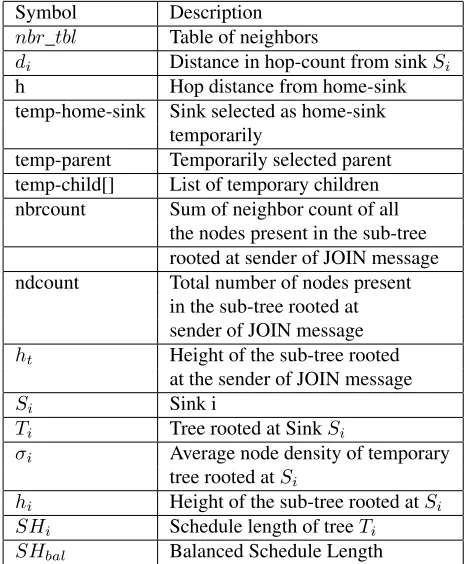
gen-eralized version for the case where number is sinks is more than two is also possible. It is kept as future re-search work. The HTSTSN algorithm has two phases: (i) Estimation of schedule length (ii) Tree Switching Process. During the first phase, every sink estimates the schedule length of its possible tree. In the sec-ond phase, nodes from the tree with higher schedule length are shifted to the tree with lower schedule length. Different notations used in sub-sequent discussion are summarized in Table 1.

3.1 Estimation of Schedule Length

1. The sinksS1andS2 send HELLO packets in the

network one by one. So, every node knowsd1and

d2. The nbr_table is also created.

2. The nearest sink is selected as temp-home-sink. That is, temp-home-sink isS1ifd1= min(d1,d2),

elseS2is temp-home-sink. The heighthof every

node is set to min(d1,d2).

Thus nodes are divided into two different dis-joint sets. First set consists of the nodes who have

Symbol Description

nbr_tbl Table of neighbors

di Distance in hop-count from sinkSi

h Hop distance from home-sink

temp-home-sink Sink selected as home-sink temporarily

temp-parent Temporarily selected parent temp-child[] List of temporary children

nbrcount Sum of neighbor count of all

the nodes present in the sub-tree rooted at sender of JOIN message

ndcount Total number of nodes present

in the sub-tree rooted at sender of JOIN message

ht Height of the sub-tree rooted

at the sender of JOIN message

Si Sink i

Ti Tree rooted at SinkSi

σi Average node density of temporary

tree rooted atSi

hi Height of the sub-tree rooted atSi

SHi Schedule length of treeTi

SHbal Balanced Schedule Length

Table 1: Notations used in HTSTSN Algorithm

selectedS1as temp-home-sink and those who

se-lectedS2are in the second set. Nodes in both the

sets will perform following two steps.

3. Starting from leaf nodes, every node selects one node as temp-parent. The temp-parent is nearer to temp-home-sink compared to the given node. In other words, given node can send packets to its temp-home-sink via temp-parent.

4. Every node sends JOIN message to its temp-parent to inform that it is selected as a parent. The flow of JOIN messages takes place in bottom-up man-ner. That is, it starts from the leaf nodes. Every non-leaf node at heighthsends JOIN message to its parent only after it overhears JOIN from all the nodes at height h+ 1 with respect to the same temp-home-sink.

The fields present in the JOIN message are as follows: nbrcount, ndcount and height ht. The

nbrcount is the sum of neighbors of all the nodes present in the subtree rooted at the sender node. The ndcount is the count of nodes present in the sub-tree rooted the sender node. The heighthtis

(5)

same temp-home-sink as itself while calculating nbrcount and ndcount.

5. Every sinkSi receives JOIN messages from its

children. Every sink Si calculates average node

density (σi) and height of temporary tree (hi). The

average node density (σi) is ratio of sum of

neigh-bors of all the nodes present in the tree and total number of nodes present in the tree. The height of temporary tree is the maximum of heights of its sub-trees.

To study effect of density (σ) and height (h) on schedule length (SH), DICA([5])) is executed for different combinations of σ and h. It is found that following expression represents relationship betweenSH,σandh.

SH= (0.2∗σ∗h) + (0.3∗h) + (2∗σ)−5 (1)

6. Every sink Si estimates SHi using equation 1.

SinkS1sendsSH1toS2and vice versa. Each of

them calculatesSHbal. TheSHbalis an average

ofSH1andSH2.

7. IfSHi > SHbal, following two sub-steps are

per-formed bySi:

(a) The value of hbal is estimated. The value

ofhbalrepresents the required height so that

SHiequalsSHbalfor givenσ. The nodes at

hight greater thanhbalare asked to move to

a different tree.

hbal=

SHbal−(2∗σi) + 5

(0.2∗σi) + (0.3)

(2)

(b) The LOAD_BAL_REQD message is

flooded in the tree rooted at Si. Flooding

is done by Si. Following fields are present

in the message: σ1,σ2,h1,h2,SH1,SH2,

SHbalandhbal.

(c) The nodes receivingLOAD_BAL_REQD message attempt to shift to a different tree using tree switching process described in the next sub-section.

8. If SHi ≤ SHbal, sink Si floods

N O_BAL_REQD message in its tree. Nodes receiving N O_BAL_REQD message under-stand that they need not move to a different tree. They broadcast a message termed as SIN K_CON F IRM ED.

3.2 Tree Switching

Let us assume that S1 floods N O_BAL_REQD

message and S2 floods LOAD_BAL_REQD

mes-sage. Every node present in the tree rooted S2

will receive LOAD_BAL_REQD message. The N O_BAL_REQD message is received by all the nodes in tree ofS1. Consider that a nodenis present

in tree rooted atS2. If its height is less than or equal to

hbal, it would not change the tree. Else it will switch to

a different tree using pseuodo-code mentioned in Algo-rithm 1. The shifting of nodes to treeT1will start from

the boundary separting the two trees and will continue towards the left boundary of the entire area.

At the end, when all the nodes decide their trees (i.e. sinks), joint scheduling & tree formation DICA([5]) is executed for slots and parents selection.

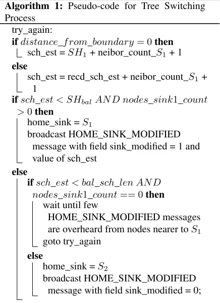
Algorithm 1: Pseudo-code for Tree Switching Process

try_again:

ifdistance_f rom_boundary= 0then sch_est =SH1+ neibor_count_S1+ 1 else

sch_est = recd_sch_est + neibor_count_S1+

1

ifsch_est < SHbalAN D nodes_sink1_count

>0then

home_sink =S1

broadcast HOME_SINK_MODIFIED message with field sink_modified = 1 and value of sch_est

else

ifsch_est < bal_sch_len AN D nodes_sink1_count== 0then

wait until few

HOME_SINK_MODIFIED messages are overheard from nodes nearer toS1

goto try_again

else

home_sink =S2

broadcast HOME_SINK_MODIFIED message with field sink_modified = 0;

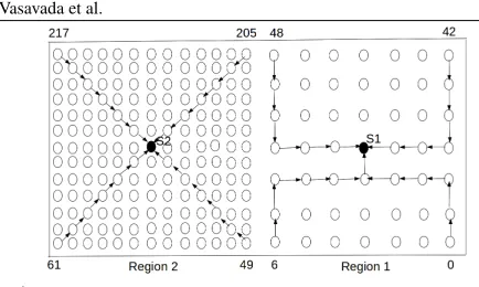
The pseudo-code of Algorithm 1 is explained using Figure 1 in next few paragraphs. In Figure 1, two sinks S1andS2are present. There are total 218 nodes,

(6)

Figure 1: Sample node deployment to illustrate tree switching process

In the figure, sample tentative trees are shown. Not all the edges are shown. The treeT1is made from nodes

of Region 1 and treeT2is made of nodes of Region 2.

The schedule lengths ofT1 andT2 areSH1 andSH2

respectively. As Region 2 is denser than Region 1,SH2

would be higher thanSH1.

SinksS1 andS2 would floodN O_BAL_REQD

and LOAD_BAL_REQD messages respectively in their trees. Every node of Region 1 would broadcast SIN K_CON F IRM EDmessage.

The nodes 49,62,75,88,101,114,127,140,153,166,179, 192 and 205 are at the boundary of Region 1 and 2. So, first if condition would be true for them. They would overhear SIN K_CON F IRM ED message. They are at one hop distance from Region 1. As a result, they will consider schedule length of tree rooted atS1

asSH1. Then each of those nodes would estimate the

resulting schedule length if it would join tree ofS1i.e.

sch_est.

Thesch_estis sum ofSH1,neibor_count_S1and

1. Initially, schedule length of tree rooted atS1isSH1.

Assume that 5 neighbors of given node have switched toS1. Each of them will require one slot to transmit

their packets. So, SH1 should increase by 5. Here

neibor_count_S1 is represents the number of

neigh-bors of given node who have moved toS1. The given

node would require 1 slot to transmit its packet. So, finally ‘1’ is added.

The given node would switch to S1 if the

esti-mated schedule length is less than SHbal and there

is at least one node nearer to S1 in its

neigh-borhood (nodes_sink1_count > 0). This is re-flected in compound condition mentioned in second if in pseudo-code. The node would also broad-cast HOM E_SIN K_M ODIF IED message (with sink_modif ied flag set to 1)to inform its neighbors

that it has changed the tree. If the estimated schedule length is less thanSHbal but there is no node nearer

toS1 is neighborhood, given node would wait for its

neighbors to switch toS1.

If neither the estimated schedule length is less than SHbal nor there is at least one node nearer to S1 in

its neighborhood, node would not switch to a different tree. But it would stick toS2. Still it would

broad-cast HOM E_SIN K_M ODIF IED message (with sink_modif iedflag set to 0) to inform its decision to neighbors.

Nodes of Region 2 other than

62,75,88,101,114,127,140,153,166,179,192 and

205 are not at the boundary i.e. more than

one hop distance from Region 1. They would

not hear SIN K_CON F IRM ED message from nodes of Region 1. But they would hear HOM E_SIN K_M ODIF IED messages from

neighbors. Each HOM E_SIN K_M ODIF IED

message contains new schedule length of tree rooted at S1. Given node waits to receive multiple such

messages. It selects the largest value of new estimated schedule length and assigns to variablerecd_sch_est. The same variable is used to calculatesch_est (else part of first if).

4 Correctness of HTSTSN Algorithm

In this section, various proofs are presented to show that the HTSTSN algorithm works correctly.

Lemma 4.1. In aggregated convergecast, the schedule length (SH) of tree T depends on its average node den-sity (σ) and height (h).

Proof. It is always required that the time-slot assign-ment must be collision-free in nature. That is, when a node transmits a packet in the assigned time-slot, the receiver of the packet should not be receiving or over-hearing from a different node in the same time-slot. As wireless devices are generally half-duplex, the receiver can not even transmit in the same slot.

Let us denote number of neighbours of receiver asx and every node is assigned one slot. When a time-slot is assigned to the transmitter node, the time-time-slot should be different than the slots used by thosex neigh-bors of the receiver. Because if the transmitter transmits to the receiver in any of thosexslots, packets sent from the transmitter would collide with the packets sent by some neighbor of the receiver.

(7)

increase. As every node selects a time-slot consider-ing that collision does not occur at the receiver, dense neighborhood would result in increase of the total slots used to schedule the entire network. That is, the sched-ule length is going to increase.

In aggregated convergecast, it is desired that parent should first receive packets coming from the children. Then send its own packet. This would allow the parent to perform aggregation and send the aggregated packet in the same TDMA cycle with the children. Thus as-signment of time-slot should start from the leaf nodes and progress towards the sink. Suppose, there are p nodes in the path from node to the root,ptime-slots are needed (one for each node). Thus as length of the path increases, the count of slots used to schedule the entire path increases. In other words, number of slots required to schedule a tree depends on height of the tree. The tree height is distance from the farthest leaf.

From above discussion, it can be concluded that in aggregated convergecast network, schedule length de-pends on node density and height of the tree.

Lemma 4.2. The HTSTSN algorithm ensures that when actual trees are formed, every node gets at least one path to the selected home-sink.

Proof. If given node wants to switch to a different home-sinkSi, it would switch if following two

condi-tions are true: (i) The new estimated schedule length of treeTiwould be less than balanced schedule length.

(ii) There is at least one node present in the neighbor-hood of the given node such that the neighbor node has selected sink Si as home-sink and is at a smaller hop

distance from Si compared to the given node. These

two conditions are reflected in if statement as:sch_est < SHbalAN D nodes_sink1_count >0.

If new estimated schedule length is smaller than balanced schedule length but condition (ii) mentioned above is not satisfied, the given node decides not to change its home-sink.

When actual tree formation is initiated by sinkSi,

the given node must have at least one node in neighbor-hood which is part of tree rooted atSiand at a smaller

hop-distance fromSi. So, that node may be selected

as parent. If that potential parent node has selected sinkSias home-sink from begining, it means it has

re-ceived ‘HELLO’ packet from sinkSi. Thus that node

is able to find a path to sinkSi. If potential parent node

has switched to sinkSifrom some other sink, it would

switch only if it has a neighbor which is nearer to sink Si. In any case, sinkSi is reachable through potential

parent. Thus the given node would always find at least

one path to sink Si when actual tree formation takes

place.

Lemma 4.3. The HTSTSN algorithm ensures that when actual trees are formed, their schedule lengths remain balanced.

Proof. As mentioned earlier, if given node wants to switch to a different home-sinkSi, it would switch if

following two conditions are true: (i) The new esti-mated schedule length of tree Ti would be less than

balanced schedule length. (ii) There is at least one node present in the neighborhood of the given node such that the neighbor node has selected sink Si as

home-sink and is at a smaller hop distance from Si

compared to the given node. These two conditions are reflected in if statement as: sch_est < SHbal AN D

nodes_sink1_count >0.

If the given node is just one hop distance from tree Ti, it would useSHito estimate new schedule length

of treeTi. The value ofSHi is calculated by sinkSi

itself based on average node density and height of the tree. To form collision free schedule, number of neigh-bors of the give node already joined treeT1 is added

into SH1. Then finally ‘1’ is added to take into

ac-count transmission slot consumed by the given node. Accordingly, new estimated schedule lengthsch_estis calculated asSH1+ neibor_count_S1 + 1. If it is less

thanSHbal(i.e. average of initial estimate ofSH1and

SH2), node would attempt to switch to treeTi.

If the given node is more than one hop dis-tance from tree Ti, it is likely that some other

nodes around the given node have already switched to tree Ti. When a node switches to a different

tree, it broadcasts SIN K_M ODIF IED message. The message contains new estimated schedule length of that tree. The given node may receive multiple SIN K_M ODIF IED messages. Thus multiple val-ues of new estimated schedule lengths of treeTi. To

be on safer side, node selects the maximum of all the received values as new estimated schedule length of tree Ti. It is denoted as recd_sch_est. Now

neibor_count_S1 + 1 are added in recd_sch_est to

estimate schedule length of treeTi if the given node

joinsTi. If it is less thanSHbal, node would attempt to

switch to treeTi

Thus the given node would switch to new tree only if new estimated schedule length of that tree is smaller thanSHbal. As a result, schedule length of node‘s tree

(8)

Sr. No. p1 p2 σdev

1 0.3 0.3 3

2 0.3 0.5 4

3 0.3 0.7 5

4 0.3 0.9 6

Table 2: Simulation Scenarios

5 Simulation Results

5.1 Simulation Design

All the simulations are performed using Network Sim-ulator 2 (NS-2.35). The nodes are deployed in a region of 200m x 200m like in Figure 1. In Figure 1, node de-ployment is in grid. But for simulations, random node deployment is used. The region is divided into 2000 x 2000 grid points. Any two neighboring horizontal or vertical grid points are at a distance of 10m. There are two sub-regions. Each is of size 100m x 200m.

Node deployment is probabilistic in nature. The probability that a node is present at a grid point in Re-gion 1 (p1) is 0.3 and probability for the same in Region

2 (p2) is varied from 0.3 to 0.9 as shown in Table 2.

In Table 2, four different scenarios are presented. For each scenario, density deviation (σdev) is calculated

as explained next. Consider that there aremnodes in the network. Let σi be the neighbor count of nodei,

then average densityσis defined as follows:

σ=

Pm i=1σi

m (3)

Density deviation (σdev) for the entire network is

calculated as follows:

σdev= r Pm

i=1(σ−σi)∗(σ−σi)

m (4)

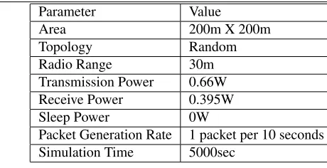
As seen from Table 2, density deviation varies from 3 to 6. From scenario 1 to 4, density of nodes in Re-gion 1 remains fix. But density of nodes in ReRe-gion 2 increases. So, overall density deviation increases from scenario 1 to 4. The performance of the proposed algo-rithm is studied with reference to density deviation. In simulation results, X-axis in graphs is density deviation. Table 3 summarizes various simulation parameters.

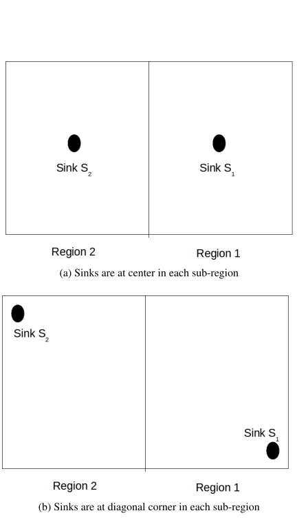
To keep the evaluation robust, three different types of sink placements are used. In Figure 2, sink place-ments are illustrated. In the first case, one sink is present in the center of each region. In the second case, each sink is present at diagonal corner. Lastly, sinks are very near to each other in the third case. Simulation results are generated for each case of sink placement

Parameter Value

Area 200m X 200m

Topology Random

Radio Range 30m

Transmission Power 0.66W

Receive Power 0.395W

Sleep Power 0W

Packet Generation Rate 1 packet per 10 seconds

Simulation Time 5000sec

Table 3: Simulation Parameters

with random deployment of sensor nodes as explained in previous paragraphs.

In graphs, results are plotted against density devia-tion. For every scenario, five different simulation runs are performed. The node deployment is done randomly and varied from one run to other. Each point in graph is an average of values obtain in five different runs. The error bars indicate corresponding standard deviation.

The performance of the HTSTSN algorithm is com-pared with following three different existing algo-rithms.

• Hop count based extension of [5]

• LBR (Load Balanced Routing)[8]

• SMTLB (Spanning Multi Tree Load Balanced routing) [12]

5.2 Performance Measures

Different performance parameters for evaluation of the proposed algorithm are explained in this sub-section. The notations used are as follows: The symbol Ti

means tree spanning Region i. Its schedule length is denoted asSHi. The density of nodes of Region i is

denoted asσi. Total number of sensor nodes is denoted

asm.

• Percentage Difference in Schedule Length (SHdif f) : It indicates the gap betweenSH1and

SH2. It is defined as follows:

SHdif f =

|SH1−SH2|

maximum(SH1, SH2) ∗100

• Maximum Schedule Length (SH) : It is overall schedule length of the network. It is defined as follows:

(9)

(a) Sinks are at center in each sub-region

(b) Sinks are at diagonal corner in each sub-region

(c) Sinks are nearby

Figure 2: Deployment of Sinks

• Control Overhead (CO): It is total number of packets generated during control phase. It is the duration from network initialization till beginning of data transfer. It involves tasks like sending of HELLO packets, packets required for load balanc-ing and schedulbalanc-ing & tree formation.

• Energy Consumption During Control Phase (Eccons): It is average energy consumed per node

due to transfer of control packets by node. It is measured in mJ (milli Joules). Let initial energy of all nodes beEinit. At the end of control phase,

residual energy in node i beEcresii. Average

en-ergy consumption(Eccons)during control phase is

defined as follows:

Eccons= Pm

i=1Einit−Ecresii

m

• Energy Consumption During Data Phase (Edcons):

It is energy consumed due to transfer of data pack-ets. It is also measure in mJ (milli Joules). At the end of control phase, residual energy in node i be Ecresii. At the end of data phase, residual energy

in node i beEdresii Average energy consumption

(Edcons)during data phase is defined as follows:

Edcons= Pm

i=1Ecresii−Edresii

m

The HTSTSN algorithm is compared with hop-count based approach, LBR algorithm and SMTLB al-gorithm. The SMTLB algorithm is a centralized algo-rithm. It is implemented as a C language program by us. Only tree formation and slot assignment are im-plemented for SMTLB. So, density difference, sched-ule length difference and maximum schedsched-ule length are calculated for SMTLB. As control and data packets are not generated, remaining performance measures are not derived for SMTLB algorithm.

5.3 Results & Discussion

In this sub-section, simulation results and related anal-ysis is presented.

5.3.1 Schedule Length Difference

(10)

Figure 3: Dependency of Fractional difference in Schedule Lengths on Density Deviation

Density Deviation (σdev)

Sink Positions 3 4 5 6

Center 26 55 35 36

Diagonal 46 74 13 39

Nearby 40 47 52 40

Table 4: Percentage Improvement in Schedule Length Difference

Increase in density deviation means increase in density of nodes in Region 2, but density of nodes in Region 1 is constant. Thus increase in density deviation results in increase in node density of treeT2compared to that

of treeT1. As a result, SH2 increases without much

change inSH1. Thus, difference in schedule length

in-creases.

The HTSTSN algorithm results in the least schdule length difference between the two trees. In HTSTSN, nodes move from treeT2to treeT1until their estimated

schedule lengths become balanced. So, the difference betweenSH1andSH2is also reduced.

The average percentage improvement in schedule length difference achieved by HTSTSN algorithm is summarized in Table 4. The improvement is calcu-lated with reference to the second best performing al-gorithm. Here the second best performing algorithm is ‘hop-count’ in all three cases i.e. sinks in center, sinks at diagonal corners and sinks nearby. The percentage improvement ranges between 26% to 74%.

The other three algorithms do not perform as good as HTSTSN algorithm due to reasons explained in next few paragraphs.

The SMTLB algorithm is aimed at balancing work-load of sub-trees. We have two sinksS1 andS2.

As-suming that sinkS1hasxnext-hop neighbors and sink

S2hasynext-hop neighbors. As the first step,x

neigh-bors will select sinkS1as parent andyneighbors will

select sinkS2as parent. Thus totalx+ysub-trees are

initiated.

It is considered in SMTLB that different nodes have different workloads i.e. number of packets generated by the node per second. The algorithm progresses in top-down fashion. That is, the sub-trees grow gradu-ally from sink to leaf nodes. The sub-tree with the least work-load is expanded first. The workload of a subtree is the sum to packets generated by all the nodes part of that sub-tree. From the available nodes in range, the node with the least workload is selected to join the sub-tree under consideration.

(11)

de-ployments, Region 2 has higher node density than Re-gion 1. We have assumed that all the nodes have the same workload. So, here total workload of a sub-tree is the total number of nodes part of the sub-tree. As the sub-trees expand in top-down fashion (i.e from sink to leaf nodes), not all the nodes have option to join any of the two sub-trees. The nodes nearer to sinkS1join the

least loaded sub-tree of S1. The nodes nearer to sink

S2join the least loaded sub-tree ofS2. Only the nodes

arond the boundary of the two regions may have sub-trees of bothS1andS2available. As a result, not many

nodes of Region 2 join the tree rooted atS1. As a result,

treeT2has large number of nodes and it is denser than

treeT1. So,SH2remains higher thanSH1. Thus the

schedule length difference in SMTLB remains higher than HTSTSN algorithm.

The parent selection in hop-count based approach takes place based on distance from the sink node. That is, given node joins the tree rooted at the sink at the least hop-distance. All the nodes of Region 2 join treeT2and

nodes of Region 1 join treeT1. As explained earlier, as

treeT2is denser than treeT1,SH2remains higher than

SH1. So, the schedule difference in hop-count based

approach remains higher than HTSTSN algorithm. In LBR algorithm, for each sinkSi, given node finds

the ratio ‘ri’ of number of neighbor nodes of the sink

and hop distance between given node and sinkSi. The

given node joins the tree Ti rooted at the sinkSi for

whom the ration ‘ri’ is maximum. As Region 2 has

denser node deployment than Region 1, most of the nodes of Region 2 join treeT2. Only those nodes of

Region 2 which are far from sinkS2such thatr2> r1,

join treeT1. As very few nodes of Region 2 join tree

T1,SH2 remains higher thanSH1. Thus, LBR

algo-rithm also is not able to reduce the difference between schedule lengths.

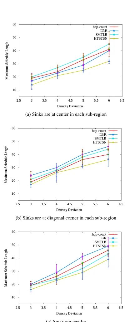
5.3.2 Maximum Schedule Length

The graphs of Max. Schedule Length v/s. Density De-viation are shown in the Figure 4. As defined earlier, maximum schedule length is max(SH1,SH2). The

HT-STSN algorithm results in the least schedule length dif-ference compared to the other three algorithms. As a re-sult, the maximum schedule length as achieved by HT-STSN algorithm is the least. In our simulation setup, SH2>SH1. As in HTSTSN algorithm, nodes of tree

T2switch to treeT1,SH2goes down andSH1goes up.

ButSH1does not increase beyond average of original

values ofSH1 andSH2. Thus max(SH1,SH2) goes

down.

The maximum schedule length increses with in-crease in density deviation. It is explained earlier how

(12)

Center 17 9 18 20

Diagonal 10 23 13 20

Nearby 16 14 14 24

Table 5: Percentage Improvement in Maximum Sched-ule Length

the schedule length difference increases with increase in density deviation. The maximum schedule length is max(SH1,SH2). In our simulation setup, increase in

density deviation means increase in density of nodes in Region 2. That is, increase inSH2. AsSH2increases,

value of max(SH1,SH2) also increases.

The average percentage improvent in maximum schedule length achieved by HTSTSN algorithm is summarized in Table 5. The improvement is calcuated with reference to the second best performing algorithm. The second best performing algorithm is LBR when sinks are in center, SMTLB when sinks are at diago-nal corner and hop-count based approach when sinks are nearby.

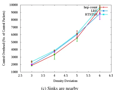
5.3.3 Control Overhead

In Figure 5, graphs of Control Overhead v/s. Density Deviation are presented. It is seen from the graphs that HTSTSN algorithm results in higher control overhead than the other two algorithms. As SMTLB is imple-mented as a stand-alone application program (control and data packets are not simulated), its control overhead is not calculated.

The HTSTSN algorithm uses control messages for three different objectives: (i) estimation of schedule length of each tree (ii) shifting of nodes from one tree to the other (iii) selection of slot and parent. The other two algorithms use control messages only for selection of slot and parent. As HTSTSN algorithm uses more num-ber of control messages, its control overhead is higher than the other algorithms.

The control overhead increases with increase in den-sity deviation. As explained earlier, increase in denden-sity deviation means increase in density of Region 2. Thus number of nodes in tree T2 increases with increase in

density deviation. As number of nodes increases, the number of required slots also increases. So, the control overhead for slot and parent selection also increases. Thus with increase in density deviation, control over-head increases.

(13)

Center 10 9 7 3

Diagonal 12 10 6 4

Nearby 10 11 5 3

Table 6: Percentage Increase in Energy Consumption during Control Phase

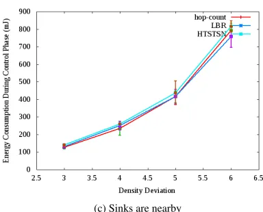
5.3.4 Energy Consumption during Control Interval

In Figure 6, the graphs for Energy Consumption during Control Interval v/s. Density Deviation are presented. The average energy consumed by nodes during control interval is directly proportional to the control messages exchanged i.e. control overhead. The nature of graphs in Figure 6 is same as in Figure 5. So, more explanation is not given.

The control phase in TDMA-based tree networks does not take place too often. The control phase takes place just after network deployment so that logical topology can be formed. Then data transfer phase takes place. In the data transfer phase, sensed readings are transferred to the sink. When there is a considerable change in the topology (i.e. many nodes are deleted or new nodes are added), tree and schedule maintenance is required. Thus control phase takes place again. Thus as control phase does not takes place very frequently, the related energy consumption also does not put much burden on the nodes.

The average percentage increase in control energy consumption suffered by HTSTSN algorithm is sum-marized in Table 6. The difference is calculated with reference to the best performing algorithm which is hop-count based approach in all three cases. It is seen from Table 6 that maximum increase in energy con-sumption is by 12%.

5.3.5 Energy Consumption during Data Interval

The energy consumption during Data Interval remains the same in all the three algorithms. So, corresponding graphs are not shown. All the nodes transmit the pack-ets at the same (1 packet every 10 seconds). In all the three algorithms (i.e. hop-count, LBR and HTSTSN), one hop neighborhood of every node remains the same. So, average number of children per node also remains the same in all the four algorithms. The network is as-sumed to use aggregated convergecast.

Thus as every node transmits 1 packet per 10 sec-onds and number of packets received are also almost same in all the three algorithms, the energy consumed

(14)

during data transmission phase is same in all the three algorithms. Of course, it increases as density deviation increases because, as network becomes denser, aver-age number of neighbors increases. Thus node receives more packets. So, more energy is consumed in packet reception. But for specific value of density deviation, all the three algorithms result in the same data energy consumption.

6 Conclusion

In this work, problem of scheduling & tree formation in the case of two-sink sensor networks is examined. When nodes are not deployed in a uniform manner across the area, some regions have higher node density compared to the other regions. As a result, the trees of dense regions have higher schedule length than the trees passing through the sparse regions. If schedule length of a tree is large, every node of that tree has to wait for long time to get its transmission turn.

We have proposed an algorithm termed as HTSTSN (Heuristics based Tree Switching in Two-sink Sensor Networks) to ensure that the two sink-rooted trees have almost equal schedule lengths. Thus all the nodes of the network wait for almost the same time to get transmis-sion opportunity.

The performance of the HTSTSN algorithm is eval-uated by varying density deviation of the network. It is found that the HTSTSN algorithm results in smaller schedule length difference and smaller maxi-mum schedule length. It results in around 10% higher control energy consumption. But as control phase does not take place frequently, this additional energy con-sumption can be accepted because of advantages like reduction in schedule length difference and maximum schedule length. If sensor nodes are deployed in a re-gion where enough sun-light is available, solar energy may be used instead of traditional battery. In that case, this extra energy consumption may not be an issue at all. The energy consumption during data interval re-mains the same for all the three algorithms.

Thus it can be concluded that the proposed HT-STSN algorithm results in reduction in overall schedule length and schedule length difference between the trees without affecting the network lifetime much.

References

[1] F.Wang et. al, “Networked Wireless Data Col-lection: Issues, Challenges and Approaches", in

IEEE Communication Surveys & Tutorials, Vol. 13, No. 4, 2011.

[2] Ichrak Amdouni et. al, “Joint Routing and STDMA-based Scheduling to Minimize Delays in Grid Wireless Sensor Networks",A Research Re-port, September 2014.

[3] Fang-Jing Wu et. al, “Distributed Wake Up Scheduling for Data Collection in Tree based Wireless Sensor Networks", inIEEE Communica-tion Letters, Vol. 13, Issue 3, 2009.

[4] Chansu Yu et. al, “Many to One Communica-tion Protocol for Wireless Sensor Networks", in

International Journal of Sensor Networks, Inder-science Publications, Vol. 12, Issue 3, 2012.

[5] M.Bagga et. al, “Distributed Low Latency Data Aggregation Scheduling in Wireless Sensor Net-works", in ACM Transactions on Sensor Net-works, Vol. 11, No. 3, April 2015.

[6] M. Wafa et. al,“Energy-Efficient Scheduling in WMSNs",INFOCOMP Journal of Computer Sci-ence, Vol. 8, Issue 1, p. 45-54, March 2009.

[7] C.Wang et. al, “A Load Balanced Routing Algo-rithm for Multi Sink Wireless Sensor Network", inIEEE International Conference on Communi-cation Software and Networks (ICCSN), 2009.

[8] C. Zhang et. al, “Load-balancing Routing for Wireless Sensor Networks with Multiple Sinks", in12th IEEE International Conference on Fuzzy Systems and Knowledge Discovery (FSKD), 2015.

[9] A.N.Eghbali et. al, “An Energy Efficient Load-balanced Multi-Sink Routing Protocol for Wire-less Sensor Networks", in10th IEEE International Conference on Telecommunications, 2009.

[10] H. Jiang et. al, “Energy optimized routing algo-rithm in Multi sink wireless sensor networks", in

International Journal of Applied Mathematics and Information Sciences, Vol. 8, No. 1, 2014.

[11] C. Wu et. al, “A Novel Load Balanced and Life-time Maximization Routing Protocol in Wireless Sensor Networks", inIEEE Vehicular Technology Conference, Spring 2008.

(15)

[13] B. Yu et. al, “Minimum Time Aggregation Scheduling in Multi-Sink Sensor Networks", in

8th Annual IEEE Communications Society Con-ference on Sensor, Mesh and Ad hoc Communica-tions and Networks, 2011.