Paper 05-2008

UDC: 539.374:004.021

Stress Integration for the Drucker-Prager Material Model Without

Hardening Using the Incremental Plasticity Theory

D. Rakić1_{, M. Živković}2_{, R. Slavković}3_{, M. Kojić} 4,5,6

1 _{Faculty of Mechanical Engineering, University of Kragujevac} [email protected]

2 _{[email protected]} 3 [email protected]

4 _{Harvard School of Public Health, Boston, USA} [email protected]

5 _{Research and Development Center for Bioengineering ‘BIOIRC’, Kragujevac, Serbia}

6 _{Department of Biomedical Engineering, University of Texas Medical Center at Houston, USA}

Abstract

This paper presents the formulation of the stress integration procedure for the Drucker-Prager material model with associative yielding condition by using the incremental plasticity theory. The idea of this method is to reach the solution by calculating the plastic matrix according to the method of incremental plasticity (used for elastic matrix corrections), and with use of the total strain increment. The computational procedure is implemented within the program package PAK. Results of this procedure were compared with the solutions obtained by the governing parameter method (Kojic and Bathe 2005), as well as with the results obtained by the program package NX-Nastran.

Keywords: Drucker-Prager model, FEM, Geomechanics, Incremental plasticity

1. Introduction

Stress integration represents calculation of stress change during an incremental step, corresponding to strain increments in the step. It is in essence the incremental integration of inelastic constitutive relationships to trace the history of material deformation. The stress integration is an important ingredient in the overall finite element inelastic analysis of structures. It is important that the integration algorithm accurately reproduces the material behavior since the mechanical response of the entire structure is directly dependent on this accuracy. The algorithm should be also computationally efficient because the stress integration is performed at all integration points. For general applications, this computational procedure should be robust, providing reliable results under all possible loading (straining) conditions (see e.g. discussion of these issues in e.g. Kojic and Bathe 2005).

scheme termed as the governing parameter method (Kojic, 1996), as well as with results obtained by using other software packages.

In the next section we present formulation the Drucker-Prager material model, followed by the derivation of the elastic-plastic constitutive matrix in general associated plasticity. Then, the general relations are implemented on of the Drucker-Prager material model.

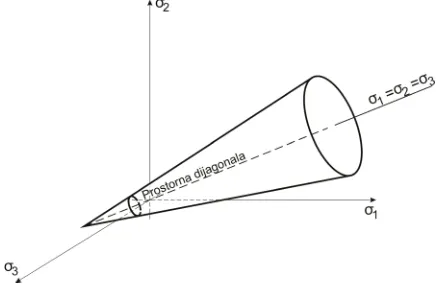
2. Formulation of the Drucker-Prager model

This material model is defined by the yield surface called the Drucker-Prager yield surface. In the space of main stresses, this surface represents a cone, whose axis matches the space diagonal of the coordinate system of principal stresses σ σ σ1, 2, 3 (Figure 1). This material

model is a special case of the Drucker-Prager material model with a cap (Kojic and Bathe 2005).

Fig. 1. Drucker-Prager failure surface.

The model can be represented in the I1− J2D coordinate system, as shown in Fig. 2, where

Fig. 2. Drucker-Prager model in space I₁− J_2D .

1 3 m ij ij ii

I = σ =σ δ =σ (1)

2

1 2

D ij ij

J = S S (2)

is the second invariant of the deviatoric stress. Deviatoric stress S_ij is defined as:

ij ij m ij

S =σ −σ δ (3)

The elastic domain is bounded by the Drucker-Prager surface and by the maximum tension line – with the tension cutoff stress T. This representation of the model is suitable for development of the computational procedure.

If the stress point of a trial solution is above the Drucker-Prager line, the stresses at the end of step have to be reduced to satisfy the following yield condition:

1 2 0

t t t t t t

DP D

f α I J k

+Δ ₌ +Δ ₊ +Δ _{− = (4)}

where α and k are material constants; and the upper left index t+ Δt denotes the end of step. If the stress exceeds the allowed tension stress value, the stress reduction is performed by equalizing all three components of normal stress to one third of the maximum tension stress, i. e.:

11 22 33 ₃

T

σ =σ =σ = (5)

while the shear stress components are set to zero:

0

ij i j

σ = ≠ (6)

3. Elastic-plastic matrix

For an elastic-plastic material, the stress increment

{ }

dσ can be expressed by the total strain increment

{ }

de as

{ }

_{dσ ⎡C}EP_⎤

{ }

_de

= ⎣ ⎦ (7)

where _⎡CEP_⎤

⎣ ⎦ is the elastic-plastic constitutive matrix defined below.

In the case of small strain material deformation, the total strain increment can be divided into elastic and plastic part:

{ }

_{de =}

{ } { }

_deE _{+ de}P ₍₈₎

from which follows

{ }

_deE ₌

{ }

_{de −}

{ }

_deP ₍₉₎

The stress and elastic strain increments are related by the elastic constitutive law,

{ }

_{dσ ⎡C}E_⎤

{ }

_deE

= ⎣ ⎦ (10)

where _⎡CE_⎤

{ }

_{dσ =⎡C}E_⎤

(

{ }

_{de −}

{ }

_deP

)

⎣ ⎦ (11)

We next include into this derivation a yield function F, which in general has a form:

( )

( ij)

F =F σ ≡F σ (12)

A differential of the yield the function can be expressed as

xx yy zz xy yz zx

xx yy zz xy yz zx

F F F F F F

dF dσ dσ dσ dσ dσ dσ

σ σ σ σ σ σ

∂ ∂ ∂ ∂ ∂ ∂

= + + + + +

∂ ∂ ∂ ∂ ∂ ∂ (13)

or in matrix form,

{ }

T

F dF dσ

σ

∂ ⎧ ⎫ = ⎨_∂ ⎬

⎩ ⎭ (14)

In the incremental theory of plasticity we have that the yield function during plastic deformation must be equal to zero (when F≤0 we have elastic unloading), hence F=0 and consequently

0

dF= is satisfied over the load step. The last condition can be written in the following form:

{ }

0

T

F dF dσ

σ

∂ ⎧ ⎫

=_{⎨ ⎬} =

∂

⎩ ⎭ (15)

where T

F

σ ∂ ⎧ ⎫ ⎨ ⎬

∂ ⎩ ⎭ is

T

xx yy zz xy yz zx

F F F F F F F

σ σ σ σ σ σ σ

⎡ ⎤

∂ ∂ ∂ ∂ ∂ ∂ ∂

⎧ _{⎫ = ⎢}

⎥ ⎨ ⎬

∂ ∂ ∂ ∂ ∂ ∂ ∂

⎩ ⎭ ⎢_⎣ ⎥_⎦ (16)

whereas

{ }

dσ is

{ }

dσ = ⎣⎡dσxx dσyy dσzz dσxy dσyz dσzx⎤⎦ (17)

Further, we assume a non-associative plasticity, therefore the increment of plastic strain is

{ }

_deP _dλ G

σ

∂ ⎧ ⎫

= _{⎨ ⎬}

∂

⎩ ⎭ (18)

where:G

( )

σ is the plastic potential function, and dλis a positive scalar.

Substituting the plastic strain increment (18) into (11), we obtain the stress increment:

{ }

_{dσ C}E

{ }

_{de dλ C}E G

σ

∂ ⎧ ⎫

⎡ ⎤ ⎡ ⎤

=_{⎣ ⎦} − _{⎣ ⎦ ∂⎨ ⎬}

⎩ ⎭ (19)

Now, we substitute this stress increment into (15):

{ }

0

T

E E

F G

dF C de dλ C

σ σ

∂ ⎛ ∂ ⎞

⎧ ⎫ _{⎡ ⎤ ⎡ ⎤}⎧ ⎫

=_{⎨ ⎬ ⎜⎣ ⎦} − _{⎣ ⎦⎨ ⎬⎟}=

∂ ∂

⎩ ⎭ ⎝ ⎩ ⎭⎠ (20)

{ }

0

T T

E E

F F G

dF C de dλ C

σ σ σ

∂ ∂ ∂

⎧ ⎫ _{⎡ ⎤} ⎧ ⎫ _{⎡ ⎤}⎧ ⎫

=_{⎨ ⎬ ⎣ ⎦} − _{⎨ ⎬ ⎣ ⎦⎨ ⎬}=

∂ ∂ ∂

⎩ ⎭ ⎩ ⎭ ⎩ ⎭ (21)

Then, the parameter dλ is

{ }

T

E

T E

F _{C de}

d

F _C G

σ λ σ σ ∂ ⎧ _{⎫ ⎡ ⎤} ⎨_{∂ ⎬ ⎣ ⎦} ⎩ ⎭ = ∂ ∂ ⎧ ⎫ _{⎡ ⎤}⎧ ⎫ ⎨_∂ ⎬ _{⎣ ⎦}⎨_∂ ⎬ ⎩ ⎭ ⎩ ⎭ (22)

Finally, substituting dλ from (22) into (19), obtain the relationship between

{ }

dσ and the total strain increment

{ }

de :

{ }

{ }

{ }

T E E E T E G F

C C de

d C de

F _C G

σ σ σ σ σ ∂ ∂ ⎧ ⎫⎧ ⎫ ⎡ ⎤_{⎨ ⎬⎨ ⎬} ⎡ ⎤ ⎣ ⎦_{⎩∂ ⎭⎩∂ ⎭} ⎣ ⎦ ⎡ ⎤ =_{⎣ ⎦} − ∂ ∂ ⎧ ⎫ _{⎡ ⎤}⎧ ⎫ ⎨_∂ ⎬ _{⎣ ⎦}⎨_∂ ⎬ ⎩ ⎭ ⎩ ⎭ (23)

By comparing this and equation (7) it follows:

T E E EP E T E G F C C C C F G C σ σ σ σ ∂ ∂ ⎧ ⎫⎧ ⎫ ⎡ ⎤_{⎨ ⎬⎨ ⎬} ⎡ ⎤ ⎣ ⎦_{⎩∂ ⎭⎩∂ ⎭} ⎣ ⎦ ⎡ ⎤ ⎡= ⎤− ⎣ ⎦ ⎣ ⎦ _{∂ ∂} ⎧ ⎫ _{⎡ ⎤}⎧ ⎫ ⎨_∂ ⎬ _{⎣ ⎦}⎨_∂ ⎬ ⎩ ⎭ ⎩ ⎭ (24)

This is a general expression for the elastic-plastic constitutive matrix. Also, by substituting (22) into (18) we can calculate the plastic strain increment

{ }

_deP _:

{ }

{ }

T E P T E G F C de de

F _C G

σ σ σ σ ∂ ∂ ⎧ ⎫⎧ ⎫ ⎡ _{⎤ ⎨ ⎬⎨ ⎬} ⎣ _{⎦ ∂⎩ ⎭⎩∂ ⎭} = ∂ ∂ ⎧ ⎫ _{⎡ ⎤}⎧ ⎫ ⎨_∂ ⎬ _{⎣ ⎦}⎨_∂ ⎬ ⎩ ⎭ ⎩ ⎭ (25)

In the case of associative plasticity the yield function F is at the same time the plastic potential function. In our implementation of the above general expressions to the Drucker-Prager model we will adopt the associative plasticity assumption.

4. Implementation of the general associative plasticity relations to the Drucker-Prager material model

We further use the Drucker-Prager yielding surface defined as:

1 2D

F =αI + J −k (26)

1 2

dil D

G=α I + J −k (27)

The first invariant I1 is defined by equation (1), while the second stress invariant J2D is defined by (2):

(

) (

2

) (

2

)

2 2 2 2

2 1 2 2 3 3 1 4 5 6

1 6 D

J = ⎡_⎣σ σ− + σ −σ + σ σ− ⎤_⎦+σ +σ +σ (28)

where the one-index notation is used (as in the subsequent text). Also, we can express J_2D as

2

2 2 1

1 3 D

J =I − I (29)

where the second stress invariant I2 is:

2 2 2

2 1 2 2 3 3 1 4 5 6

I =σ σ +σ σ +σ σ σ− −σ −σ (30)

Most frequently used material constants of geological materials (which are experimentally evaluated) are the internal friction angle φ and the cohesion c. They are the

characteristic of the Mohr-Coulomb material model. There are direct relations between these parameters and parameters k and α of the Ducker-Prager model:

(

2sin

)

3 3 sin φ α

φ

=

−

(

)

6 cos 3 3 sin

c

k φ

φ

=

− (31)

These relations are obtained by coinciding the Drucker-Prager cone with the outer apexes of the Mohr-Coulomb hexagon locus (compressive cone).

The derivatives of the Drucker-Prager yield function with respect to stresses can be calculated by using the chain rule:

1 2

1 2

T T

T

D

D

I J

F F F

I J

σ σ σ

∂ ∂

∂ ∂ ⎧ ⎫ ∂ ⎧ ⎫

⎧ _{⎫ = +}

⎨_∂ ⎬ _∂ ⎨_∂ ⎬ _∂ ⎨ _∂ ⎬

⎩ ⎭ ⎩ ⎭ ⎩ ⎭ (32)

Note that this expression is applicable to all models where the yield function is expressed in terms the stress invariants I1 and J2D (which is the case for a large number of plasticity models). Also we have the following relations from (26):

1

F I α

∂ =

∂ (33)

and

2 2

1 2

D D

F

J J

∂ =

∂ (34)

The derivatives of the stress invariants with respect to stresses are:

[

]

1 _{1 1 1 0 0 0}

T

I σ

∂ ⎧ _{⎫ =} ⎨ ⎬

∂

⎩ ⎭ (35)

(

)

(

)

(

)

2

1 2 2 1 2 3 1 2 3 4 5 6

1 ₂ 1 ₂ 1 _{2 2 2 2}

3 3 3

T D

J _{σ σ σ σ σ σ σ σ σ σ σ σ}

σ

∂

⎧ ⎫ ₌⎡ _{− − − + − − − +} ⎤

⎨ _∂ ⎬ _{⎢ ⎥}

⎣ ⎦

⎩ ⎭ (36)

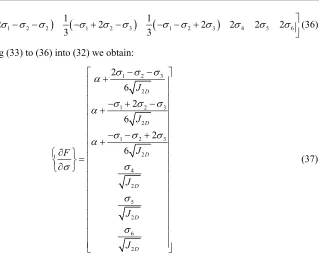
Now, substituting (33) to (36) into (32) we obtain:

1 2 3

2

1 2 3

2

1 2 3

2 4 2 5 2 6 2 2 6 2 6 2 6 D D D D D D J J J F J J J σ σ σ α σ σ σ α σ σ σ α σ σ σ σ − − ⎡ ₊ ⎤ ⎢ ⎥ ⎢ ⎥ ⎢ _{− + −} ⎥ + ⎢ ⎥ ⎢ ⎥ ⎢ _{− − +} ⎥ ⎢ ₊ ⎥ ⎢ ⎥ ∂ ⎧ _{⎫ ⎢= ⎥} ⎨_∂ ⎬ ⎢ ⎥ ⎩ ⎭ ⎢ ⎥ ⎢ ⎥ ⎢ ⎥ ⎢ ⎥ ⎢ ⎥ ⎢ ⎥ ⎢ ⎥ ⎢ ⎥ ⎣ ⎦ (37)

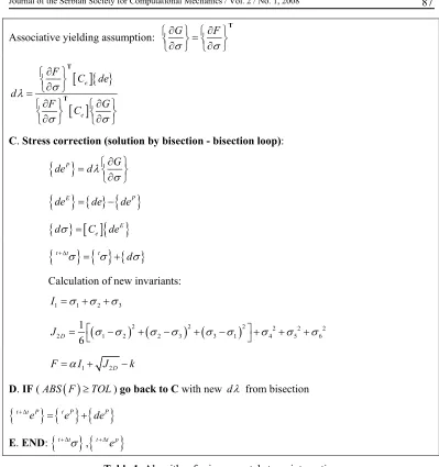
The above relations for the stress integration over a load (time) step are summarized in Table 1. The left upper indices t and t+ Δt denote start and end of a time step.

Known quantities:

{ }

t+Δt_{e ,}

{ }

t_{e ,}

{ }

t_{σ ,}

{ }

t p_e

A. Trial (elastic) results:

{ }

[ ]

{ }

E

[ ]

(

{ } { }

t t t

)

e e

dσ ₌ C de ₌ C +Δe ₋ e

{ } { }

t+Δt_{σ =} t_{σ +}

{ }

_dσ

1 1 2 3

I =σ σ+ +σ

(

) (

2

) (

2

)

2 2 2 2

2 1 2 2 3 3 1 4 5 6

1 6 D

J ₌ ⎡σ σ_{− +} σ ₋σ ₊ σ ₋σ ⎤₊σ ₊σ ₊σ

⎣ ⎦

1 2D

F=αI + J −k

B. Yielding condition check:

IF (F<0) trial result correct (go to E) IF (F≥0) elastic-plastic result (CONTINUE)

1 2

1 2

D

D

I J

F F F

Associative yielding assumption: G F

σ σ

∂ ∂

⎧ ⎫ ⎧₌ ⎫ ⎨_∂ ⎬ ⎨_∂ ⎬

⎩ ⎭ ⎩ ⎭

T

[ ]

{ }

[ ]

e

e

F _{C de}

d

F _C G

σ λ

σ σ

∂ ⎧ ⎫ ⎨_∂ ⎬ ⎩ ⎭ =

∂ ∂

⎧ ⎫ ⎧ ⎫

⎨_∂ ⎬ ⎨_∂ ⎬

⎩ ⎭ ⎩ ⎭

T

T

C. Stress correction (solution by bisection - bisection loop):

{ }

_deP _dλ G

σ

∂ ⎧ ⎫

= ⎨ ⎬

∂ ⎩ ⎭

{ }

_deE ₌

{ }

_{de −}

{ }

_deP

{ }

[ ]

{ }

E e

dσ = C de

{ } { }

t+Δt_{σ =} t_{σ +}

{ }

_dσ

Calculation of new invariants:

1 1 2 3

I =σ σ+ +σ

(

) (

2

) (

2

)

2 2 2 2

2 1 2 2 3 3 1 4 5 6

1 6 D

J ₌ ⎡σ σ_{− +} σ ₋σ ₊ σ ₋σ ⎤₊σ ₊σ ₊σ

⎣ ⎦

1 2D

F=αI + J −k

D. IF (ABS F

( )

≥TOL) go back to C with new dλ from bisection

{

t+Δt P_e

} { } { }

₌ t P_{e + de}P

E. END:

{ }

t+Δt_{σ ,}

{

t+Δt p_e

}

Table 1. Algorithm for incremental stress integration

5. Verification of the computational procedure

Verification of the proposed computational procedure was done by solving elastic-plastic deformation of a sand box specimen, as specified in the literature (Kojic and Bathe 2005).

Fig. 3. Sand specimen – geometry, material data and load.

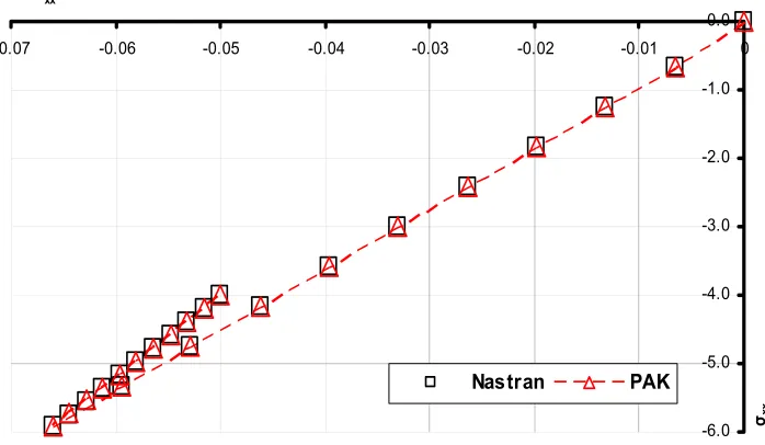
The problem was solved using the program package PAK (Kojic et al. 1998), by employing the described method and the governing parameter method. Also the program NX NASTRAN was used. Figures 4 and 5 show the results.

-6.0 -5.0 -4.0 -3.0 -2.0 -1.0 0.0

-0.07 -0.06 -0.05 -0.04 -0.03 -0.02 -0.01 0

exx

σxx

Nastran PAK

Fig. 4. The calculated axial stress as a function of the axial strain.

Material data:

Young’s modulus, E=100

Poisson’s ratio, ν =0.3

Yield function parameter, α=0.05

Yield function parameter, k=0.1

Tension Cutoff limit, T =0.01

Dimension, D=1.0

Dimension, H =0.5

[1] step [2] displacement u [3] 0 [4] 0.0

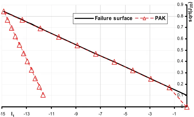
0 0.1 0.2 0.3 0.4 0.5 0.6 0.7 0.8 0.9

-15 I1 -13 -11 -9 -7 -5 -3 -1

s

q

rt(J

2D

)

Failure surface PAK

Fig. 5. The second invariant deviatoric stress as function of first stress invariant. It can be seen from the presented results that all three solutions are practically the same.

6. Conclusions

The presented methodology gives very accurate results when compared with other methods, such as the governing parameter method. The advantage of the presented computational procedure is that it is formulated in general form so that it can be applied to various yield functions. Also, this procedure can be implemented in an explicit computationally efficient incremental scheme, where yield condition check D (Table 1) is not performed, but then very small load steps are necessary.

References

Bathe K. J. (1982), Finite Element Procedures in Engineering Analysis, Prentice-Hall, Inc., Englewood Cliffs, New Jersey.

Geo-Slope Office (2002), Sigma W-for finite element stress and deformation analysis V5, User’s guide.

Kojic M. (1996), The governing parameter method for implicit integration of viscoplastic constitutive relations for isotropic and orthotropic metals, Computational Mechanics, Vol. 19, No. 1, pp. 49-57.

Kojic M., Bathe K. J. (2005), Inelastic Analysis of Solids and Structures, Springer Berlin Heidelberg New York.

Kojic M., Slavkovic R., Zivkovic M., Grujovic N. (1998), PAK-finite element program for linear and nonlinear structural analysis and heat transfer, Faculty for Mechanical Engineering, Kragujevac, University of Kragujevac.