Forestry & Natural-Resource Sciences Last Correction: Feb.20, 2014
ADJACENCY CONSTRAINTS IN FORESTRY – A SIMULATED
ANNEALING APPROACH COMPARING DIFFERENT
CANDIDATE SOLUTION GENERATORS
Paulo Borges, Even Bergseng, Tron Eid
Department of Ecology and Natural Resource Management, Norwegian University of Life Sciences
Abstract. Adjacency constraints along with harvest volume constraints are important in long term
forest management planning. Simulated annealing (SA) has previously been successfully applied when addressing such constraints. The objective of this paper is to assess the performance of SA using three methods for generating candidate solutions. Biased probabilities in the management unit (MU) selection were introduced, one static and one dynamic. The first one (Method 1) is the conventional (static) method. The two other methods were implemented through a search vector used in the candidate solution generator. These methods are based on (Method 2) the number of treatment schedules and standard deviation of NPV within MUs and (Method 3) the MU’s potential improvement in the objective function value, the number of URM adjacency violations an MU is involved in, the period specific volume harvested in an MU and the number of times an MU is selected. The methods were tested on a large number of datasets including 300 hypothetical forest landscapes characterized by three different initial age class distributions, respectively young, normal and old. Evaluation of the methods was accomplished by means of objective function values and first feasible iteration. Solutions improved when introducing bias in the probabilities for MU selection (Methods 2 and 3) compared to the conventional method (Method 1) and when the probability bias for selecting MUs is dynamic (Method 3) rather than static (Methods 1 and 2). The mean improvement for the average GAP obtained by Method 3 for young, normal and old forest landscapes was 20.88%, 12.84% and 5.20%, respectively. Whereas for the minimum GAP the mean improvement was 21.96%, 14.30% and 6.05% for young, normal and old forest landscapes, respectively.
Keywords: OR in Natural Resources; static and dynamic search vectors; grid landscapes; heuris-tics; Unit restriction model.
1
Introduction
Since simulated annealing (SA) was introduced by Kirk-patrick et al. (1983) as a technique for solving opti-mization problems, many disciplines such as biology, telecommunications, geology, electronics and medicine have been using SA as a tool to provide good (eventu-ally optimal) solutions (see e.g. Chibante, 2010). Also in the forestry sector there are numerous optimization problems that can benefit from the use of heuristics like SA. Forestry planning problems include optimization of long term forest plans with detailed information about where, when and how silvicultural treatments should oc-cur (i.e. treatment schedule), transportation of various forest products (e.g. roundwood, forest residuals) to and
from the industry, and optimization of complicated in-dustrial processes.
Over time, long term forestry optimization problems have become more complex since not only the economic aspects are important but also because environmental and social aspects of forestry have received increased attention. This development inevitably has an effect on the development of long term forest planning and its complexity. Accordingly, the dependency on math-ematical programming and information technology has also increased considerably. A typical example would be maximization of economic income over time, under temporal and spatial (adjacency) restrictions. One im-portant aspect of long term forest planning is spatial considerations, typically imposed in order to preserve wildlife habitats or enhance scenic beauty. Such
erations restrict harvesting of neighboring management units (MU, i.e. forest stands) in the same or consecutive time periods.
A lot of work has been done related to adjacency con-straints in long term forest planning (see e.g. reviews of Baskent and Keles, 2005; Weintraub and Murray, 2006; Shan et al., 2009). Adjacency constraints, as defined by Murray (1999), are divided into the unit restriction model (URM), where clear cut is not allowed in neigh-boring MUs in the same time period, and the area re-striction model (ARM), where the total area of neigh-boring MUs harvested in the same time period should not exceed a defined maximum. In addition, the concept of “green-up constraints” is introduced in order to guar-antee a time buffer between two consecutive clear cuts. This concept can be used along with the URM and ARM approaches (e.g. Brumelle et al., 1998; Boston and Bet-tinger, 1999, 2006; McDill et al., 2002 ; Goycoolea et al., 2009; Strimbu et al., 2010). Also the “core area” concept has become important in long term forest plan-ning for example due to conservation of wildlife habitats, where the formation of contiguous areas of old growth forest over time in a forest landscape is promoted (e.g.
¨
Ohman and Eriksson, 1998; ¨Ohman, 2000; Rebain and McDill, 2003).
SA has been successfully applied in many forestry problems addressing adjacency constraints. Like other heuristic methods, SA is based on a neighborhood so-lution search approach. A broad definition of a neigh-borhood of a solution is “the set of solutions which dif-fer slightly from the original one”. In forestry planning applications with adjacency constraints, the neighbor-hood for S-metaheuristics such as simulated annealing and tabu search is usually defined by the set of new so-lutions that can be obtained or reached through a change in timing of clearcut harvests or a change in the applica-tion of management regimes (e.g. Lockwood and Moore, 1993; Boston and Bettinger, 1999; ¨Ohman and Eriksson, 2002; Bettinger et al., 2002; ¨Ohman and L¨am˚as, 2005; Liu et al., 2006; Bettinger and Kim, 2008; Borges et al., 2014).
Another important aspect, along with the neighbor-hood definition, is the candidate solution generator. The solution generator, among the set of neighboring solu-tions selects the one(s) that should be evaluated. In forestry applications, the common procedure when gen-erating a candidate solution is first to assume a uniform probability distribution when selecting an MU, and then within that MU, another uniform probability distribu-tion is applied to select either the period where the clear cut should occur or which treatment schedule to apply. The candidate solution generator, however, can be ma-nipulated in order to improve the quality of solutions (e.g. better objective function values) of the adopted
heuristic (e.g. Borges et al., 2014). This may be done by introducing a bias in the probability distribution for selection of MUs and even treatment schedules. Biased selection criteria in this context means that we are using a probability distribution which is not uniform.
Some previous studies have implemented biased ap-proaches in the MU selection. O’ Hara et al. (1989) used a heuristic that moved only through the feasible space, and three approaches with biased MU selection were compared with an unbiased (uniform) selection ap-proach. The biased approaches were based on the im-provement of the objective function value (harvested vol-ume) and on the fewest effective adjacent units, i.e. the number of new units that cannot be harvested. Barrett and Gilless (2000) implemented bias in the MU selec-tion by sorting the MUs in descending order according the MUs total net present value (NPV) and NPV per ha.
Biased criteria have been applied also in SA forestry applications. For example, ¨Ohman and Eriksson (1998) applied SA maintaining the selection of MUs by first assuming a uniform probability distribution. However, after the MU selection only three treatment schedules among 14 were possible to select, i.e. two treatment schedules moving the period for clear cut one period forward or backward, respectively, and one treatment schedule maintaining the selected MU un-harvested over the entire time horizon. Baskent and Jordan (2002) maintained the selection of MUs by first assuming a uni-form probability distribution, but the final harvest was assigned to the period that returned the lowest harvested volume in order to favor non-violation of the minimum harvest volume constraints. Borges et al. (2014) devel-oped three biased approaches in the MU selection and compared them with the conventional approach where a uniform probability distribution in the MU and treat-ment schedule selection was assumed. The three biased criteria introduced in the MU selection took into account the number of treatment schedules and/or the standard deviation of the NPV within an MU. The biased cri-teria in that study, however, were defined beforehand, i.e. the probabilities of selecting an MU were calcu-lated before the candidate solution generator started and remained constant throughout all SA iterations. This means that the candidate solution generator worked with static search vectors.
ac-count the number of feasible treatment schedules for the MUs.
SA is in general suitable for working in large neigh-borhood frameworks. This is particularly important in forestry problems with adjacency constraints. SA is fairly simple to implement and since it works with two solutions (current and candidate), it is relatively fast when evaluating many solutions. We are not aware of any previous work in the long term forestry planning lit-erature that uses SA where the candidate solution gener-ator applies dynamic probabilities for the MUs selection. The objective of this paper is therefore to assess the per-formance of SA under three different methods for gener-ating candidate solutions. We perform a study where we applied two static search vectors with and without bias and a dynamic search vector with bias. The methods are applied to a large number of randomly generated forest landscapes.
The remainder of this paper is as follows: section 2 de-scribes the general planning model, the case study based on a forestry problem, the simulated annealing approach including the methods for applying the candidate solu-tion generator and finally the measures for how the three methods are compared. Section 3 presents results, sec-tion 4 contains a discussion on how the methods perform, whereas section 5 presents the conclusions.
2
Material and Methods
2.1 General model We use a standard formulation of a forestry planning problem where one treatment schedule is selected for each MUs so that the NPV is maximized over an infinite time horizon. This objective is restricted to the URM adjacency constraints and the sequential flow constraints regarding volume harvested (VH). The mathematical formulation of the problem is as follows:
MAX N P V (1)
Subject to
N P V =X
i∈N
X
k∈T Si
Aipikyik (2)
X
k∈T Si
yik= 1,∀i∈N (3)
X
i∈c
xit≤1,∀c∈C,∀t∈ {1, ..., T} (4)
X
k∈Xit
yik=xit,∀i∈N,∀t∈ {1, ..., T} (5)
V Ht=
X
i∈N
X
k∈T Si
Aiviktyik,∀t∈ {1, ..., T} (6)
0.9·V Ht≤V Ht+1≤1.1·V Ht,∀t∈ {1, ..., T −1} (7)
yik∈ {0,1},∀i∈N, k∈T Si (8)
whereN is the number of MUs,TSiis the set of treat-ment schedules within MUi,T is the number of planning
periods,Xitis the set of treatment schedules of MUithat
produce a clear cut in periodt, C is the set containing all maximal cliques related to the forest graph, i.e. a graph formed by MUs (nodes) and edges that represent the neighboring relation between MUs (see e.g. Murray and Church, 1996a, 1996b; Vielma et al., 2007), Ai is the area of MUi,pik is the NPV per ha associated with
MUi when treated with treatment schedule k, VHt is
the total volume harvested in period t, vik t is the
vol-ume harvested per ha in period t in MUi in treatment
schedulek.
The decision variables yik takes the value 1 if
treat-ment schedulek is applied to MUi, and the value 0
oth-erwise. The decision variable xit takes the value 1 if
MUi is clear cut in periodt, and the value 0 otherwise.
Thus, equation (1) defines the objective function which maximizes NPV, equation (2) defines NPV, equations (3) and (??) secure that only one treatment schedule is applied per MU, i.e. all the area of an MU should be manage by only one treatment schedule, equations (4) and (8) secure that only one MU within a clique can be harvested in each time period, i.e. they define the clique URM adjacency constraints, equation (5) relates the de-cision variablesyikandxit, equation (6) defines the total volume harvested in each time period, inequalities (7) define a 10% allowed variation in flow of the harvested volume between consecutive periods. Note that equa-tion 5 forces the variables xit to be either zero or one,
depending if a treatment schedule (yik) from the setXit
is selected or not respectively. Thus, there is no need to force these variables to be binary.
The problem presented is the same as in Borges et al. (2014) but the formulation of the model is different. Rather than defining the URM adjacency constraints in a pairwise approach, we use the clique approach (e.g. Murray and Church, 1996b). For that, the additional decision variables xit need to be defined and related to the decision variablesyik(equation 5). This formulation is more compact than the formulation made by Borges et al. (2014), i.e. the total number of constraints (4) and (5) are less than the number of constraints needed to define the adjacency constraints in a pairwise approach.
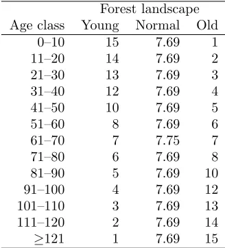
represent three different forest landscapes with different initial age class distributions, namely young, normal and old (Table 1). Each dataset within a forest landscape encompasses 1,600 MUs distributed over a grid of 40 x 40 cells. An area of 1 ha was assigned to all cells. The grid configuration and the equal area assigned to each cell avoid effects of MU size and number of neighbors per MU when assessing the methods. Moreover, the datasets used in this work, are based on 8990 sample plots from the Norwegian national forest inventory (NFI).
Table 1: Age class distribution (%) for the different for-est landscapes.
Forest landscape Age class Young Normal Old
0–10 15 7.69 1
11–20 14 7.69 2
21–30 13 7.69 3
31–40 12 7.69 4
41–50 10 7.69 5
51–60 8 7.69 6
61–70 7 7.75 7
71–80 6 7.69 8
81–90 5 7.69 10
91–100 4 7.69 12
101–110 3 7.69 13
111–120 2 7.69 14
≥121 1 7.69 15
The growth simulator GAYA (Hoen and Eid, 1990; Gobakken, 2003) was applied to generate treatment schedules for the MUs representing the landscapes. The simulator takes as input a set of MUs (plots) and a set of rules which define how and when forest treatments may be applied. The output provides detailed informa-tion on common forest state variables (e.g. standing vol-ume, harvested volume) as well as treatments (e.g. final harvest, thinning) and corresponding economic values ??(incomes and costs) for each treatment schedule for all periods. In addition, NPV is computed based on an infi-nite planning horizon (soil expectation value is included in the NPV) provided for each treatment schedule. In the present study, the following treatments were allowed; natural regeneration and planting, pre-commercial thin-ning, conventional thinning and final harvest (clear cut and seed tree cutting). This means that not only clear cut contributes to the volume harvested in a period but also conventional thinning and seed tree establishment. This means that more harvesting methods are included compared to most previous works (see e.g. Murray and Church, 1996; MacDill and Braze, 2000; Bettinger et al., 2002; Boston and Bettinger, 2006) Moreover, only clear
cut is relevant for the adjacency constraint, as opposed to seed tree cutting where some trees are left for regen-eration proposes. Simulations were performed for ten 10-year periods. A 3% discount rate was applied.
The total number of treatment schedules among the 300 datasets varied between 131,102 and 156,963 corre-sponding to an average of 82 and 98 treatment schedules per MU, respectively. Moreover, within a dataset the minimum number of treatment schedules for MUs was 1 and the maximum varied between 594 and 833.
2.3 Simulated Annealing SA is a meta-heuristic that establishes a relationship between the annealing of solids and optimization problems (Dowsland, 1995). The usual parameters in SA applications are the initial temperature, the number of iterations allowed at each temperature, the cooling rate, and the final temperature at which the search is finished (e.g. Bettinger and Kim, 2008). The solutions producing improvements in the ob-jective function value are always accepted. In order to prevent the search to be trapped in local optima, solu-tions with poorer objective function values can also be accepted depending on a probabilistic threshold which is defined by the current temperature and the differ-ence between the current and candidate solution values. The temperature is kept constant for a certain number of iterations and then gradually reduced, lowering the probability of accepting solutions with poorer objective function values. The candidate solutions are generated based on the current solution, and the search process usually finishes when certain criteria are fulfilled, typi-cally when reaching the final temperature or after per-forming a certain number of iterations.
When applying heuristics, procedures for local search are typically used and a definition of the neighborhood is thus required. Two main approaches can be used. The first one is accepting only feasible solutions within the neighborhood (e.g. Murray and Church, 1995; Liu et al., 2006; O’Hara et al., 1989). However, this approach is costly in terms of computational time, since each new solution needs to be assessed in terms of feasibility (Liu et al., 2006). The second approach is considering infeasi-ble solutions within the neighborhood (e.g. ¨Ohman and Eriksson, 1998; Falc˜ao and Borges, 2001, 2002; Borges et al., 2014). The use of this approach implies some relaxation of the problem, i.e. some constraints are in-cluded in the objective function as penalties in order to worsen the objective function value of solutions that do not satisfy the constraints. In this way, more movements will be considered feasible and less check of feasibility is needed (Liu et al., 2006). This approach is usually faster in terms of computational time.
are penalized more than small ones. However, to con-struct and interpret penalty functions is a difficult task (Falc˜ao and Borges, 2001). Penalty functions should be calibrated properly to ensure convergence towards fea-sible solutions (Lockwood and Moore, 1993). Moreover, according to Lockwood and Moore (1993), the magni-tude of the values of the penalty functions should also be close to the objective function values to secure that none of the components of the new objective function have influence over the others. The resulting evaluation function is usually named “fitness function” and the re-spective value in SA is named “energy”.
In addition, the quality of the solutions obtained de-pends on the SA parameter settings and on the penalty function(s) (if adopted). Therefore, several test runs are required to find suitable values for the parameters. Usu-ally some values for each parameter are tested and the combination producing the best results is adopted. In the present study SA was implemented and each forest landscape was parameterized as described by Borges et al. (2014). This means that the neighborhood definition and parameters setting were the same for all datasets within each forest landscape. In detail, the starting tem-perature was set according to the following formula:
st=−p1×(N P V0) ln(p2)
where,NPV0is the NPV from the initial solution pro-duced by SA,p1is a percentage of the initial NPV value andp2is the probability to accept a solution that varies (worse value) the previous amount. For our datasets we setp1= 1% for all forest landscapes andp2=10 %, 20% and 1% for young, normal and old forest landscapes, re-spectively. For all datasets, the cooling rate was set to 0.995, the number of iterations at each temperature was set to 5,000 and the neighborhood structure was defined by changing one treatment schedule of a selected MU at each iteration (typically called 1-opt moves). Thus, the assessment of solution feasibility is only dependent on the evaluation of URM and sequential flow constraints. As mention, when using the first approach (above) usu-ally, as an SA search matures, a large number of un-successful moves are attempted and rejected (due to vi-olations of constraints or due to severe changes in the objective function value). If the first approach is em-ployed, a process for reducing the temperature every x number of unsuccessful iterations is needed in order for the process to properly terminate. Thus, we decide for the second approach, i.e. accepting infeasible solutions regarding these two types of constraints but penalizing them in the objective function.
Rather than using the penalty function formula ap-plied by Borges et al. (2014), we use a slightly different one where the component penalizing the violation of the
adjacency constraints have been changed. The main rea-son for the modification has to do with the fact that for some runs of SA the last feasible solution reported was found relatively far from the end of the SA run. This will “deteriorate” the values obtained not only for the average but also for the standard deviation of the so-lution values. In Borges et al. (2014), the adjacency constraints were penalized by considering the product between the average NPV per MU and the total number of conflicts among the MUs at the power of two. How-ever, in a situation where only one conflict is observed the total NPV associated with the two MUs that are in conflict can be larger than the respective penalty value if the total NPV associated with the MUs is larger than the average NPV per MU. Therefore, we introduce as penalty value for adjacency constraints, the sum prod-uct between the number of conflicts in each MU and the current NPV value associated with each MU. The formula used was the following:
Φ(l) =
N
X
i=1
N umConf lictsil×N P Vil+
ASF β T
X
p=1
DevV Hlp
!2
, ASF >0
where, NumConflictsil is the total number of clear cuts
in neighboring MUs of MUi when MUi is also a clear
cut at iterationl, theNPVilis the NPV of MUiat
itera-tionl, andDevVHipis the deviation of volume harvested
from the allowed interval in periodpat iterationl. The scaling factorβwas introduced because URM and har-vested volume flow constraints are measured in different units and the scaling factor can be seen as the value of one cubic meter deviation in URM adjacencies viola-tions. This scaling factor is computed from the quotient between the totalNumConflictsand the total DevVH in the initial SA solution and asserts that both components of the penalty function are in the same unit. Thus, the valueASF represents the monetary loss of one conflict and was set to represent the average NPV per MU. This average NPV per MU is computed by first calculating the average NPV for each MU according to the treat-ment schedule list and then the average for all MUs. The search stops when the final temperature (1% of the starting temperature) is achieved.
Our implementation was developed in VB.NET, framework 4.5. The SA runs were performed in an In-tel(R) Xeon(R) X5650 with 2.67GHz CPU and optimal solutions were obtained using CPLEX 12.5 with the de-fault settings.
of the conventional method and the methods that intro-duce bias (different probabilities) in the MU selection. For all methods, the process of generating candidate so-lutions is maintained by first selecting an MU and then selecting a treatment schedule within the MU. In this way we introduce different methods of bias in the MUs selection and force the candidate solution generator to work differently and thus, different candidate solutions will be generated. The generator works with a search vector where each entryicorresponds to the cumulative probability of selecting an MUi. The main advantage of
building the search vector in this way is that it is sorted (ascending) and allows the use of binary search to find which MU to be selected.
2.4.1 Method 1 – Conventional methodMethod 1 (i.e. the conventional method) assumes a uniform probability distribution for selection of both MUs and treatment schedules where we first randomly select MUs and then randomly select treatment schedules within MUs. This method does not need an associated search vector since it is possible to mimic the search vector ap-proach by using the random number generator provided by the software used. The procedure to build the search vector is as follows:
1. Start by computing the probability of selection for each MUi (P(MUi)) using the following:
P(M Ui) =
1 #N
2. Then a search vector is created so that each entryi
corresponds to the cumulative probability of select-ing MUi. The procedure is as follows:
1. Create a vector with dimension equal to the number of MUs plus one and set the first entry to zero.
2. Then for each entryi, compute the summation be-tween the previous entry and theP(MUi).
2.4.2 Method 2 – Combining number of treat-ment schedules and standard deviation of NPV
In Method 2, the bias is introduced in each MU in order to consider both the number of treatment schedules and the standard deviation of NPV within MUs (see Borges et al., 2014). This method was the best of the two biased and static methods tested in Borges et al. (2014). The main idea of this method is to give a high probability of selecting MUs that have a high number of treatment schedules and a high standard deviation for NPV (SD-NPV).
The search vector for this method is static since the values assigned to each entry of the vector do not change
throughout an entire SA run. The resulting search vec-tor is obtained by applying the procedure as described for Method 1 with modification for step 1, i.e. for each MUi, the probability of selection (P(MUi)) is
com-puted by weighting two quotients; (1) the quotient of the number of treatment schedules within each MU (#TSi)
and the total number of treatment schedules among all MUs, and (2) the quotient of SDNPV within each MU (SDNPVi) and the sum of SDNPV for all MUs;
P(M Ui) =α×
#T Si
PN
i=1T Si
+
(1−α)× SDN P Vi PN
i=1SDN P Vi
The weightα∈[0,1]was set in order to minimize the absolute difference between the Pearson correlation coef-ficient obtained between the number of treatment sched-ules and the probability assigned and between the NPV standard deviation and the probability assigned.
2.4.3 Method 3 – Combining potential for ob-jective function value improvement and con-straints mitigation In Method 3, the bias for each MU is defined according to four criteria; 1) the poten-tial of an MU to improve the objective function value, 2) the number of conflicts that an MU is involved in, 3) the harvested volume in an MU in a specific period and 4) the number of times the MU is selected. The potential improvement in the objective function value from an MU (POIi) is computed as the difference in
NPV between the treatment schedule with highest NPV and the NPV associated to the treatment schedule as-signed to the MU. The number of conflicts that an MUi
is involved in (NoConflicti) is computed by summing all common clear cut periods among the MUs adjacent to MUi. This value is afterwards multiplied by the NPV
associated with the treatment schedule applied to MUi.
To introduce a bias in the MU selection to consider mit-igation of sequential flow of harvest volume is not sim-ple because a treatment schedule can include both thin-ning and final harvests. Thinthin-ning and final harvest ob-viously appear in different time periods, but they both contribute to total volume harvested. Therefore, to sim-plify this issue we focus our attention on the periods where the largest deviation from the targets in volume harvested is observed (|Devt1t2|). One way to introduce a bias in the MUs selection is to consider the volume harvested in each MUi in a specific period t (vhit) and
prioritize the selection according to the difference be-tween vhit and |Devt1t2|. Thus, within the two periods
The number of times an MU is selected (PKi) is a simple
counting system.
The main aim of Method 3 is to force the generation of solutions in a direction that might lead to higher objec-tive function values without adjacency violations. The number of times an MU is selected is introduced to mit-igate possible situations where the other criteria end up focusing the search in just a few MUs. Thus, the more an MU has already been selected, the lower the probability should be for that MU to be selected again. This can be accounted for by considering the inverse of the number of times an MU is selected. The procedure to calculate the probability of each MU to be selected is therefore computed by weighting each criterion as follows:
P(M Ui) =α×
P OIi
PN
i=1P OIi +
β× N oConf licti×N P Vi PN
i=1N oConf licti×N P Vi +
λ
1
|vhip−Devp|
PN
i=1,vhip>0
1
|vhip−Devp|
+µ 1
P Ki
PN
i=1 1
P Ki
Since at least one of these four criteria is changing for each new iteration, the computation of the MUs prob-abilities will be “expensive” in terms of computational time if it is done at each iteration. After some experi-mental runs, we decided to update the MUs probabilities only when the best solution found is updated in young and normal forest landscapes while in old forest land-scapes we decided to update for each update of the tem-perature. For this method, the search vector is dynamic because the bias introduced in each MU is changing dur-ing an SA run.
We worked with four different weightings depending on whether the constraints are violated or not. Thus, weights are updated automatically; if both types of con-straints are violated we used the following weights of each criterion (α = 0.2, β = 0.6, λ = 0.2 andµ = 0), if only one type of constraint is violated we used (α= 0.2, β = 0.6, λ= 0 andµ = 0.2) and (α= 0.6, β = 0, λ= 0.2 andµ= 0.2), for the case of URM and sequen-tial volume violation, respectively. If no constraints are violated we used (α= 0.8,β = 0, λ= 0 andµ= 0.2).
2.5 Measures for comparison of the methods
Because SA has stochastic properties, we use penalty functions and therefore have no guarantee that the fi-nal solutions reported are feasible or optimal. We per-formed 10 runs with different seeds (same seeds were applied in all methods) for each dataset and all runs within a dataset started with the same initial random solution. When comparing the methods, we only con-sidered runs that report solutions without violation of
the constraints, i.e. the last feasible solution found dur-ing a SA run.
The evaluation of the three methods follows mainly two procedures proposed by Bettinger et al. (2009). We started by comparing the solutions obtained from each dataset and each SA run against the respective optimal solution of the dataset found by CPLEX. This differ-ence (GAP) is a good measure to use since its value is a relative difference independent of the magnitude of the objective function values. We also recorded the first feasible iteration in each SA run for the three methods. Within a dataset, we computed the average, minimum and standard deviation of the GAPs. These computa-tions represent the average performance, the best case performance and the variation in solution values of the methods (Bettinger et al., 2009). We also computed the average of the first feasible iteration for comparison pur-poses. Additionally, we compared the methods statisti-cally applying the Wilcoxon pairwise signed-rank test (Wilcoxon, 1945) for the average, minimum and stan-dard deviation GAPs and for the average first feasible iteration. Here we test if the differences are statistical different zero. A relative difference approach (Borges et al., 2014) is also applied for the average and minimum GAP between the methods in order to assess the im-provement in percentage. Here the conventional method is the reference method.
3
Results
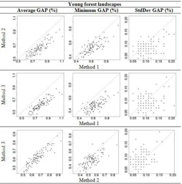
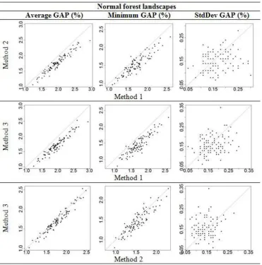
Pairwise comparisons between the methods for the aver-age and minimum GAP, and for the averaver-age first feasible iteration for young, normal and old forest landscapes are shown in Figures 1, 2, 3 and 4, respectively. When dots (datasets) are far from the reference line, this means that the difference in performance between the methods for that specific dataset is big.
Table 2: p-values from pairwise Wilcoxon signed-rank statistical tests for each criterion (columns). Within a forest landscape each criterion and method is represented by one hundred values (number of datasets). *** is significance level =0.01, ** is significance level =0.05, * is significance level =0.10
Forest landscape
Methods compared
Average GAP
Minimum GAP
StdDev GAP
Average first feasible iteration Young 1 vs 2 1.91E-18 *** 1.09E-16 *** 1.47E-08 *** 1.98E-18 ***
1 vs 3 1.93E-18 *** 4.32E-18 *** 2.41E-03 *** 1.98E-18 *** 2 vs 3 1.08E-12 *** 1.79E-12 *** 2.65E-03 *** 1.98E-18 *** Normal 1 vs 2 1.96E-18 *** 8.27E-17 *** 0.001225 *** 1.98E-18 *** 1 vs 3 1.96E-18 *** 2.22E-18 *** 0.019453 ** 1.98E-18 *** 2 vs 3 6.15E-11 *** 6.94E-08 *** 0.182724 1.98E-18 *** Old 1 vs 2 7.76E-17 *** 4.47E-16 *** 0.038134 ** 1.06E-17 *** 1 vs 3 3.44E-18 *** 9.89E-16 *** 0.979267 1.98E-18 *** 2 vs 3 0.701870 0.194507 0.054423 * 1.98E-18 ***
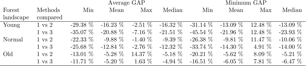
Table 3: Relative difference between Method 1 against Method 2 and 3 for the criteria Average and Minimum GAP.
Average GAP Minimum GAP
Forest landscape
Methods compared
Min Mean Max Median Min Mean Max Median
Young 1 vs 2 -29.38 % -16.23 % -2.51 % -16.32 % -31.14 % -13.09 % 12.48 % -13.09 % 1 vs 3 -35.07 % -20.88 % -7.16 % -21.51 % -45.54 % -21.96 % 12.48 % -23.93 % Normal 1 vs 2 -22.33 % -9.88 % -1.40 % -9.39 % -26.38 % -9.81 % 11.47 % -10.06 % 1 vs 3 -25.68 % -12.84 % -2.76 % -12.32 % -33.74 % -14.30 % 4.91 % -14.00 % Old 1 vs 2 -13.01 % -5.28 % 14.37 % -5.18 % -20.21 % -5.62 % 8.09 % -5.21 % 1 vs 3 -11.71 % -5.20 % 1.63 % -4.94 % -16.51 % -6.05 % 7.81 % -6.47 %
young and normal forest landscapes when comparing Method 1 against Methods 2 and 3. However, when comparing Method 2 and 3, no special trends regard-ing the average and minimum GAP were observed. The statistical test performed (Table 2) confirmed these ob-servations. Moreover, in all datasets the minimum GAP never reached the value zero, i.e. an optimal solution was never found.
The standard deviation of the GAPs obtained for a dataset may be used as a measure to describe the con-sistency of the results obtained by each method. Having as reference the values in the axis (Figures 1, 2 and 3), all the methods become less consistent as the forests get older, i.e. standard deviations of the GAPs obtained in young forest landscapes are smaller than in normal for-est landscapes which again are smaller than in old forfor-est landscapes. In general, the standard deviations of the GAPs obtained by Method 2 were slightly smaller than for the other two methods, but exceptions occur in old forest landscapes, since for some datasets the standard deviation of GAP observed was considerably higher com-pared to the other two methods (Figure 3). The stan-dard deviations are also in general lower for Method 3 than for Method 1 in all forests landscapes. The
statis-tical test performed (Table 2) confirmed these observa-tions.
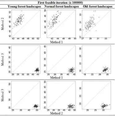
Regarding the average first feasible iteration, Method 2 tends to use more iterations than Methods 1 and 3, while for Method 3 the average iteration when the first feasible solution is found is considerable smaller than for the other two methods. This occurs in all forest landscapes (Figure 4). In addition, having as reference the values in the axis (Figure 4), we observed that the average first feasible iteration tends to appear earlier in old forest landscapes than in young and normal for-est landscapes. The statistical tfor-est performed (Table 2) confirmed these observations.
Figure 1: Scatter plots for young forest landscapes comparing Methods 1 and 2 (upper panels), Methods 1 and 3 (middle panels) and Methods 2 and 3 (lower panels) for average, minimum and standard deviation of GAPs. Dashed lines are reference lines denoting the equality of the methods. Dots (datasets) above the reference line means that the method in Y axis has bigger values than the method in X axis.
GAP obtained by Method 2 was slightly better than the improvement obtained by Method 3, respectively 5.28% and 5.20%. However, for the minimum GAP the im-provement obtained by Method 3 was again higher than the mean improvement obtained by Method 2. More-over, all the medians show that in a considerable number of datasets improvements were obtained.
In all the methods, the number of SA runs finding feasible solutions was high. Only in five and six datasets of old forest landscapes, one run was not capable to find a feasible solution in Methods 1 and 2, respectively.
4
Discussion
Long term forest management planning and optimiza-tion of forest management are complex tasks, and are
Figure 2: Scatter plots for normal forest landscapes comparing Methods 1 and 2 (upper panels), Methods 1 and 3 (middle panels) and Methods 2 and 3 (lower panels) for average, minimum and standard deviation of GAPs. Dashed lines are reference lines denoting the equality of the methods. Dots (datasets) above the reference line means that the method in Y axis has bigger values than the method in X axis.
The methods were tested through a comprehensive experimental design where we, from NFI sample plots comprising a multitude of forest conditions, constructed 300 hypothetical datasets characterized by three differ-ent initial age class distributions (young, normal and old). Our experimental design with a large number of datasets provides a more solid base for evaluation of the developed methods as compared to many previous works with relatively few datasets (e.g. O’Hara et al., 1989; Boston and Bettinger, 1999; Falc˜ao and Borges, 2001, 2002; Crowe and Nelson, 2003). A large num-ber of datasets is important because of the stochastic nature of the method applied (SA). Consequently, this enables better assessments of the impacts of using differ-ent ways to introduce bias in the selection of MUs. The grid configuration of the forest landscapes with equal cell
(stand) size (1 ha) was also important to exclude factors that may influence the evaluation of the methods, for instance the number of neighbors (Li et al., 2010) and the area of each MU. Even controlling such conditions in the experimental design it could be interesting to as-sess the performance of the methods in different forest conditions such as MUs with different size and shape.
Figure 3: Scatter plots for old forest landscapes comparing Methods 1 and 2 (upper panels), Methods 1 and 3 (middle panels) and Methods 2 and 3 (lower panels) for average, minimum and standard deviation of GAPs. Dashed lines are reference lines denoting the equality of the methods. Dots (datasets) above the reference line means that the method in Y axis has bigger values than the method in X axis.
for old forest landscapes none of the methods (Method 2 and 3) outperformed the other in regards to the objec-tive function values. These results agree with our expec-tations; first because the results of Borges et al. (2014) in general showed that introducing bias through static search vectors in the MU selection performed better than the conventional method, and second because by select-ing some MUs accordselect-ing to relevant criteria (manage-ment problem dependent) and by changing these selec-tion probabilities dynamically, achieving better soluselec-tions is more likely.
When comparing the standard deviations of the GAPs, in general within a forest landscape, the solu-tions obtained from each method were similar (Table 2). Furthermore, as found in McDill and Braze (2000) old forest problems are more difficult to solve, and the
Figure 4: Scatter plots for the average first feasible iteration in all forest landscapes comparing Methods 1 and 2 (upper panels), Methods 1 and 3 (middle panels) and Methods 2 and 3 (lower panels). Dashed lines are reference lines denoting the equality of the methods. Dots (datasets) above the reference line means that the method in Y axis has bigger values than the method in X axis.
function is more appropriate than the penalty function applied in the work of Borges et al. (2014).
Regarding the average first iteration when a feasible solution is found, there was undoubtedly a difference between the methods. Method 2 needs more iterations than Method 1 to find the first feasible solution while Method 3 uses considerably less iterations, showing that the bias introduced in MU selection in order to mitigate the two types of constraints was successful (Figures 3, 2 and 3). The value of that solution might not be very good. However, it can be used as a starting point for any other technique or the subset of following feasible solu-tions found can be used as initial population in evolution programs. When comparing Methods 1 and 2 these re-sults are not entirely in agreement with Borges et al. (2014), where only in old forest landscapes it was
evi-dent that Method 2 in average needed more iterations to find the first feasible solution. This difference in results is due to the new penalty function applied.
to assess the impacts of using different weighting alter-natives.
Heinonen and Pukkala (2004) showed that performing changes in two MUs are better than in only one MU and that this may improve the quality of the solution. Thus, an interesting challenge for future research could be not only applying dynamic search vectors but also to extend dynamically the size of the solution neighborhood. This could for instance be useful when solving adjacency vio-lations, since they can occur in different disjoint cliques of MUs. Another interesting extension for the dynamic approach could be the introduction of bias also in the selection of the treatment schedules after the MUs are selected (e.g. Baskent and Jordan, 2002).
Spatial considerations and adjacency constraints are important aspects of long term forest planning. It is therefore crucial to develop efficient tools for decision support in forestry that are able to handle these aspects. SA is one of the most used metaheuristics to address this type of forest planning problems. Our work demon-strates that not only the parameterization of SA is im-portant for the quality of the solutions but also the way the search in the solution space is performed. Moreover, guiding the search dynamically towards more promis-ing areas of the solution space includpromis-ing mechanisms to mitigate constraints violations (Method 3) seems to be a better strategy than using static methods (Methods 1 and 2), and will in general produce higher objective function values, i.e. lower average and minimum GAPs.
5
Conclusions
Introducing bias in the candidate solution generator selecting MUs in SA (Methods 2 and 3) improved the performance compared to the conventional method (Method 1) when forestry planning problems with ad-jacency and sequential flow constraints were addressed. Considerable improvement and consistency in the ob-jective function value of the solutions was also achieved by means of a new penalty function and by introduc-ing the bias for selectintroduc-ing MUs dynamically (Method 3). The mean improvement for the average GAP ob-tained by Method 3 for young, normal and old forest landscapes was 20.88%, 12.84% and 5.20%, respectively. Whereas for the minimum GAP the mean improvement was 21.96%, 14.30% and 6.05% for young, normal and old forest landscapes, respectively. Introducing a dy-namic bias in MUs selection considering the mitigation of constraints also shortened the appearance of the first feasible solution compared to the static methods. More-over, not only the parameterization of the SA but also the way the search of the solution space is performed is important for the quality of the solutions.
Acknowledgements
This work was funded through the Norwegian Bioenergy Innovation Centre (CenBio) by the Research Council of Norway, a number of industrial partners and participat-ing research institutions, among them the Norwegian University of Life Sciences. The authors would like to thank Isabel Martins, for help on the mathematical for-mulation of the problem presented in the manuscript. The authors would like also to thank the anonymous re-viewers for their comments that improved the content of this paper.
References
Barrett, T. M., Gilless, J. K., 2000. Even-aged restric-tions with sub-graph adjacency. Annals of Operarestric-tions Research 95(1), 159175.
Baskent, E. Z., Jordan, G. A., 2002. Forest land-scape management modeling using simulated anneal-ing. Forest Ecology and Management 165(1-3), 29-45.
Baskent, E. Z., Keles, S., 2005. Spatial forest planning: A review. Ecological Modelling 188(2-4), 145-173.
Bettinger, P., Graetz, D., Boston, K., Sessions, J., Chung, W., 2002. Eight heuristic planning techniques applied to three increasingly difficult wildlife planning problems. Silva Fennica 36(2), 561584.
Bettinger, P., Kim, Y., 2008. Spatial Optimisation-Computational Methods. In Designing Green Land-scapes, Gadow, K., T. Pukkala (eds.). Springer, New York. pp. 111-135
Bettinger, P., Sessions, J., Boston, K., 2009. A review of the status and use of validation procedures for heuristics used in forest planning. Mathematical and Computational Forestry & Natural-Resource Sciences (MCFNS) 1(1) 2637.
Borges, P., Eid, T., Bergseng, E., 2014. Applying simu-lated annealing using different methods for the neigh-borhood search. European Journal of Operational Re-search 233(3), 700-710.
Boston, K., Bettinger, P., 1999. An analysis of Monte Carlo integer programming, simulated annealing, and tabu search heuristics for solving spatial harvest scheduling problems. Forest Science 45(2), 292301.
Brumelle, S., Granot, D., Halme, M.,Vertinsky I., 1998. A tabu search algorithm for finding good forest har-vest schedules satisfying green-up constraints. Euro-pean Journal of Operational Research 106(2-3), 408-424.
Chibante, R., 2010. Simulated Annealing Theory with Applications. Sciyo. Rijeka ,Croatia.
Crowe, K., Nelson, J. D., 2003. An Indirect Search Algo-rithm for Harvest-Scheduling Under Adjacency Con-straints. Forest Science 49(1), 1-11.
Dowsland, K.A., 1995. Simulated Annealing. In Mod-ern Heuristic Techniques for Combinatorial Problems. (ed. Reeves, C.R.), McGraw-Hill
Falc˜ao, A. O., Borges. J. G., 2001. Designing an evo-lution program for solving integer forest management scheduling models: an application in Portugal. Forest Science 47(2), 158168.
Falc˜ao, A. O., Borges, J. G., 2002. Combining random and systematic search heuristic procedures for solv-ing spatially constrained forest management schedul-ing models. Forest Science 48(3) 608621.
Gobakken, T., 2003. Brukerveiledning til SGIS- et skog-lig geografisk informasjonssystem. Versjon 2.1. 26 p. Unpublished user manual. ( In Norwegian.)
Goycoolea, M., Murray, A. T., Vielma, J. P., Weintraub, A., 2009. Evaluating Approaches for Solving the Area Restriction Model in Harvest Scheduling. Forest Sci-ence 55(2), 149-165.
Heinonen, T., Pukkala, T. 2004. A comparison of one-and two-compartment neighbourhoods in heuristic search with spatial forest management goals. Silva Fennica 38(3) 319332.
Hoen, H. F. Eid, T. 1990. A model for analysis of treat-ment strategies for a forest applying standvice simula-tions and linear programming. Rapp. Nor. Inst. Skog-forsk. 9/90, 1-35. (In Norwegian with English sum-mary.)
Kirkpatrick, S., Gelatt, C. D.,Vecchi. M. P., 1983. Op-timization by simulated annealing. Science 220(4598), 671-680.
Li, R., Bettinger, P., Boston, K., 2010. Informed Devel-opment of Meta Heuristics for Spatial Forest Planning Problems. The Open Operational Research Journal 4, 1-11.
Liu, G., Han, S., Zhao, X., Nelson, J., Wang, H., Wang, W., 2006. Optimisation algorithms for spatially con-strained forest planning. Ecological Modelling 194(4), 421-428.
Lockwood, C., Moore, T., 1993. Harvest scheduling with spatial constraints: a simulated annealing approach. Canadian Journal of Forest Research 23(3), 468478.
McDill, M.E., Braze, J., 2000. Comparing adjacency constraint formulations for randomly generated forest planning problems with four age-class distributions. Forest Science 46(3), 423-436.
McDill, M. E., Rebain, S., Braze, J., 2002. Har-vest scheduling with area-based adjacency constraints. Forest Science 48(4), 631-642.
Murray, A. T., Church, R. L., 1995. Heuristic solution approaches to operational forest planning problems. OR Spektrum 17(2-3) 193-203.
Murray, A. T., Church, R. L., 1996a. Constructing and selecting adjacency constraints. INFOR, 34: 232–248.
Murray, A. T., Church, R. L., 1996b. Analyzing cliques for imposing adjacency restrictions in forest models. Forest Science 42(2) 166175
Murray, A. T., 1999. Spatial Restrictions in Harvest Scheduling. Forest Science 45(1), 45-52.
O’Hara, A., Faaland, B., Bare, B. B., 1989. Spa-tially constrained timber harvest scheduling. Cana-dian Journal of Forest Research 19(6), 715-724.
Rebain, S., McDill, M. E., 2003. A mixed-integer for-mulation of the minimum patch size problem. Forest Science, 49(4), 608–618.
Shan, Y., Bettinger, P., Cieszewski, C. J., Li, R.T., 2009. Trends in spatial forest planning. Mathematical and Computational Forestry & Natural-Resource Sciences (MCFNS) 1(2), 86-112
Strimbu, B. M., Innes, J. L., Strimbu, V. F., 2010. A deterministic harvest scheduler using perfect bin-packing theorem. European Journal of Forest Re-search 129(5), 961974.
Vielma, J. P., Murray, A. T., Ryan, D. M., Weintraub, A., 2007. Improving computational capabilities for ad-dressing volume constraints in forest harvest schedul-ing problems. European Journal of Operational Re-search, 176(2), 12461264.
Weintraub, A., Murray, A. T., 2006. Review of combi-natorial problems induced by spatial forest harvesting planning. Discrete Applied Mathematics 154(5), 867-879.
¨
Ohman, K., Eriksson, L. O., 1998. The core area con-cept in forming contiguous areas for long-term for-est planning. Canadian Journal of Forfor-est Research 28, 10321039.
¨
Ohman, K., 2000. Creating continuous areas of old for-est in long-term forfor-est planning. Canadian Journal of Forest Research, 30, 1817-1823.
¨
Ohman, K., Eriksson, L. O., 2002. Allowing for spatial consideration in long-term forest planning by linking linear programming with simulated annealing. Forest Ecology and Management 161(1-3), 221-230.
¨