Model-Free Uncalibrated Visual Servoing Using Recursive Least Squares

Model-Free Uncalibrated Visual Servoing Using

Recursive Least Squares

Miao Hao, Peter Deuflhard, Zengqi Sun, Masakazu Fujii

Department of Computer Science and Technology, Tsinghua University, Beijing, China. Zuse Institute Berlin (ZIB), Berlin, Germany.

Corporate Research and Development, IHI Co.,Ltd., Yokohama, Japan.

Email: [email protected]; [email protected]; [email protected]; masakazu [email protected].

Abstract— In this paper, a model free uncalibrated visual servoing algorithm based on recursive least squares is proposed and discussed in depth. No robot kinetics or dynamics, camera calibration or target model to be tracked would be ever needed. Based on the brief retrospection of RLS filter as well as its theoretical analysis, i.e. Wiener-Hopf condition, the core uncalibrated visual servoing algorithm based on recursive least squares is explored in detail. The experimental results of both static and moving targets applied on a Puma-560 6DOFs industrial robot simulation verifies its performances.

Index Terms— Visual Servoing, Jacobian Estimate, Nonlin-ear Control, Adaptive RLS

I. INTRODUCTION

For numerous industrial applications of robotics and automation today, robot control with visual clues, or more technically, visual servoing, has demonstrated impressive power in large volumes of industries applications and has been regarded as one of the most promising research realms in Artificial Intelligence and Robotics [1]. Techni-cally, the current visual servoing methods could be catego-rized into two main types, Position Based Visual Servoing (PBVS) and Image Based Visual Servoing (IBVS) respec-tively (Kragic, 2001). According to [2][3][1], most of the visual servoing systems reported in previous literature, have to utilize the robot and especially the camera model, i.e. camera calibration is needed, if satisfying results and performance required [3]. It’s well known that the typical camera calibration process is in most cases elaborate, time-consuming yet not robust enough to system and environmental noises. In other word, a high accuracy camera calibration is obtained usually in constructed or at least semi constructed environment.

Therefore, the uncalibrated visual servoing without the priori knowledge of robot kinetics, dynamic as well as camera calibration was paid extensive attentions in recent years [4][5]. [6] presented uncalibrated visual servoing for static targets using fixed cameras. [7] improved the

This paper is based on “Uncalibrated Visual Servoing Using Recur-sive Least Squares,” by M. Hao, Z.Q. Sun, M. Fujii, W. Song, which appeared in the Proceedings of the 2007 IEEE International Conference on Systems, Man and Cybernetics (SMC), Montreal, Canada, October 2007. c°2007 IEEE.

This work is supported by the international collaboration project with IHI, Japan, and also in part by the 973 High Tech. Programs of China (2002CB312205).

control scheme to eye-in-hand stereo tracking of moving targets using static reference points to estimate the target motion, through the online estimation of Jacobian matrix. [8] introduced a Broyden method in non-linear least square optimization using a trust region and [9] as a review, expanded them with convergence analysis and proof. Especially, [10] proposed in detail, a dynamic visual servoing method to tracking a moving target, i.e. the velocity estimate was also done within the estimation of Jacobian matrix and compared the partitioned Broyden method with the Recursive Gauss-Newton method in depth with a 6DOF robot simulation, [9] has investigated an improved control law for moving target yet unfortu-nately, its convergence analysis seems incomplete which we would discussed later.

Theoretically, the best result reported in previous lit-erature is [10] which is based on the non-linear opti-mization of affine invariance and adaptive algorithms, which has been utilized from [6][11] to [9][10] without much change. However, the Broyden method could be categorized as local Newton method and has to face the local minima and even stability and robustness issues. The global Newton methods have shown the preponderance versus the local Newton methods, and they are drawing more attentions in recent year [12].

This paper contributes in following three points: (1) an uncalibrated eye-in-hand visual servoing using adap-tive recursive squares (VS-ARLS) versus VS-RLS is proposed, analyzed in detail and verified by a 6DOFs Puma560 simulation; (2) the evaluation criterions of the visual servoing algorithm in time-varying system are introduced; (3) the asymptotic stability analysis of the proposed algorithm in an affine contravariance perspec-tive.

Figure 1. The structure of an RLS filter. This figure is refered to [13].

Besides, experimental results would be discussed in Sec-tion V and performance analysis in SecSec-tion VI. Finally, Section VII would be the conclusive section summarizing and indicating the research topics in the future.

II. CLASSICALUNCALIBRATEDVISUALSERVOING USINGRECURSIVELEASTSQUARES

In this section, the classical uncalibrated visual ser-voing using recursive least squares is introduced and discussed briefly, for the incoming comparison of the new algorithm using adaptive recursive least squares.

A. Recursive Least Squares

It’s constructive to have a retrospection of Recursive Least Squares (RLS) from which the classical VS-RLS would be deduced. A structural view of RLS filter is shown in Fig. 1.

Since the observable data is variable, the cost function to be minimized could be expressed asE(n)wherenis the variable length of the observation data. And the cost function is often expressed in a weighting factor way, i.e.

E(n) =

n

X

i=1

β(n, i)|e(i)|2 (1)

where β(i) is the filter coefficient and e(i) the error between desired response d(i) and current output y(i), i.e.

e(i) = d(i)−y(i)

= d(i)−wH_(n)u(n) (2) and

u(i)=[u(i), u(i−1), ..., u(i−M+ 1)]T

w(n)=[w0(n), w1(n), ..., wM−1(n)]T (3)

where u(i) is the input signal vector and w(n) the weighting vector.

Let

β(n, i) =λn−i, i= 1,2, ..., n (4)

where λ is noted as forgetting factor to forget the past information. The optimal solution of (1) is then equal to the following Wiener-Hopf equation

Φ(n)w(n) =˜ z(n) (5)

where

Φ(n)=Pn

i=1

λn−i_u(i)uH_(i)

z(n)=Pn

i=1

λn−i_u(i)d∗_(i) (6)

which could be re-written in recursive form and expanded using matrix inversion lemma, then we immediately have the exponentially weighted recursive least squares algo-rithm [13]

Initialization:

e

w(0) =0;P=δ−1_{Iis a small positive constant.}

Iteration body: for n=1,2,...,N

k(n)= λ

−1_P(n−1)u(n) 1 +λ−1_uH_{(n)P(n−1)u(n)}

ξ(n)=d(n)−wH_(n−1)u(n)

w(n)=w(n−1) +k(n)ξ(n)

P(n)=λ−1_{P(n−1)−λ}−1_k(n)uH_(n)P(n−1) (7)

B. Uncalibrated Eye-in-hand Visual Servoing Using Re-cursive Least Squares

The task description of the uncalibrated eye-in-hand visual servoing could be described as follows [12]: given a robotRand an eye-in-hand cameraCwithout calibration, the objective is to move the robot from the eye-in-hand image feature y(θ) under current joint value θ, to the desired image feature y∗_{(θ). No robot kinetics or}

dynamics model needed. Nor does the camera model. The error function is defined as

f(θ,t) =y(θ)−y∗_{(t) (8)}

The squared error function is defined as

F(θ, t) =1 2f

T_{(θ, t)f(θ, t) (9)}

And the squared error function could be expressed in first order Taylor form as

F(θ+ ∆θ, t+ ∆t) =F(θ, t) +∂F

∂θ∆θ+∂∂tF∆t+O(∆θ,∆t) (10) considering that the sampling period is assumed to be a constant, the minimum of F(θ,t)could be calculated as

∂F(θ+ ∆θ, t+ ∆t)

∂θ = 0 (11)

Omit the high order infinite population O(∆θ,∆t), approximately we have

∂F ∂θ +

∂2_F ∂θ2∆θ+

∂2_F

∂θ∂t∆t= 0 (12)

then

∆θ=−

µ ∂2_F ∂θ2

¶−1µ ∂F

∂θ + ∂2_F ∂θ∂t∆t

¶

Substituting (13) with (9) and (10) would result in

∆θ=−¡JTJ+S¢−1JT µ

f+∂f ∂t∆t

¶

(14)

where

J= ∂f

∂θ,S=∂J

T

∂θ f,∂∂θF =JTf, ∂2_F

∂θ∂t=JT ∂∂tf,∂

2_F

∂θ2 =JTJ+S,

(15)

Note the definition J=∂f/∂θ is known as composite Jacobian matrix. Moreover, since Sis system dependent and actually difficult to estimate, yet it could be regarded as an infinite population, because when the robot position is near the desired, the error function f(θ,t) could be regarded as zero. Therefore, we could re-write (15) as

∆θ=−

³ ˜ JTk˜Jk

´−1 ˜ JTk

µ f +∂f

∂t∆t ¶

(16)

where ˜J stands for the estimation of the composite Jacobian matrix at theKth iteration. And (16) is the joint value update formula.

Besides, the affine model of error function is defined as

mk(θ, t) =f(θk, tk) +J˜k(θ−θk) +∂fk

∂t(t−tK) (17)

which could be regarded as also the first order expan-sion ofmk(θ, t) at(θk, tk) and the corresponding target function is

minE(k)=kP−1

i=0

λk−i−1_k∆m

kik2

∆mki=mk(θi, ti)−mi(θi, ti)

=£fk−fi−∂_∂tfk(tk−ti)

¤

−Jkhki

=[fk−fi]−Jkhki

(18)

where we denote

hki=(θk−θi)

hk=tk+1−tk (19)

Now it’s time to look backward at the RLS algorithm. Compare (18) to (7) with (1) and (4) in mind, if we make the following substitutions

d→∆f =fk−fk−1 wH_→J

k =

£ ˜

Jk (˜ft)k−1 ¤

u→h= ·

θk−θk−1 tk−tk−1

¸ (20)

where scalar expanded to a vector, and column vector to rectangle matrix, then the complete description of the VS-RLS algorithm could be expressed as [10][12]

Initialization:

Given f :R

n _→Rm_{;θ0, θ1∈R}m×n_;

(fet)0∈Rm×1;P0∈Rn+1×n+1;λ∈(0,1]; Iteration body:

∆f=fk−fk−1;hθ=θk−θk−1;ht=tk−tk−1

h= ·

θk−θk−1 tk−tk−1

¸

Jk=

£ ˜

Jk (˜ft)k−1 ¤

∆Jk=(∆f−Jk−1h) ¡

λ+hT_P k−1h

¢−1 hT_P

k−1 Jk=Jk−1+ ∆Jk

Pk=λ1

h

Pk−1−Pk−1hh T_P

k−1

λ+hT_P k−1h

i

θk+1=θk−

³ ˜ JT

k˜Jk

´−1³ ˜ JT

kfk+˜JTk(˜ft)kh

´

(21)

III. PERFORMANCEEVALUATION OFTIME-VARYING SYSTEMTRACKING

For stationary environment where both the statistical variables and the error performance surface are fixed, the transient or natural gradient based method in most cases would result in an optimum or at least near optimum performance. Yet when it comes to a time-vary system where the statistical description of the system becomes non-stationary or dynamic, the error performance surface is no longer fixed and therefore a new evaluation of tracking performance is added.

As [13] stated, tracking is a steady-state phenomenon, yet the statistical variations of the environment has to be slow enough for tracking to be feasible. Then the concept of degree of nonstationarity is introduced as [14]

α= 

E h¯

¯_wH_(n)u(n)¯_¯2i

E h

|v(n)|2

i 

 1/2

(22)

where w(n) and v(n) are process noise vector and measurement noise respectively.

Technically, the criterions for tracking evaluation could be categorized as follows: mean-square deviation and displacement respectively.

A. Mean Square Deviation

One of the most commonly used merit for tracking evaluation is Mean Square Deviation (MSD), defined as

D(n) =E[|w(n)ˆ −w0(n)|2] (23)

where

D(n)=D1(n) +D2(n) D1(n)=E

h

|w(n)˜ −E[w(n)]˜ |2

i

D2(n)=E

h

|E[w(n)]˜ −w0(n)|2

i (24)

B. Replacement

Another widely used criterion is misplacement define as

M=Jex(n) σ2

v

(25)

whereJex(n)is the excess mean squared error of adaptive filter measured with respect to the varianceσ2

v. Again, the displacement could also be divided into two components as

M(n) =M1(n) +M2(n) (26)

where M1(n) is called noise misadjustment and the second lag misadjustment, in that the estimation noise and lag noise are decoupled in power.

IV. CLASSICALUNCALIBRATEDVISUALSERVOING USINGADAPTIVERECURSIVELEASTSQUARES Taking the discussions and performance evaluation criterions discussed in Section III in mind, one aspect of promoting the performance of system tracking in a RLS form, which is the very case stated in this paper, is to focus on the adaptive tuning of the learning rate λ, i.e. to select the optimal learning rate in every step.

Again, the cost function could be re-defined as

J0_{(n) =} 1

2E[|ξ(n)|

2_{] (27)}

whereξ(n)is the priori knowledge error, i.e.

ξ(n) =d(n)−wH_{(n−1)u(n) (28)}

The partialJ0_{(n), partialλis}

∇λ(n)=∂J_∂λ0(n) =1

2E h

∂ξ(n)

∂λ ξ∗(n) + ∂ξ∗_(n)

∂λ ξ(n)

i

=−1 2E

£

ΨH_{(n−1)u(n)ξ}∗_{(n) +u}H_{(n)Ψ(n−1)ξ(n)}¤ (29) where

Ψ(n) = ∂w(n)

∂λ (30)

Note that in (7) we have

k(n)=P(n)u(n)

w(n)=w(n−1) +P(n)u(n)ξ∗_(n) (31)

and if we denote

S(n) =∂P(n)

∂λ (32)

then it’s easy to have

Ψ(n)=[I−k(n)uH_{(n)]Ψ(n−1) +S(n)u(n)ξ}∗_(n) P(n)=λ−1_P(n−1)−λ−2_{P(n−1)u(n)u}H_(n)P(n−1)

1+λ−1_uH_{(n)P(n−1)u(n)} (33) Differentiating the second equation in (29) yields

S(n) =λ−1_[I−k(n)uH_{(n)]S(n−1)[I−u(n)k}H_(n)]

+λ−1_k(n)kH_(n)−λ−1_P(n)

(34)

Now we are ready to deduce the adaptive learning rate

λ. If we substitute the scalar gradient∇λ(n)with instan-taneous gradient estimation−Re[ΨH_{(n−1)u(n)ξ}∗_(n)],

the adaptively tuned learning rate λis calculated as

λ(n)=λ(n−1)−α∇ˆλ(n)

=λ(n−1) +αRe[ΨH_{(n−1)u(n)ξ}∗_(n)] (35)

where α is a small positive parameter. Now we’ve suc-cessfully expand the standard RLS algorithm into adaptive recursive least squares (ARLS) where actually fixed λ

is expanded to time-varying λ(n). The ARLS could be described as follows

Initialization:

e

w(0) =0;P=δ−1_{Iis a small positive constant.}

Iteration body: for n=1,2,...,N

k(n) = _1+λ−λ1−_u1HP₍(_nn₎−_P1)_(nu₋(n₁₎)_u(n) ξ(n) =d(n)−wH_(n−1)u(n)

w(n) =w(n−1) +k(n)ξ(n)

P(n) =λ−1_{P(n−1)−λ}−1_k(n)uH_(n)P(n−1)

λ(n) = [λ(n−1) +αRe[ΨH_{(n−1)u(n)ξ}∗_(n)]]λ+

λ− S(n) =λ−1_{(n)[I−k(n)u}H_{(n)]S(n−1)[I−}

u(n)kH_{(n)] +λ}−1_(n)k(n)kH_(n)−λ−1_P(n) Ψ(n) = [I−k(n)uH_{(n)]Ψ(n−1) +S(n)u(n)ξ}∗_(n)

(36)

where λ+ and λ−1 stand for upper and lower bound

truncation respectively and its equation typical Newton Leibniz formula. Empirically, λ+ is preferred to near 1

yet λ−1plays a critical role in the tracking performance.

Similarly, we would have immediately the uncalibrated eye-in-hand visual servoing using adaptive recursive least squares (VS-RLS) as

Initialization:

Given f :R

n _→Rm_{;θ0, θ1∈R}m×n_;

(fet)0∈Rm×1;P0∈Rn+1×n+1;λ∈(0,1]; Iteration body:

∆fk =fk−fk−1;hθ=θk−θk−1;ht=tk−tk−1 h =

·

θk−θk−1 tk−tk−1

¸

Jk =

£ ˜

Jk = (˜ft)k−1 ¤

∆Jk = (∆fk−Jk−1h) ¡

λn+hTPk−1h ¢−1

hT_P k−1 Jk =Jk−1+ ∆Jk

Pk = _λ1_n

h

Pk−1−Pk−1hh T_P

k−1

λ+hT_P k−1h

i

θk+1 =θk−

³ ˜ JT

k˜Jk

´−1³ ˜ JT

kfk+˜JTk(˜ft)kh

´

λn = [λn−1+α(∆fk−Jk−1h)0Ψnh]λ_λ+₋

Sn =λ−n1[I−knh0]Sn−1[I−hkHn]

+λ−1

n knkHn −λ−n1Pn

Ψn = [I−knuHn]Ψn−1+ (∆fk−Jk−1h)(Snh)0 (37)

V. EXPERIMENTALSIMULATIONS

-1 -0.5

0 0.5

1

-1 -0.5 0 0.5 1 -1 -0.5 0 0.5 1

X Y

Z

Puma 560 IBVS Simulation Using Puma 560

x y z

Figure 2. The simulation of 6DOF Puma560 using Robotics Toolbox for MatLab (Corke, 1996) as well as the target in world coordination system.

-200 -150 -100 -50 0 50 100 150 -200

-150 -100 -50 0 50

Eye-in-hand Vision Simulation Using Puma 560

Figure 3. The eye-in-hand vision of Puma560 where the red region indicates the desired image feature and the blue the current.

discussed. The eye-in-hand camera is assumed to be coincident with the final joint, i.e. the end grasper pose and position is those of the camera. The robot simulation toolbox is shown in Fig. 2, including the initial robot pose and position as well as the target.

The sampling period is 50ms and the system runs at 20Hz. The target is selected as an irregular quadrangle whose homogeneous world coordination vector is

PW(A, B, C, D) =

   

0.700 0.700 0.700 0.700

−0.100 0.300 0.100 −0.200 0.200 0.700 0.800 0.600 1.000 1.000 1.000 1.000

   

(38) Note that the selection of this quadrangle is to avoid the potential singularity of Jacobian matrix. Experimental results in [9][10] are of square targets yet the desired feature vector in eye-in-hand image plane is not, for the same reason.

The focus length isf = 0.004mand the pixel projec-tion ratio isP = 30,000pixel/m. The static and moving target tracking are done respectively. The additive uniform noise to the coordination of the image plane is 0.2 pixel. Let the Z axis and Y axis in the end grasper coordi-nation system be coincidental with the X and Y axis in the eye-in-hand image plane, the coordination translation

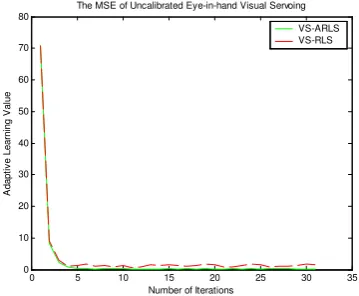
0 5 10 15 20 25 30 35 0

10 20 30 40 50 60 70 80

The MSE of Uncalibrated Eye-in-hand Visual Servoing

Number of Iterations

A

d

a

p

ti

v

e

L

e

a

rn

in

g

V

a

lu

e

VS-ARLS VS-RLS

Figure 4. The MSE curves of static target tracking using VS-RLS and VS-ARLS. The solid line is VS-ARLS and the dotted VS-RLS. The average of MSE using VS-ARLS is 1.863.

from P(x, y, z), the end grasper coordination system to the image plane system (Ix, Iy)is

· Ix

Iy

¸

= f·P x

· y z

¸

(39)

A. Initial Jacobian Matrix Estimation

The initial Jacobian matrix estimation is believed to impact dramatically the performance of the algorithm, i.e. if improperly chosen, the servoing process does not even work and the robot seems out of control.

In [16], the tiny displacements of each joint and the corresponding displacements of the feature vector consist of n pairs

[(dθ0,df0),(dθ1,df1), ...,(dθn,dfn)] (40) and then we have

ΘD= [dθ0,dθ1, ...,dθn]

FD= [df0,df1, ...,dfn]

(41)

Now the initial Jacobian matrix estimation is calculated as

˜

J0=FD(ΘD)−1 (42)

B. Static Target Tracking

The curves of MSE and joint value of static target tracking are shown in Fig. 4 and Fig. 5 respectively. The convergence speeds of VS-ARLS and VS-RLS are nearly same, yet the average MSE of VS-ARLS is better than that of VS-RLS. The average MSE of VS-ARLS in static target tracking is 1.863pixels.

C. Dynamic Target Tracking

The ellipse motion curve of the target is

½

y=−0.1 + 0.1 sin(1∗ht∗tk)

0 20 40 60 80 100 120 -2

0 2 4 6 8 10 12

Joint Value Curve of Visual Servoing

Number of Iterations

J

o

in

t

V

a

lu

e

i

n

D

e

g

re

e

Figure 5. The joint value curves of static target tracking of VS-ARLS.

0 20 40 60 80 100 120 140 160 0

5 10 15 20 25 30 35 40 45

The MSE of Uncalibrated Eye-in-hand Visual Servoing

Number of Iterations

A

d

a

p

ti

v

e

L

e

a

rn

in

g

V

a

lu

e

VS-ARLS VS-RLS

Figure 6. The MSE curves of moving target tracking using VS-RLS and VS-ARLS. The solid line is VS-ARLS and the dotted VS-RLS. The average of MSE using VS-ARLS is 2.863.

VI. PERFORMANCEANALYSIS ANDDISCUSSION In this section, the performance of the proposed algo-rithm is analyzed critically, in a pros and cons manner. We could summary this problem in multiple perspectives. Theoretically, this algorithm could be categorized into residual based affine invariance/contravariance Newton algorithms in terms of Numerical Analysis, or an online estimation of a highly nonlinear, high dimensional, ill-conditioned and even time-varying (if tracking moving target) kernel matrix, the Jacobian matrix denoted as in terms of System Identification or, a Finite Impulse Response filter to attack an augmented tap vector, which is exactly the Jacobian matrix applied to ”filter” the robot joint value vector as input and output the image feature vector or finally, a Visual Servoing issue to drive the robot arm to a desired pose and position in terms of Robotics, the most initiative point of view.

A. The pros of this algorithm

For a model free uncalibrated visual servoing algo-rithm, its performance demonstrated is satisfying and its pros are easy to have: (1) do not need robot kinetics or dynamics; (2) do not need the all consuming yet delicate process camera calibration; (3) is capable to track any target where current and desired feature vector could be extracted; (4) do not need any pre or pose process such as system modeling or environmental interaction.

0 20 40 60 80 100 120 140 160 -30

-20 -10 0 10 20 30

Joint Value Curve of Visual Servoing

Number of Iterations

J

o

in

t

V

a

lu

e

i

n

D

e

g

re

e

Figure 7. The joint value curves of moving target tracking of VS-ARLS.

B. The cons of this algorithm

Yet we would like to concentrate more on its cons, which might be brought along as all the pro items, turning peach into lemon.

(1) Local minima is inevitable for a inherently local Newton based algorithm. As well known to all, local New-ton algorithm would suffer trapping in a small gradient zone anyway. Technically, this algorithm tries to climb the complicated shaped and full-of-pitfall hill anyway. Whenever the transient gradient estimation is not that accurate, it snares you.

(2) Moreover, as same to most local Newton al-gorithms, it’s initial estimation sensitive, i.e., a ”good enough” initial estimation of the kernel Jacobian ma-trix is crucial for a successful visual servoing process. Attacking (1) and (2) simultaneously would result in a global expansion of the current algorithm, one of the most promising improvements. Note that the construction of global Newton based visual servoing algorithm, which is capable to track the target more flexibly, is strongly rec-ommended in the affine invariance framework introduced for the very reason that the theoretical analysis of affine invariance algorithms would directly lead to construction of algorithms.

(3) Most of its pros could be regarded as autonomous system identification or filtering, yet frankly speaking it’s quite a challenge for a classical RLS filter to estimate such a highly nonlinear and ill-conditioned kernel. In such a situation, it is more vulnerable to system modeling errors and noises. Since it has to utilize every bit of information obtained from each step contaminated by system model-ing and noises, over-fittmodel-ing is some extent possible where the online adjustment of the kernel would reluctantly influenced by noises. To overcome that, tradeoff between having more information to learn and resisting the noise and error contamination has to be made, resulting in empirical adjustment of the forgetting factor . Therefore, a more explicit function linking the error-and-noise and the forgetting factor would be constructive to achieve better performance.

industrial robot applied consist of rotational joints, the Jacobian matrix runs into singular or at least highly ill-conditioned in extreme cases such as the adjacent two rods aligns, let alone all kinds of 6DOFs robots. That’s partial reason of its ill-condition. To solve that inherent problem is substantially challenging, yet a natural choice is to introduce an artificial potential field like method to circumvent this issue, that is, when the robot runs into a highly ill-conditioned pose or position, the weighted potential field would hinder it from moving forward to further singular zone.

ACKNOWLEDGMENT

The corresponding author of this paper sincerely thanks to Prof./Dr. H.Lipkin as well as Dr. J.A.Piepmeier for fruitful and constructive discussion with the topic. Be-sides, he also acknowledges the anonymous reviewer(s) of the Journal of Computers for penetrating comments on this paper.

REFERENCES

[1] Hutchinson S., Hager G D, Corke P I, A Tutorial on Visual Servo Control, Robotics and Automation, IEEE Transaction on, Vol. 12, 651-670, Oct, 1996

[2] Kragic D., Visual Servoing for Manipulation: Robustness and Integration Issues, Ph.D. Dissertation, Royal Institute of Tech-nology, Sweden, 2001

[3] Deng L.F., Comparison of Image-Based and Position-Based Robot Visual Servoing Methods and Improve-ments, Ph.D. Disser-tation, Waterloo University, Canada, 2003

[4] Jang W., Bien Z., Feature-based Visual Servoing of an Eye-in-hand Robot with Improved Tracking Performance, IEEE Interna-tional Conference on Robotics and Automa-tion, Vol. 3, 2254-2260, Sacramento, CA, USA, 1991 [5] Malis E., Chaumette F., Theoretical Improvements in the

Stability Analysis of a New Class of Model-free Vi-sual Servoing Methods. Robotics and Automation, IEEE Transactions on, Vol. 18(2), 176-186, 2002

[6] Hosoda K., Igarashi K., Asada M., Adaptive hybrid con-trol for visual servoing and force servoing in an unknown environment, IEEE Robot. Automat. Mag., Vol. 5(4), 39-43, 1998

[7] Tanaka T., Asada M., Hosoda K., Visual tracking of unknown moving object by adaptive binocular visual servoing, Proc. IEEE Int. Conf. Multisensor Fusion and Integration for Intelligent Systems, Vol. 3, 2076-2081, San Francisco, USA, 1999

[8] Jagerand M., Fuentes O., Nelson R., Experimental Eval-uation of Uncalibrated Visual Servoing for Precision Manipulation. Pro-ceedings of IEEE International Con-ference on Robotics and Automation, Vol. 4, 2874-2880, Albuquerque, NM, USA, 1997

[9] Piepmeier J. A., McMurray G. V., Lipkin H., Uncalibrated Dynamic Visual Servoing, Robotics, IEEE Transactions on, Vol. 20(1), 143-147, Feb, 2004

[10] Piepmeier J.A., Lipkin H., Uncalibrated Eye-in-hand Vi-sual Servoing, The International Journal of Robotics Re-search, Vol. 22, 805-819, 2003

[11] Hosoda K., Asada M., Versatile visual servoing without knowledge of true Jacobian, Proc. IEEE/RSJ/GI Int. Conf. Intelligent Robots and Systems, Vol. 1, 186-193, Munich, Germany, Sept. 1994

[12] Hao M., Sun Z.Q., Fujii M., Song W., Uncalibrated Eye-in-hand Visual Servoing Using Recursive Least Squares,

Proc. IEEE Int. Conf. System, Man and Cybernetics, 64-69, Montreal, Canada, 2007

[13] Haykin S., Adaptive Filter Theory 3rd, Englewood Cliffs, Prentive-Hall, New York, USA, 2004

[14] Macchi O., Adaptive Processing: The LMS Approach with Applications in Transmission, Wiley, New York, USA, 1995

[15] Corke P.I., A Robotics Toolbox for MatLab, IEEE Robotics and Automation Magazine., Vol. 3(1), 24-32, Mar, 1996

[16] Zhou L., Guo Z.M., Application of Exploratory Motion in Visual Servoing Method without Calibration, Journal Harbin Univ. Sci.&Tech., Vol. 7(1), 11-13, Feb, 2002 (in Chinese)

[17] Deuflhard P., Newton Methods for Nonlinear Problems: Affine Invariance and Adaptive Algorithms, Springer-Verlag, Berlin, Germany, 2004

[18] Cretual, A., Chaumette, F., Bouthemy, P., Complex Object Tracking by Visual Servoing Based on 2d Image Motion, 14th In-ternational Conference on Pattern Recognition, Vol. 2, 1251-1254, Brisbane, Qld., Australia, 1991 [19] Flandin G., Chaumette F., Marchand E.,

Eye-in-hand/eye-to-hand cooperation for visual servoing. IEEE Interna-tional Conference on Robotics and Automation, Vol. 3, 2741-2746, San Francisco, USA, 2000

[20] Hao M., Sun Z.Q., Uncalibrated Eye-in-hand Visual Servoing Using Adaptive Recursive Least Squares, 17th World Congress of International Federation of Automatic Control, 1021-1026, Chongqing, China, 2008.

[21] Zhao Q.J., Lian G.Y., Sun Z.Q., Survey of Robot Visual Servoing, Control and Decision, Nov, 2001 (in Chinese)

APPENDIX

Historically, the first classical convergence theorems for Newton series methods are Newton-Kantorovich theorem and Mysovskikh theorem respectively. Newton-Kantorovich theorem introduces Newton-Kantorovich quantity

h0=k∆x0kXβ0γ < 1₂ and a convergence ball roundx0 with radius ρ0 ∼1/β0γ. Similarly, Newton-Mysovskikh

theorem introduces Mysovskikh quantity, slightly differ-ent from the previous one, h0 = k∆x0kXβγ < 2 and a convergence ball round x0 with radius ρ ∼ 1/βγ. However, such a quantity is certainly difficult to com-pute in realistic nonlinear systems, if not hopeless [17]. Therefore, it’s the very introduction of affine invariance framework that helps eliminate the gap between theoret-ical convergence analysis and realistic algorithm design and implementation.

Firstly, the contraction factor, or convergence monitor would be introduced as

Θk= k∆θ k+1_k

k∆θk_k (44)

wheneverΘk ≥1for simplicity, the algorithm monitored is classified as ‘not convergent’.

Since the Broyden based method could be classified as Jacobian rank-1 update, then the Jacobian rank-1 update operator is defined as

Ek(J) =I−JkJ−1 (45)

b≤ Θ−η0

1 +η0+4

3(1−Θ)−1

(46)

if

η=η0+ t

(1−b)(1−Θ)

we could have

η+ (1 +η)t <Θ (47)

The proof of Lemma 1 could be accessed at [17]. Theorem 1. For F ∈C1_{(D), F :D ⊂R}n _→Rm_,D convex, if θ∗ _{indicates the unique solution of robot joint}

value with F0_(θ∗_{) nonsingular. For a specified ω < ∞,} θ∈D, the affine contravariance Lipschitz condition

k(F0_(θ

k)−F0(θ∗))(θ−θk)k ≤

ωkF0_(θ∗_)(θ

k−θ∗)kkF0(θ∗)(θ−θk)k (48)

holds. For specified Θ∈(0,1), ifη0 =kE0k <Θ, and

the initial robot joint value condition

b=ωkF0_(θ∗_)(θ0−θ∗_{)k ≤} Θ−η0

1 +η0+ 4/3(1−Θ)−1

(49) holds, the robot joint value series {θk} would converge toθ∗ _{in terms of error as}

kFk+1k ≤ΘkFkk (50)

or in the terms of image feature vector as

kyk+1−y∗k ≤Θkkyk−y∗k (51)

Proof.The Jacobian rank-1 update ofF is

Fk+1 = Fk+

R₁

q=0F0(θk+q∆θk)∆θkdq = R_q1₌₀(F0_(θk_+q∆θ

k)−F0(θ∗))∆θkdq

+(F0_(θ∗_)−J

k)∆θk

(52) Consider the Lipschitz condition (48), (52) yields

kFk+1k ≤

R₁

q=0k(F0(θk+q∆θk)−F0(θ∗))∆θkkdq +k(F0_(θ∗_)J

k−1−I)Fkk

≤ R_q1₌₀ωkF0_(θ∗_)(θ

k+q∆θk−θ∗)k

·kF0_(θ∗_)∆θ

kkdq+kEkFkk

≤ R_q1₌₀ω(kF0_(θ∗_)(1−q)(θ

k−θ∗)k

+kF0_(θ∗_)q(θ

k+1−θ∗)k)

kF0_(θ∗_)∆θ

kkdq+ηkkFkk

= 1

2(bk+bk+1)kF0(θ∗)∆θkk+ηkkFkk

(53) Defining bk =12(bk+bk+1), then

kFk+1 ≤ bkk(Ek−I)Fkkk+ηkkFkk

≤ (bk(1 +ηk) +ηk)kFkk (54)

Now we only have to prove

bk(1 +ηk) +ηk≤ kΘk (55)

The update formula forgk is

gk+1 = gk−F0(θ∗)Jk−1Fk=F0(θ∗)(θk−θ∗)

−Fk+EkFk

= R_s1₌₀(F0_(θ∗_)−F0_(θ∗_+q(θ

k−θ∗)))

·(θk−θ∗)dq+EkFk

(56) and

kgk+1k ≤

R₁

s=0qωkF0(θ∗)(θk−θ∗)kkF0(θ∗)

·(θk−θ∗)kdq+ηkkFkk

≤ ω

2kgkk2+ηk(kgk−Fkk+kgkk)

(57) Similarly,

bk+1≤ 1 2b

2

k+ηk(

1 2b

2

k+bk) =

µ ηk+

1 +ηk

2 ¶

bk (58)

After that, the approximation properties of the Jacobian updates could be discussed by introducing the orthogonal projection

Qk=

∆Fk+1∆FkT+1

k∆Fk+1k2 (59)

onto the secant direction ∆Fk+1, and the deterioration

matrix could be noted as

Ek+1=EkQ⊥k +Ek+1Qk (60)

From the ‘good’ Broyden update proof [17]

ηk+1 = kEk+1k ≤ kEkQ⊥kk+kEk+1Qkk

≤ kEkk+kE_kk_∆+1_F∆_k+1Fk+1_k k (61)

The second right hand term could be expressed, utiliz-ing the secant condition, as

Ek+1∆Fk+1 = ∆Fk+1−F0(θ∗)Jk−+11 ∆Fk+1 = ∆Fk+1−F0(θ∗)∆θk

= R_q1₌₀(F0_(θ

k+q∆θk)−F0(θ∗))∆θkdq (62) Now the norm of (62) could be noted as

kEk+1∆Fk+1k ≤ bkkF0(θ∗)∆θkk

= bkkEk+1∆Fk+1−∆Fk+1k

≤ bk(kEk+1∆Fk+1k+k∆Fk+1k)

≤ bk

1−bkk∆Fk+1k

(63) Substitute (61) into (63) yields fairly rough estimation

η_k+1≤η+ bk 1−bk

(64)

Since

ηk ≤η0+ P_k−1

i=0 Θit0

1−b0 ≤η (65)

with

η=η0+

b0

and

bk ≤Θkb0 (67)

and combing (67) and Lemma 1, immediately we have

bk+1≤(η+ (1 +η)b0)bk ≤Θbk ≤Θk+1b0 (68)

and therefore

η_k+1 ≤ η_k+ bk

1−b0 ≤η0+ P_k−1

i=0Θit0

1−b0 +

Θk+1b0

1−b0

≤ η₀+

P_k

i=0Θib0

1−b0 ≤η

(69) When the ‘bounded deterioration property’

η_k ≤η (70)

holds, and the error contraction

bk+1≤bk (71)

for any k. Therefore in conclusion, combining (54) and again Lemma 1 would result in

kFk+1k ≤ΘkFkk (72)

i.e.

kyk+1−y∗k ≤Θkyk−y∗k (73)

Miao Hao received his Bachelor’s Degree of Science from School of Computer Science and Technology, Xidian Univer-sity in 2005 and currently is a Ph.D. candidate of National Laboratory of Information Science and Technology, Department of Computer Science and Technology, Tsinghua University, China under supervision of Prof. Zengqi Sun. His research interests include Robotics, Visual Servoing, Intelligent Control and Decision Making Support.

Peter Deuflhard graduated from Diploma Degree in Physics, TH Munich in 1968, and obtained his Ph.D. in Mathematics in University of Cologne, 1972. He is now the founder and president of ZIB as a scientific research institute and also Full Professor FU Berlin, chair Scientific Computing from 1986. He is co-founder of DFG Research Center Matheon in 2002 and Member of the Executive Board of Matheon. His research in-terests include Scientific, Engineering, and Industrial Modelling Simulation, Inverse Problems, Optimization, and Visualization Numerical Analysis/Scientific Computing: Nonlinear Systems, Ordinary Differential Equations, Partial Differential Equations and Markov Chains. He’s published 17 books and over 160 academic papers and won the ICIAM Maxwell prize in 2007 which dedicated only for fundamental contributors to applied mathematics.

Zengqi Sun graduated from Tsinghua University, China, in 1966 and received the Ph.D degree at Chalmers University of Technology, Sweden, in 1981. He is currently a professor of the Department of Computer Science and Technology, Tsinghua University, China. He is also a Vice-President of the Chinese As-sociation of Artificial Intelligence, Standing Council Member of the Chinese Association of Automation, the Chair of RoboCup China Committee, the Chair of Intelligent Automation Society of the Chinese Association of Automation, the Chair of the Robot Competition Committee of Chinese Association of Automation, Editors for Journal of China Science, Journal of Control Theory and Applications, Journal of System Simulation, Journal of Robotics, Journal of Intelligent Systems, International Journal of Control, Automation and Systems. He is the author or co-author of over 200 papers and the author of seven books on intelligent control and robotics. His current research interests include intelligent control, robotics, fuzzy systems, neural networks and evolution computing etc.