Parameters of the Paired Comparison Models
Nasir Abbas
Department of Statistics
Government Postgraduate College Jhang, Pakistan [email protected]
Muhammad Aslam
Department of Statistics
Quaid-i-Azam University Islamabad, Pakistan
Abstract
In the study of paired comparisons (PC), items may be ranked or issues may be prioritized through subjective assessment of certain judges. PC models are developed and then used to serve the purpose of ranking. The PC models may be studied through classical or Bayesian approach. Bayesian inference is a modern statistical technique used to draw conclusions about the population parameters. Its beauty lies in incorporating prior information about the parameters into the analysis in addition to current information (i.e. data). The prior and current information are formally combined to yield a posterior distribution about the population parameters, which is the work bench of the Bayesian statisticians. However, the problems the Bayesians face correspond with the selection and formal utilization of prior distribution. Once the type of prior distribution is decided to be used, the problem of estimating the parameters of the prior distribution (i.e. elicitation) still persists. Different methods are devised to serve the purpose. In this study an attempt is made to use Minimum Chi-square (hence forth MCS) for the elicitation purpose. Though it is a classical estimation technique, it is used here for the elicitation purpose. The entire elicitation procedure is illustrated by a real data set.
Keywords: Paired Comparisons; Worth Parameters; Bayesian Analysis; Prior distribution; Elicitation of Hyperparameters.
1. Introduction
The method of paired comparisons is a technique for ranking issues on the basis of subjective assessment. It is primarily used for subjective judgments where quantitative measurement is impossible or impracticable. It is also used in many cases where there may be a substantial effect of sampling error on the measurements. Therefore it is frequently used by psychometricians. Other applications include sensory testing; especially taste testing, consumer tests, personal rating and choice behavior. Probably the most cited among the applied uses of the method of paired comparisons is the tournament analysis in which the objects are players or teams competing with each other in pairs. David (1988) provides a detailed review of paired comparison models.
form of the estimator. Aslam (1995) discusses in detail the confidence interval method of elicitation. Aslam (2002) performs the Bayesian analysis of two paired comparison models which are the Bradley-Terry model and the Rao-Kupper model with tie with the Bayesian approach. Moreover, Aslam (2003) contributes to the Bayesian statistics by describing a method to elicit hyper parameters of prior density for the parameters of PC model and uses prior predictive distribution to serve the purpose. Kim and Kim (2004) propose a Bayesian approach for the multiple ranking of several Products of Poisson Rates. Aslam (2005) presents a Bayesian comparison of the PC models which allow ties. Adams (2005) illustrates Bayesian approaches, based on the method of paired comparisons, for determining ranks and for estimating relationships between dominance ability and other attributes. Kim (2005) proposes a Bayesian method to provide optimal ranking in the parameter scalar function of several populations. Szwed et al. (2006) present a Bayesian paired comparison approach to assess relative accident probabilities and their uncertainty in a risk study of the largest passenger ferry system in the U.S. An important class of elicitation technique consists of psychological scaling models that use the concept of paired comparison and the paired comparison is elicited from multiple experts. Garthwaite et al (2005) discuss the elicitation theory in detail.
In Section 2, the suggested MCS elicitation approach is discussed in detail. Section 3 provides a numerical illustration of the entire elicitation procedure using real data on five top-rank ODI cricket teams, namely, Australia, India, New Zealand, Pakistan and South Africa. Section 4 concludes the entire study.
2. Elicitation of Hyperparameters Via MCS Approach
The underlying logic of all the elicitation methods is to minimize the difference between the elicited and the fitted probabilities obtained using a PC model. In MCS method, we try to search for those values of the hyperparameters which minimize the associated chi-square values found by using the posterior estimates obtained on behalf of all possible values of hyperparameters. The procedure is a bit lengthy and based on the data but free from the objection of subjectivity.
The entire elicitation technique may be accomplished through the following steps:
(i) Choose a PC model which we urge to study for Bayesian analysis.
(ii) Define an appropriate informative or conjugate prior for the parameters of the PC model.
(iii) Take a (real or simulated) data set for a PC experiment which is intended to yield the ranking for treatments or items under consideration.
(iv) Define likelihood function for the data accordingly. We usually use binomial distribution when the data contains no ties and tri-nomial distribution with three mutually exclusive and exhaustive classes when ties are permitted.
(v) Write down the prior distribution suggested for the parameters of the PC model.
(vii) Define the range of parameters of the prior i.e. the hyperparameters which are to be elicited. Definitely these hyperparameters will have some limit through which we are to search for their estimates.
(viii) Find the posterior estimates using the prior distribution with all possible values of the hyperparameters in their range.
(ix) For all estimates of the PC model parameters, find value of chi-square statistics using the relation
𝜒𝜒2 = ∑ �(𝑎𝑎𝑖𝑖𝑖𝑖−𝑎𝑎�𝑖𝑖𝑖𝑖)2 𝑎𝑎�𝑖𝑖𝑖𝑖 � 𝑡𝑡
𝑖𝑖(<𝑖𝑖)=1 ,
which has a 𝜒𝜒2 distribution with (𝑡𝑡 −1)(𝑡𝑡 −2)/2 degrees of freedom where t
denotes the number of treatments to be compared. Here (a aij,ˆij) denotes the
observed-expected frequency pairs. The expected frequencies may be obtained by using the relation 𝑎𝑎�𝑖𝑖𝑖𝑖 =𝑛𝑛𝑖𝑖𝑖𝑖𝜙𝜙𝑖𝑖𝑖𝑖, where 𝑛𝑛𝑖𝑖𝑖𝑖 denotes the total number of comparisons made between the treatment i and j; and 𝜙𝜙𝑖𝑖𝑖𝑖 stands for the preference probability provided by the PC model under consideration.
(x) The value(s) of the hyperparameters for which the value of chi-square statistics defined above is the minimum, is (are) chosen as the desired estimate(s) of the hyperparameter(s).
3. Numerical Illustration
For the purpose of illustration, we consider the renowned Bradley-Terry model (BTM) for paired comparisons due to Bradley-Terry (1952) and data on five top-ranked one day international (ODI) cricket teams of Australia, India, New Zealand, Pakistan and South Africa given in Abbas and Aslam (2011) which is given in Table 1.
Table 1: Data of ODI Cricket Matches
Teams Australia India New Zealand Pakistan South Africa
Australia - 15 12 10 15
India 4 - 3 9 6
New Zealand 6 7 - 6 6
Pakistan 4 8 11 - 3
South Africa 9 7 10 6 -
Bradley-Terry model implies that the difference between two latent variables Tiand Tj has a logistic density with mean (lnθi – lnθj). So the p.d.f. of Ti −Tj is:
𝑓𝑓(𝑥𝑥) = 𝑒𝑒−�𝑥𝑥−ln (𝜃𝜃𝑖𝑖/𝜃𝜃𝑖𝑖)�
1+𝑒𝑒−�𝑥𝑥−ln (𝜃𝜃𝑖𝑖/𝜃𝜃𝑖𝑖)�, −∞ ≤ 𝑥𝑥 ≤ ∞, and its c.d.f. is
𝐹𝐹(𝑥𝑥) = 1
If 𝜙𝜙𝑖𝑖𝑖𝑖 denotes the probability P{( Ti>Tj) | θi, θj}, that treatment i is preferred to treatment
j, ( 𝑖𝑖 ≠ 𝑖𝑖) , then
𝜙𝜙𝑖𝑖𝑖𝑖 = 1− 𝐹𝐹(0) = 1−1+𝑒𝑒ln (1𝜃𝜃𝑖𝑖/𝜃𝜃𝑖𝑖) =𝜃𝜃𝜃𝜃𝑖𝑖
𝑖𝑖+𝜃𝜃𝑖𝑖, 𝑖𝑖(≠ 𝑖𝑖) = 1,2, … ,𝑡𝑡.
For the estimation of the worth or strength parameters of BTM, we impose the restriction of their sum to unity for the purpose of identification and the parameters have the range from zero and 1. So it will be appropriate to use the dirichlet distribution as a prior for the model parameters θi for all 𝑖𝑖= 1,2, … ,𝑡𝑡, which may be written as
𝑝𝑝(𝜽𝜽) = Γ(𝛼𝛼1+𝛼𝛼2+⋯+𝛼𝛼𝑡𝑡)
Γ(𝛼𝛼1)Γ(𝛼𝛼2)…Γ(𝛼𝛼𝑡𝑡)∏ 𝜃𝜃𝑖𝑖 𝛼𝛼𝑖𝑖−1 𝑡𝑡
𝑖𝑖=1 , 𝑎𝑎𝑖𝑖 > 0, 0 ≤ 𝜃𝜃𝑖𝑖 ≤ 1,∑𝑡𝑡𝑖𝑖=1𝜃𝜃𝑖𝑖 = 1,∀𝑖𝑖= 1, 2, … ,𝑡𝑡, where 𝜃𝜃𝑖𝑖,∀𝑖𝑖= 1, 2, … ,𝑡𝑡, be the vector of unknown hyperparameters to be elicited. Due to complicated nature of the posterior distribution, we may use different methods, like Markov Chain Monte Carlo (MCMC), Gibbs sampling, Quadrature method etc. to estimates of PC model parameters which are then used to find the value of chi-square statistic. But, we use the Quadratures method of numerical integration, which refers to
any method for numerically approximating the value of a definite integral ∫ 𝑝𝑝𝑎𝑎𝑏𝑏 (𝜃𝜃)𝑑𝑑𝜃𝜃. The procedure is to calculate itat a number of points in the range a to b and find the result as a weighted average as∫ 𝑝𝑝𝑎𝑎𝑏𝑏 (𝜃𝜃)𝑑𝑑𝜃𝜃=∑𝑛𝑛𝑖𝑖=1𝜀𝜀𝑖𝑖𝑝𝑝(𝜃𝜃), where 𝜀𝜀𝑖𝑖 denotes the increment used to b through a. Here the accuracy of estimation procedure and the size of increment are inversely proportional to each other. The two dimensional case integration may be
found by the relation ∫ ∫ 𝑝𝑝𝑎𝑎𝑏𝑏 𝑐𝑐𝑑𝑑 (𝜃𝜃𝑖𝑖,𝜃𝜃𝑖𝑖)𝑑𝑑𝜃𝜃𝑖𝑖𝑑𝑑𝜃𝜃𝑖𝑖 =∑𝑖𝑖𝑛𝑛=1𝑖𝑖 ∑𝑖𝑖𝑛𝑛=1𝑖𝑖 𝜀𝜀𝑖𝑖𝜀𝜀𝑖𝑖𝑝𝑝(𝜃𝜃𝑖𝑖,𝜃𝜃𝑖𝑖), where the notations are pre-defined. The higher dimensions may similarly be accounted for.
Following the criteria suggested in Section 2, we execute C codes (given in Appendix) and the resulting output is reported in Tables 2 and 3.
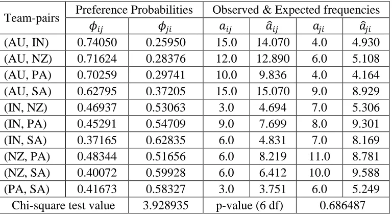
Table 2: Preference Probabilities and Observed & Expected frequencies
Team-pairs Preference Probabilities Observed & Expected frequencies
𝜙𝜙𝑖𝑖𝑖𝑖 𝜙𝜙𝑖𝑖𝑖𝑖 𝑎𝑎𝑖𝑖𝑖𝑖 𝑎𝑎�𝑖𝑖𝑖𝑖 𝑎𝑎𝑖𝑖𝑖𝑖 𝑎𝑎�𝑖𝑖𝑖𝑖
(AU, IN) 0.74050 0.25950 15.0 14.070 4.0 4.930
(AU, NZ) 0.71624 0.28376 12.0 12.890 6.0 5.108
(AU, PA) 0.70259 0.29741 10.0 9.836 4.0 4.164
(AU, SA) 0.62795 0.37205 15.0 15.070 9.0 8.929
(IN, NZ) 0.46937 0.53063 3.0 4.694 7.0 5.306
(IN, PA) 0.45291 0.54709 9.0 7.699 8.0 9.301
(IN, SA) 0.37165 0.62835 6.0 4.831 7.0 8.169
(NZ, PA) 0.48344 0.51656 6.0 8.219 11.0 8.781
(NZ, SA) 0.40072 0.59928 6.0 6.412 10.0 9.588
(PA, SA) 0.41673 0.58327 3.0 3.751 6.0 5.249
Table 3: Hyperparametric and parametric estimates
Estimates of
the dirichlet prior Teams Worth estimates
𝛼𝛼1 Australia 0.36200
𝛼𝛼2 India 0.12686
𝛼𝛼3 New Zealand 0.14342
𝛼𝛼4 Pakistan 0.15324
𝛼𝛼5 South Africa 0.21448
The chi-square test value 3.928935
p-value at 6 d.f. 0.686487
The estimates of the worth parameters show that the Kangaroos stand first, South Africans the second, Pakistanis being third, Kiwis being the fourth and finally Indians with the lowest rank. The entire estimates yield a small chi-square test value 3.928935 and the associated highly insignificant p-value 0.686487.
4. Conclusions
An elicitation technique based on the minimum chi-square approach is suggested for the estimation of hyperparameters of the prior distribution of the parameters of the PC models. The entire elicitation procedure is illustrated taking a real dataset on five ODI cricket teams. Frequentists usually object the Bayesians for the reason that they utilize subjective information collected from experts for elicitation and it makes the entire Bayesian procedures subjective. But by using MCS technique, there remains no issue of subjectivity. Having a view of the facts and figures of the analysis given in the form of posterior means, we see that the five ODI cricket teams under study may be ranked as Australia being the number one, South Africa the second one, Pakistan being the third one, New Zealand with the fourth position and finally India being the fifth and last one. It is important to know that the suggested technique can efficiently be used to elicit the hyperparameters of all types of priors.
Acknowledgements
Appendix
/* 'C' codes to elicit hyperparameters of Dirichlet prior for Chi-square model */ # include <stdio.h>
# include <math.h> # include <conio.h>
# define pi 3.141592653589793 void main()
{ inti,j;
double p_value,t1,t2,t3,t4,t5, h1,h2,h3,h4,h5,p12,p13,p14,
p15,p23,p24,p25,p34,p35,p45,p21,p31,p41,p51,p32,p42,p52,p43,p53,p54,ord, pp12,pp13,pp14,pp15,pp23,pp24,pp25,pp34,pp35,pp45,pp21,pp31,pp41,pp51,pp32, pp42,pp52,pp43,pp53,pp54,lf,prior,post,integ,integc,e[5][5],chiold=50.50,chi=0.0, chi1,pij,est[5],obs[5][5]={0,15,12,10,15,4,0,3,9,6,6,7,0,6,6,4,8,11,0,3,9,7,
10,6,0},integt1,integt2,integt3,integt4,integt5,dl=0.05; clrscr();
printf("Start of Program..."); for (h1=0.01;h1<=1.0-dl;h1+=dl) for (h2=0.01;h2<=1.0-h1-dl;h2+=dl) for (h3=0.01;h3<=1.0-h1-h2-dl;h3+=dl) for (h4=0.01;h4<=1.0-h1-h2-h3-dl;h4+=dl) {
h5=1.0-h1-h2-h3-h4;
// Finding the Normalizing Constant
integ=0.0; integt1=0.0; integt2=0.0; integt3=0.0; integt4=0.0; for (t1=0.01;t1<=1.0-dl;t1+=dl)
for (t2=0.01;t2<=1.0-t1-dl;t2+=dl) for (t3=0.01;t3<=1.0-t1-t2-dl;t3+=dl) for (t4=0.01;t4<=1.0-t1-t2-t3-dl;t4+=dl) {
t5=1.0-t1-t2-t3-t4;
p12=t1/(t1+t2); p13=t1/(t1+t3); p14=t1/(t1+t4); p15=t1/(t1+t5); p23=t2/(t2+t3); p24=t2/(t2+t4); p25=t2/(t2+t5); p34=t3/(t3+t4); p35=t3/(t3+t5); p45=t4/(t4+t5); lf=pow(p12,15)*pow(1.0-p12,4)*pow(p13,12)*pow(1.0-p13,6)*pow(p14,10)*pow(1.0-p14, 4)* pow(p15,15)*pow(1.0-p15,9)*pow(p23, 3)*pow(1.0-p23,7)*pow(p24,9)*pow(1.0-p24, 8)*pow(p25, 6)*pow(1.0-p25,7)*pow(p34, 6)*pow(1.0-p34,11)*pow(p35, 6)*pow(1.0-p35,10)* pow(p45, 3)*pow(1.0-p45,6);
prior=pow(t1,h1 -1.0)*pow(t2,h2-1.0)*pow(t3,h3-1.0)*pow(t4, h4-1.0)* pow(t5,h5-1.0); post=lf*prior;
integ+=post*pow(dl,4);
integt1+=post*t1*pow(dl,4); integt2+=post*t2*pow(dl,4); integt3+=post*t3*pow(dl,4);integt4+=post*t4*pow(dl,4); }
integt1=integt1/integ; integt2=integt2/integ; integt3=integt3/integ; integt4=integt4/integ;
integt5=1.0-integt1-integt2-integt3-integt4;
est[0]=integt1; est[1]=integt2; est[2]=integt3; est[3]=integt4; est[4]=integt5; chi1=0.0;
//Calculating the obs., expected and chi-square value for(i=0;i<=4;i++)
if (obs[i][j]==0.0||obs[j][i]==0.0) continue; pij= est[i]/(est[i]+est[j]);
e[i][j]=(obs[i][j]+obs[j][i])*pij; chi=pow((obs[i][j]-e[i][j]),2)/e[i][j]; chi1+=chi;
}
if (chi1>chiold) continue; // To proceed with the better chi-square value // Calculating p-value
p_value = 0.0;
for (t1=0.0;t1<=chi1;t1+=0.005)
p_value += 0.005*t1*t1*exp(-t1/2.0)/(2.0*8.0); // The Chi-square pdf clrscr();
printf("\nThe pref. probs\t\tObs. & est. frequencies"); printf("\nPairs\tphi(i,j)\tO(i,j)\t\tE(i,j)\t\tO(j,i)\t\tE(j,i)");
printf("\n******\t*********\t******\t\t*******\t\t******\t\t******"); for(i=0;i<=4;i++)
for (j=i;j<=4;j++) {
if (obs[i][j]==0.0||obs[j][i]==0.0) continue; pij= est[i]/(est[i]+est[j]);
e[i][j]=(obs[i][j]+obs[j][i])*pij; printf("\n(%d,%d): %8.5f",i+1,j+1,pij);
printf("\t\t%5.2g\t%14.4g\t\t%5.2g\t%14.4g", obs[i][j],e[i][j],obs[j][i],e[j][i]); }
printf("\n\nHyperparameters (Alpha_i): %g %g %g %g %g",h1,h2,h3,h4,h5);
printf("\nRespective Estimates (Theta_i) for: \nAustralia\tIndia\t\tNZ Land\t\tPakistan\tS Africa\n%8.5f\t%8.5f\t%8.5f\t%8.5f\t%8.5f",integt1,integt2,integt3,integt4,integt5); printf("\nThe chi-square test value: %10.6f \np-Value (6 df):%10.6f",chi1, 1.0-p_value); chiold=chi1;
printf("\nThe program is optimizing the estimates, please wait ..."); }
printf("\nThanks for your patience\nThe program ended, press Enter to exit..."); getch();
}
References
1. Abbas, N. and Aslam, M. (2011). Extending the Bradley-Terry model for paired comparisons to accommodate weights. Journal of Applied Statistics, 38(3), 571-580.
2. Adams, E.S. (2005). Bayesian analysis of linear dominance hierarchies. Animal
Behavior, 69, 1191-1201.
3. Aslam, M. (1995). Bayesian analysis for paired comparison data. Ph. D. Thesis, University of Wales, Aberystwyth, U.K.
4. Aslam, M. (2002). Bayesian Analysis for Paired Comparisons Models Allowing Ties and Not Allowing Ties. Pakistan Journal of Statistics 18(1), 55-69.
6. Bradley, R.A. and M.E. Terry (1952). Rank Analysis of Incomplete Block Designs: I. the Method of Paired Comparisons, Biometrika, 39, 324-345.
7. Chen, C. and Smith, T.M., (1984). A Bayes-type estimator for the Bradley–Terry model for paired comparisons. Journal of Statistical Planning and Inference, 10, 9–14.
8. David, H.A. (1988). The Method of Paired Comparisons. Second ed. Charles Griffin & Company Ltd., London.
9. Davidson, R.R., Solomon, D.L., (1973). A Bayesian approach to paired comparison experimentation. Biometrika60, 477–487.
10. Garthwaite, P. H., Kadane, J. B. and Hagan, A. O. (2005). Statistical Methods for Eliciting Probability Distributions. Journal of the American Statistical
Association100(470), 680-700.
11. Kim, D. H. and Kim, H. J. (2004). A Bayesian Approach to Paired Comparison of Several Products of Poisson Rates. Proceedings of the Autumn Conference,
Korean Statistical Society. 229 –237.
12. Kim, H. J. (2005). A Bayesian approach to paired comparison rankings based on a graphical model. Computational Statistics & Data Analysis, 48, 269–290.