A Graphical Method for Model Selection

Naveen Kumar Boiroju

Department of Statistics, Osmania University Hyderabad - 500 007, India

[email protected]

M. Krishna Reddy

Department of Statistics, Osmania University Hyderabad - 500 007, India

[email protected]

Abstract

In this paper, we present a graphical method for selection of a good model among the several competitive models for the same data set. The proposed method not only selects the model but also tests the equal prediction accuracy of the models. The results of the proposed method are compared with that of the model selection using Friedman test.

Keywords: Bootstrap method, Coefficient of determination, Friedman’s test and Loss function.

1. Introduction

Model selection among many competing models is one of the crucial jobs in regression and time series analysis. Most of these criteria attempt to find the model for which the predicted values tend to be closest to the true expected values, in some average sense. In this paper, selection of the model among several models based on their out-of-sample forecasting errors is discussed. The proposed method is a two step procedure. In first step, we test the statistical significance of the models with the overall mean and in the second step; we select a good model which has minimum measure of error. Section 2 presents various procedures of model selection. Section 3 presents a graphical method for model selection. Section 4 presents an empirical study by considering the three models with equal number of parameters. Section 5 presents the conclusion.

2. Methods for Model Selection

There are many proposed methods for model selection. Some of these techniques are presented below.

Model Selection using R2

The use of coefficient of determination, _R2 _{in model selection is a common practice in}

regression analysis and time series analysis. We have seen that maximizing _R2 _{is not a}

sensible criterion for selecting a model, because the most complicated model will have the largest _R2 _{value. This reflects that fact that R}2 _{has an upward bias as an estimator of}

the population value of _R2_{. This bias is small for large n but can be considerable with}

addition of an explanatory variable cannot cause this statistic to fall. In comparing predictive power of different models, it is often more helpful to use adjusted _R2 _instead

of _R2_{. Adjusted R}2 _{is given by}

2 2

2 ₁

y e

adj _ss

R   , where _s2 _





_yyˆ



2 /



_n



_p1





e is the

estimated conditional error variance (i.e. the mean squared error) and



 

2/ 1



2 _



_{y y n}

sy is the sample variance of y. Unlike ordinary R2, if an

explanatory variable is added to a model that is not especially useful, then 2 adj

R may even decrease. This happens when the new model has poorer predictive power, in the sense of a larger value of the mean squared error. One possible criterion for selecting a model is to choose the one having the greatest value of 2

adj

R . This is, equivalently, selection of the model with smallest mean squared error value.

Model Selection using Index of agreement (d)

The index of agreement(d) was proposed by Willmott (1981) to overcome the insensitivity of _R2 _{to differences in the observed and predicted means and variances .The}

index of agreement represents the ratio of the mean square error and the potential error (Willmot,1982) and is defined as













 













_N

t t t

N

t t t

y

y

y

y

y

y

d

1 2 1 2

ˆ

ˆ

1

₍₁₎

The potential error in the denominator represents the largest value that the squared difference of each pair can attain with the mean square error in the numerator. The range of d is similar to that of _R2 _{and lies between 0 (no agreement) and 1 (perfect agreement).}

Select the model which has maximum index of agreement.

Model Selection using Measures of Error

One method for evaluating a forecasting technique uses the summation of the absolute errors. The mean absolute error (MAE) measures forecast accuracy by averaging the magnitudes of the forecast errors (i.e. absolute values of each error). MAE is most useful when the analyst wants to measure forecast error in the same units as the original series.





     N t t N

t t t

e N y y N MAE 1 1 1 ˆ 1 ₍₂₎

And the root mean squared error (RMSE) is given as





     N t t t N t t e N y y N RMSE 1 2 2 1 1 ) ˆ ( 1 ₍₄₎

MAPE is a relative error statistic measured as average percent errors of the historical data points and is most appropriate when the cost of the forecast error is more closely related to the percentage error than the numerical size of the error. MAPE is computed as the average of the absolute percentage error values.

100 1 1  



 N t t t Z e N

MAPE . (5)

MAPE provides an indication of how large the forecast errors are in comparison to the actual values of the series. A model is said to be good if the MAPE value is not greater than five. Select the model which has minimum MAE, RMSE and MAPE values. (De Gooijer and Hyndman, 2006).

Model Selection using Percentage Better Statistic

There are several commonly used types of scale-independent statistic. The first type essentially relies on pair wise comparisons. If method A and method B, say, are tried on a number of different series, then it is possible to count the number of series where method A gives better forecasts than B (using any sensible measure of accuracy). Alternatively, each method can be compared with a standard method, such as the random walk forecast (where all forecasts equal the latest observation), and the number of times each method outperforms the standard is counted. Then the percentage number of times a method is better than a standard method can readily be found. This statistic is usually called ‘Percent Better’.

Let _*

t t t _ee

r  denote the relative error, where * t

e is the forecast error obtained from the

base method. Usually, the base method is a benchmark method or the naive method where yˆ is equal to the last observation.t

Percentage better (PB) =











n i t

n

r

I

1

1

100

_{where I(u)=1 if u is true and 0 otherwise.}

Model Selection using AIC or SBC

An approach to model selection that considers both the model fit and the number of parameters has been developed. The information criterion of Akaike or AIC, selects the best model from a group of candidate models as the one that minimizes AIC =

p n

2 ˆ

ln



2 _{ where ˆ}2 _{is the residual variance, nis the number of residuals andpis the}

number of parameters in the model.

The Bayesian information criterion developed by Schwartz or SBC, selects the model

that minimizes SBC = p

n n) ln( ˆ

ln



2 _{ . The second term in both AIC and SBC is}

penalty factor for including additional parameters in the model. Since the SBC criterion imposes a greater penalty for the number of parameters than does the AIC criterion, use of minimum SBC for model selection will result in a model whose number of parameters in no greater than that chosen by AIC. Often, the two criteria produce the same result. We select the model which has minimum of AIC and SBC values. (Akaike, 1974; Schwartz, 1978).

Model Selection using Friedman Statistic

Friedman’s test is used to compare the multiple forecasting models with respect to squared errors or absolute errors and trying to infer whether there are significant general differences in performance of the models. Friedman’s test is a nonparametric test which is designed to detect differences among two or more groups. Friedman’s test, operating on the sum of the ranksR_j, considers the null hypothesis that all models are equivalent in performance (have similar mean ranks). Under the null hypothesis, the following statistic:













 



 k

j j

F _{nk k} R n k

1 2

2 _{3 1}

1 12



₍₆₎

is approximately distributed as _2_{with k-1 degrees of freedom and where k= number of}

Model Selection using Principle of Parsimony

All things being equal, simple models are preferred to complex models. This is known as the “principle of parsimony” with a limited amount of data; it is relatively easy to find a model with a large number of parameters that fits the data well. However forecasts from such a model are likely to be poor because much of the variation in the data due to random error is modeled. The goal is to develop the simplest model that provides an adequate description of the major features of the data. The principle of parsimony refers to the preference for simple models over complex ones. (Chatfield, 1991).

3. A Graphical Method for Model Selection

In this section, we propose a graphical procedure using bootstrap method for the selection of a good model among the several competitive models. The bootstrap has been the object of much research in statistics since its introduction by Efron (1979). The bootstrap is a method for estimating the distribution of an estimator or test statistic by resampling one's data. It amounts to treating the data as if they were the population for the purpose of evaluating the distribution of interest. Under mild regularity conditions, the bootstrap yields an approximation to the distribution of an estimator or test statistic that is at least as accurate as the approximation obtained from first-order asymptotic theory. (Efron and Tibshirani, 1993).

Let the forecasting error et  yt yˆtand let



dit g

 

eit ,i 1,2,,k; t 1,2,,m



represent the tth error generated by the ith model, where m is the number of forecasts generated by the ith _{model and g}



_{. being some specified loss function, for example,}

 

e e

g  _{or g}

 

_{e e}2_org

 

_{e  e. And the mean of the error function of the i}th _{model is}





 m

t it

i _m d

d

1

1 _{. Bootstrap graphical procedure for selecting a model among the adequate}

models is given in the following steps:

1. Let



_d* ,_i1,2, .. ,._k; _j1,2, ...,_m;_b1,2, .. ,._{B }5000



bij represents the errors of

b-th bootstrap sample of size m, drawn from ithmodel.

2. Compute *

bi

d , the mean of b-th bootstrap sample form ith _{model is given by}





 m

j bij

bi _m d

d

1 *

* 1 _{, i=1,2,…,k; b=1,2,…, B.}

Compute





 k

i bi

b _k d

d

1 *

* 1 _{, b=1,2, …, B.}

3. Obtain the sampling distribution of the mean using B-bootstrap estimates and compute the central decision line (CDL) as





 B

b b

d B d

1 *

4. The lower decision line (LDL) and the upper decision line (UDL) for the comparison of each of the 2

i

s are given by:

 *m1

d

LDL (7)

 *m2

d

UDL (8)

where                              

 B B

k m B k m , 2 1 min , 2 ,1 max 2 1  

,  0.05, _{ }*

1

m

d and

 *m2

d are the _mth

1 and m2th order statistics respectively from the bootstrap

estimates * b

d , b=1, 2, …,B and [x] represents the integer part.

5. Plot di against the decision lines. If any one of the points plotted lies outside the

respective decision lines, null hypothesis of equal prediction performance of the models is rejected at  level and we may conclude that the prediction performance of the models is not same.

6. If any one of the points plotted above the UDL, then the corresponding models are considered to be inefficient models and may be eliminated from the analysis. If the points plotted below the LDL, then the corresponding models can be considered as efficient models for prediction and we select the model which is very close to the x-axis or zero. If the points falling in between the UDL and LDL then the corresponding models can be treated as equally efficient in their prediction accuracy.

This method not only tests the significant difference among the models but also identify the source of heterogeneity of models. The proposed method depends only on the supplied information and does not require any distributional assumptions.

4. Empirical Study

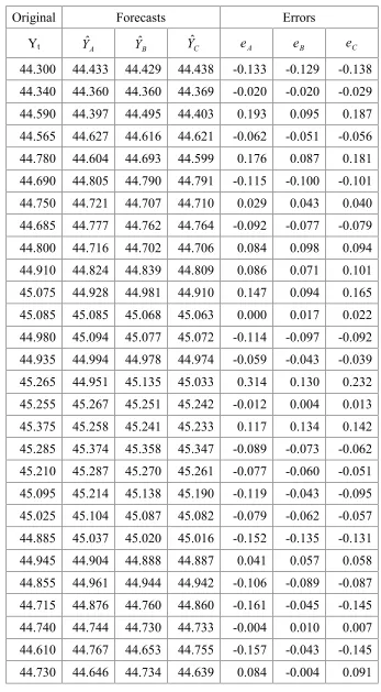
Table 1: Out-of-sample data, forecasts and errors

Original Forecasts Errors

Yt Yˆ_A Yˆ_B YˆC eA eB eC

44.300 44.433 44.429 44.438 -0.133 -0.129 -0.138

44.340 44.360 44.360 44.369 -0.020 -0.020 -0.029

44.590 44.397 44.495 44.403 0.193 0.095 0.187

44.565 44.627 44.616 44.621 -0.062 -0.051 -0.056

44.780 44.604 44.693 44.599 0.176 0.087 0.181

44.690 44.805 44.790 44.791 -0.115 -0.100 -0.101

44.750 44.721 44.707 44.710 0.029 0.043 0.040

44.685 44.777 44.762 44.764 -0.092 -0.077 -0.079

44.800 44.716 44.702 44.706 0.084 0.098 0.094

44.910 44.824 44.839 44.809 0.086 0.071 0.101

45.075 44.928 44.981 44.910 0.147 0.094 0.165

45.085 45.085 45.068 45.063 0.000 0.017 0.022

44.980 45.094 45.077 45.072 -0.114 -0.097 -0.092

44.935 44.994 44.978 44.974 -0.059 -0.043 -0.039

45.265 44.951 45.135 45.033 0.314 0.130 0.232

45.255 45.267 45.251 45.242 -0.012 0.004 0.013

45.375 45.258 45.241 45.233 0.117 0.134 0.142

45.285 45.374 45.358 45.347 -0.089 -0.073 -0.062

45.210 45.287 45.270 45.261 -0.077 -0.060 -0.051

45.095 45.214 45.138 45.190 -0.119 -0.043 -0.095

45.025 45.104 45.087 45.082 -0.079 -0.062 -0.057

44.885 45.037 45.020 45.016 -0.152 -0.135 -0.131

44.945 44.904 44.888 44.887 0.041 0.057 0.058

44.855 44.961 44.944 44.942 -0.106 -0.089 -0.087

44.715 44.876 44.760 44.860 -0.161 -0.045 -0.145

44.740 44.744 44.730 44.733 -0.004 0.010 0.007

44.610 44.767 44.653 44.755 -0.157 -0.043 -0.145

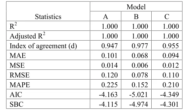
We compute the error statistics for the three models and the results are presented below. Table 2: Measures of Errors

Statistics A ModelB C

R2 _{1.000 1.000 1.000}

Adjusted R2 _{1.000 1.000 1.000}

Index of agreement (d) 0.947 0.977 0.955

MAE 0.101 0.068 0.094

MSE 0.014 0.006 0.012

RMSE 0.120 0.078 0.110

MAPE 0.225 0.152 0.210

AIC -4.163 -5.021 -4.349

SBC -4.115 -4.974 -4.301

From the above table it is clear that the model B has maximum index of agreement and minimum MAE, MSE, RMSE, MAPE, AIC and SBC values. Hence the model B is selected among the models.

The results of percentage better statistics for the selected models are presented in the following table.

Table 3: Percentage Better Performance of the Models

PB (%) Base Method

Model A B C

A - 21.43 46.43

B 78.57 - 64.29

C 53.57 35.71

-From the above table, it is observed that the model A is 21.43% and 46.43% better than the B and C models respectively. Model B is 78.57% and 64.29% better than the A and C models respectively. Model C is 53.57% and 35.71% better than the A and B models respectively. Therefore the best suitable model for forecasting is model B and which has maximum percentage better performance comparing to other models.

We apply the Freidman test considering the absolute errors of the models and their mean ranks are 2.304, 1.589 and 2.107 for the models A, B and C respectively. The following table shows the Freidman test statistic and its asymptotic significant probability.

Since the p-value is less than 0.05, therefore the null hypothesis of equal prediction performance of the models is rejected and we may conclude that the prediction performance of the models is not the same. Thus the model B is selected, since it has first rank among the models.

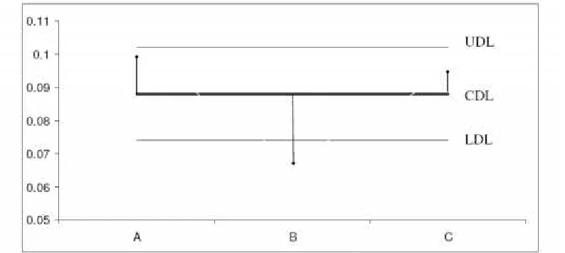
We have considered the absolute errors of the three models and the mean values obtained are d_A 0.101,d_B 0.068andd_C 0.094 for the models A, B and C respectively. By applying the bootstrap procedure explained in Section 2, the LDL, CDL and UDL are obtained as 0.074, 0.088 and 0.102 respectively. Prepare a chart as in Figure 1, with the above decision lines and plot the pointsdi



i A,B,C



. From the Figure 1, we observe that dBlie outside the decision lines. Hence, H0 may be rejected and it may be concluded

that the mean absolute errors of three forecasting models are not equal. From the same figure it is observed that dA and dC lies within the LDL and UDL, it indicates that the

prediction performance of the models A and C is same. Since the dB value lies below the

LDL, therefore the corresponding model B is selected and we may conclude that the model B is an efficient model among the models.

Figure 1: Comparison of forecasting models

5. Conclusion

References

1. AdilKorkmaz and M. BurakÖnemli (2011). Model Selection by Friedman Statistic, Pak.j.stat.oper.res., Vol.VII, No. 2-Sp 2011, 473-481.

2. Akaike, H. (1974). A new look at the statistical model identification. IEEE transactions on automatic control, 19 (6), 716-723.

3. Chatfield, C. (1991). “The Analysis of Time Series: An Introduction”, 5th _ed.,

Chapman and Hall, London.

4. De Gooijer, J.G., Hyndman, J.R. (2006). 25 Years of Time Series Forecasting, International Journal of Forecasting, 22, 443– 473.

5. Efron, B, and Tibshirani, R.J. (1993). An introduction to the bootstrap. Chapman and Hall, London.

6. Efron, B. (1979). Bootstrap methods: Another look at the Jackknife. Annals of Statistics, 7, 1-26.

7. Naveen Kumar Boiroju (2011). Forecasting Foreign Exchange Rates using Neural Networks, Unpublished Ph.D. work, Osmania University, Hyderabad.

8. Schwarz, G. (1978). Estimating the Dimension of a Model, Annals of Statistics, Vol. 6, No. 2, March, 461-464.

9. Willmott, C.J. (1981). On the Validation of Models, Physical Geography, 2, 184-194.