Linear programming control of a group of heat pumps

O R I G I N A L A R T I C L E

Open Access

Linear programming control of a group of

heat pumps

Jiˇrí Fink

, Richard P. van Leeuwen

, Johann L. Hurink

and Gerard J.M. Smit

Abstract

Background: For a new district in the Dutch city Meppel, a hybrid energy concept is developed based on bio-gas co-generation. The generated electricity is used to power domestic heat pumps which supply thermal energy for domestic hot water and space heating demand of households. In this paper, we investigate direct control of the heat pumps by the utility and how the large-scale optimization problem that is created can be reduced significantly.

Methods: Two different linear programming control methods (global MILP and time scale MILP) are presented. The latter solves large-scale optimization problems in considerably less computational time. For simulation purposes, data of household thermal demand is obtained from prediction models developed for this research. The control methods are compared with a reference control method resembling PI on/off control of each heat pump.

Results: The reference control results in a dynamic electricity consumption with many peak loads on the network, which indicates a high level of simultaneous running heat pumps at those times. Both methods of mix integer linear programming (MILP) control of the heat pumps lead to a much improved, almost flat electricity consumption profile.

Conclusions: Both optimization control methods are equally able to minimize the maximum peak consumption of electric power by the heat pumps, but the time scale MILP method requires much less computational effort. Future work is dedicated on further development of optimized control of the heat pumps and the central CHP.

Keywords: Smart grid, Linear programming control, Heat pumps, Thermal storage, Load balancing, Demand side management

Background Introduction

To reduce fossil fuel usage and increase the share of renewable energy, the Netherlands plans for 14 % renew-able energy of the total energy consumption by the year 2020 and 100 % in the year 2050 [1]. However, integra-tion of renewable energy in existing distribuintegra-tion grids may cause problems with power stability in some regions at times when there is a large amount of energy offered by solar PV installations or wind turbines and low demand [2]. Smart grids are seen as a possible solution and there-fore the Dutch government started the Topteam Energy which defined the innovation contract smart grids [3] with the following goals:

*Correspondence: [email protected]

2University of Twente, Department of Computer Science, Mathematics and Electrical Engineering, P.O. Box 217, 7500 AE, Enschede, The Netherlands Full list of author information is available at the end of the article

• reduce costs for integration of renewable energy into distribution grids

• increase consumer awareness and energy savings • contribute to a competitive energy market and

consumer choice resulting in reductions in energy prices

It is widely recognized that smart grids are required to balance energy production with loads and energy storage. This is made possible by sophisticated control strategies and communication networks.

To increase the share of renewable energy in today’s energy system, it is not always necessary to integrate the renewable energy into existing grids. With so-called smart microgrids, it is possible to connect or disconnect a region to or from the main distribution grid. In Meppel, a small city in the Netherlands, there is a plan to build a dis-trict (Nieuwveenselanden) with an energy system called MeppelEnergie[4–6] that can be defined as a smart micro-grid and which has the goal to become almost 100 %

renewable. The heart of the system is a combined heat and power (CHP) unit which is supplied with biogas from a nearby wastewater treatment facility. Part of the houses in the district are connected to the district heating system, while other houses have a heat pump. Both the heat for the district heating system and power for the heat pumps are supplied by the CHP. This is a typical case where a smart grid is required for load balancing purposes, otherwise the district would need frequent power exchanges with the existing power grid. Without a smart grid, this would probably involve large peak loads and strengthening of the existing grid would be required, involving high costs for new cabling and bi-directional transformers. For different cases in Germany involving regional solar PV generation, these effects are explained by Nykamp [2]. Therefore, the heat pumps should be scheduled in such a way that they only consume, if possible, the electricity produced by the CHP. If this is not possible, the remaining energy has to be bought on the electricity market at minimal cost.

The planning of a group of heating systems may have many objectives in practice. In the Meppel project, biogas is transported through a dedicated pipeline and electric energy is distributed through a private cable and con-verted by heating supply systems. In general, generators and transport equipment have to be dimensioned for the maximal peak consumption. Thus, the main objec-tive is minimizing the maximal consumption which may decrease investments in the system and will also lead to maximum self consumption of the generated electricity by the biogas CHP.

This paper develops a smart grid control method with the goal to minimize peak consumption. We further demonstrate the importance of this method for the Mep-pel case. After a review of related work in section “Related work”, a more detailed problem formulation which leads to an algorithm called global mix integer linear pro-gramming (MILP) control is given in section “Problem statement and global MILP control”. As this algorithm requires a lot of computational power, we develop an algo-rithm called time scale MILP control in section “Time scale MILP control”. The Meppel case is explained in section “Case application”. The simulation results are pre-sented in section “Results and discussion”. Finally, we draw conclusions in section “Conclusions”.

Related work

The problem of minimizing peak consumption of a group of heat pumps is a typical smart grid control problem. As demonstrated by Nykamp [2], integration of renewable energy (e.g., by wind turbines, solar PV, and biomass con-version) requires implementation of control strategies for load balancing and load shifting in electrical grids. This is either due to the stochastic nature of the energy produc-tion or due to supply limitaproduc-tions of the biomass. In the

Meppel case, the supply of biogas to the CHP which gen-erates the electricity for the heat pumps is limited. Besides that, the biogas supply is approximately constant in time and it is not possible to divert the biogas supply to other consumers. These are totally different circumstances than existing natural gas CHP systems. The natural gas sup-ply system is widespread within the Netherlands, and for CHP’s on natural gas, there are usually no limitations to size or consumption patterns.

For load balancing purposes, Stadler et al. [7] introduce three possible device control strategies for refrigerators which are also applicable for heat pumps.

1. Autonomous control is performed by the device itself, e.g., by sensing the grid frequency, interpreting the difference with a nominal frequency, and making decisions to start or stop the heat pump. In our case, we expect poor results from this type of control because there are also constraints on thermal comfort which are likely to create conflicts in time with reaching grid stability.

2. Price-based control is the dominating control strategy for scheduling devices within a smart grid. The heat pump determines an operational schedule based on dynamic price information which is sent to the heat pumps by the utility. However, to make a sensible decision about future schedules, it is required that a heat pump controller is able to predict future heat demand of the building. For this purpose, model predictive control is implemented within the heat pump controller. For climate control of a single building with a heat pump and

time-varying electricity prices, model predictive control is developed and demonstrated by Halvgaard et al. [8]. For groups of devices, a smart grid control strategy based on the principles of price-based control is developed within the TRIANA smart grid control methodology by Molderink [9], Bakker [10], and Bosman [11]. Bosman demonstrates the use of this type of control for a group of microCHP’s in [11], while Bakker also demonstrates results for a group of heat pumps in [10]. These examples demonstrate effectiveness of price-based control. The only minor disadvantage of price-based control is the need for an intelligent heat pump controller for each house. 3. Direct control involves making control decisions for

calculation. In the Meppel case, the number of houses with a heat pump connected to a single biogas CHP is limited to 135. For mathematical optimization, we estimate that this is a feasible challenge and that is why we chose this method for the Meppel case.

The mathematical background of the minimizing peak problem is presented in [12] which proves that the prob-lem of minimizing peak is NP-complete. A somewhat similar problem was considered by Bosman et al. [13, 14] who studied a microCHP planning problem and also proved that minimizing peak is NP-complete in their model [15]. Bosman et al. [11] also present a dynamic pro-gramming algorithm for the microCHP planning prob-lem whose time complexity is O(T3C+1) where T is the number of time intervals and C is the number of microCHPs.

The main contribution of this paper is that we demon-strate by development of the time scale control method and the application within the Meppel case that the num-ber of variables and equations which are part of the large-scale optimization problem on the utility level can be reduced considerably while the control objective of minimizing the peak consumption is still reached.

Methods

Problem statement and global MILP control

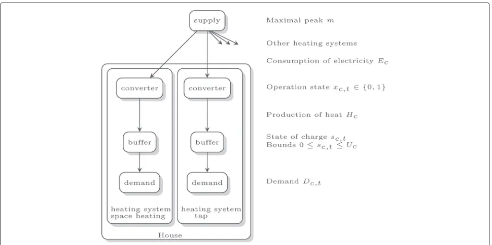
In this section, we present a mathematical description of the studied model and possible applications of this model. The model is set up to be generally applicable for any type of heating appliance. Typical appliances for heating water are electrical and gas heating systems, heat pumps, and combined heat and power units (microCHP). The heated water is stored in buffers to be prepared for the demand of inhabitants. In our model, a house consists of two local heating systems, one for space heating and the other for tap. A schematic overview of the model is presented in Fig. 1. It consists of:

• a supply which represents some source of energy (e.g., electricity, gas),

• a converter which converts the energy into heat (hot water),

• a buffer which stores heat for later usage, and • a demand which represents the consumption profile

of heat.

In principle, the presented model can consider arbitrary types of energy but in this paper, we use electricityand heatto distinguish consumed and produced energy. This simple model of a local heating system cannot only be applied for heating water but has many other applications in smart grids (e.g., control of fridges and freezers) and inventory management. We come back on this at the end of this section.

We consider a discrete time model for the considered problem, meaning that we split the planning period into T time intervals of the same length. We consider a set

C = {1,. . .,C} of C heating systems and a set

T = {1,. . .,T}ofT time intervals. Note that the heating of a house is split into two independent heating systems (see Fig. 1). In this paper, the lettercis always an index of a heating system (either space heating or tap) andtis an index of a time interval. For mathematical purposes, we separate a heating system into a converter, a buffer, and demand; see Fig. 1. We say “a converterc,” “a bufferc,” or “a demandc” to refer to the devices of the heating system c∈C.

We consider a simple converter which has only two states: In every time interval, the converter is either turned on or turned off. The amount of consumed electricity is Ecand the amount of produced heat (or any other form of

energy) isHcduring one time interval in which the

con-verterc ∈ C is turned on. If the converter is turned off, then it consumes and produces no energy. Letxc,t∈ {0, 1}

be the variable indicating whether the converterc ∈ Cis running in time intervalt∈T.

The state of charge of a bufferc∈Cat the beginning of time intervalt∈T is denoted bysc,twhich represents the

amount of heat in the buffer. Note thatsc,T+1is the state of

charge at the end of planning period. The state of charge sc,tis limited by an upper boundUc.

The amount of consumed heat by the inhabitants of the house from heating system c ∈ C during time interval t ∈ T is denoted byDc,t. This amount is assumed to be

given and is called the demand of heating systemc. In this paper, we study offline problems, so we assume that demandsDc,tare given for the whole planning period.

The operational variables of the converters xc,t and

the states of charge of buffers sc,t are restricted by the

following constraints.

sc,t+1=sc,t+Hcxc,t−Dc,tforc∈C,t∈T (1)

0≤sc,t≤Ucforc∈C,t∈{1,. . .,T+1}(2)

xc,t∈ {0, 1} forc∈C,t∈T (3)

Equation 1 is the charging equation of the buffer. During time intervalt∈T, the state of chargesc,tof a bufferc∈C

is increased by the production of the converter which is Hcxc,tand it is decreased by the demandDc,t. Equations (2)

and (3) ensure that the domains of variablessc,tandxc,t,

respectively, are taken into account. Note that the initial state of chargesc,1can be fixed (e.g., by settingsc,1= U₂c).

In this paper, we consider the objective function of minimizing the peak:

minimize m

Fig. 1Schematic picture of a house with two separated heating systems for space heating and tap

SinceEcxc,tis the amount of consumed electricity by a

convertercin time intervalt, the sum_c∈CEcxc,tis the

amount of electricity consumed by all converters in time intervalt. Furthermore, the inequality and the objective function (4) guarantees that the value of the variablemis the maximal consumption of electricity during one time period within the whole planning period.

In the following, we give some other possible applica-tions of this model.

Fridges and freezers: A fridge essentially works in the opposite way than heating, so it may be modelled sim-ilarly. However, we have to be careful with the correct interpretation of all parameters. The state of charge of the buffer again represents the temperature inside the fridge, but a higher state of charge means a lower temperature. The converter does not produce heat to the fridge but it decreases the temperature inside the fridge, so the con-verter increases the state of charge of the buffer (fridge). The demand decreases the state of charge of the fridge due to thermal loss and usage of the fridge by humans.

Inventory: The considered heating problem is also related to inventory control problems [16]. A buffer may represent an inventory and a converter may represent orders. However, this leads to a situation, where only a limited capacity of inventory is given and it is only possi-ble to order a fix amount of goods which is not a typical situation in inventory management.

Note that the objective function and all constrains are linear and operational state variables are binary, so con-straints and the objective (1)–(4) form an instance of MILP. This instance can be solved by any MILP solver

(see, e.g., [17]) and we call this approach global MILP control. However, as the number of binary variables may get too large for planning many houses over a long planning horizon, this method may get computationally expensive. Therefore, in the following sections, an algo-rithm which significantly reduces the number of variables is given.

Time scale MILP control

The method presented in the previous section creates one large instance of MILP and solves it by a MILP solver. This method gives us an optimal solution for the whole planning period but it may not be suitable for practical purposes. First, finding an optimal solution requires a lot of computational power. Next, the prediction of demand for the distant future may be very inaccurate.

Therefore, we consider an online control in which the decision which converters will be running is made only for the coming time interval. On the other hand, we cannot ignore the future completely. Indeed, we should take more care about the near future time intervals than the distant ones because the current decision has stronger impact on the near future and the prediction is in general more accurate for the near future.

As the general formal notation of time scale control may be hard to understand, we use an example to present the approach. Assume that the upcoming time interval has index 1. The decision which converters c ∈ C will be running during the coming time interval 1 needs to be made, meaning that the values of variablesxc,1 need

future needs to be detailed, we also consider binary vari-ables, e.g., for the next two time intervals, i.e., variables xc,2andxc,3. For the further future, the plan does not need

to be so precise, so ,e.g., another two time intervals, we relax the integral constraints, meaning that we require 0≤xc,4,xc,5≤1. The reason for relaxing these variables is

to decrease the number of integral variables which has the dominating effect on the computational time required to solve an MILP instance. From the practical point of view, these relaxed variables (e.g.,xc,4) can signify the

probabil-ity that a converter cwill run in time interval 4, and so

c∈CHcxc,4is the expected demand of electricity.

Following this, for the even more distant future, we only need a rough planning. In order to explain the idea of rough planning, let us consider the state of charge equation, e.g., for time intervalst=8, 9 and 10.

sc,9 = sc,8+Hcxc,8−Dc,8

sc,10 = sc,9+Hcxc,9−Dc,9

sc,11 = sc,10+Hcxc,10−Dc,10 (5)

We sum these equations and after simplification, we obtain

sc,11=sc,8+Hc(xc,8+xc,9+xc,10)−(Dc,8+Dc,9+Dc,10)

(6)

The rough plan for converter c for time intervals t,t+1,. . .,tis now defined byxc,t..t =t

i=txc,i, that is we

replace time intervalst,t+1,. . .,tby one block of time intervals t..t. During this block, converter c consumes Ecxc,t..t electricity and producesHcxc,t..t heat. Using this

notation, the state of charge equation for a block 8..10 of time intervalst=8, 9 and 10 is

sc,11=sc,8+Hcxc,8..10−Dc,8..10 (7)

where Dc,8..10 = Dc,8 + Dc,9 + Dc,10 is the cumulative

demand for time intervals 8,9 and 10. In this example, we replace the three variablesxc,8, xc,9, andxc,10 by one

aggregated variablexc,8..10which is constrained by bounds

0 ≤ xc,8..10 ≤ 3. In this way, we can cover a longer

plan-ning horizon without requiring too many variables in an MILP instance. Furthermore, note that only the sum of demandsDc,8..10for distant future time intervals is

impor-tant. The practical consequence is that the time where a significant demand occurs does not have to be predicted precisely, e.g., in the morning, it is sufficient to predict the amount of hot water demand for evening showers but the exact time when inhabitants will take a shower can be approximated.

In our example, we consider rough planning variables xc,6..7, xc,8..10, and x11..15. In summary, all state of charge

equations are

sc,t+1 = sc,t+Hcxc,t−Dc,t for t=1,. . ., 5

sc,8 = sc,6+Hcxc,6..7−Dc,6..7

sc,11 = sc,8+Hcxc,8..10−Dc,8..10

sc,16 = sc,11+Hcxc,11..15−Dc,11..15 (8)

for everyc∈C.

The capacity constraints of buffers remain the same, so

Lc,t≤sc,t≤Uc,t for t∈ {1, 2, 3, 4, 5, 6, 8, 11, 16} (9)

The operational constraints of converters now are

xc,t ∈ {0, 1} fort∈ {1, 2, 3}

0≤ xc,t ≤1 fort∈ {4, 5}

0≤ xc,6..7 ≤2

0≤ xc,8..10 ≤3

0≤ xc,11..15 ≤5

and the objective is

minimizem

where m ≥ _c∈CEcxc,t fort∈ {1, 2, 3, 4, 5}

2m ≥ _c∈CEcxc,6..7

3m ≥ _c∈CEcxc,8..10

5m ≥ _c∈CEcxc,11..15

This instance of MILP problem can be solved by any MILP solver. The values of variables xc,1 of an optimal

solution are used to determine which convertersc ∈ C should run in the coming time interval 1. For the next time interval 2, a similar instance of an MILP problem is created by shifting indices of time intervals by one and refining the predicted demandsDc,t.

There is no general rule how time intervals should be split into blocks since it is strongly influenced by the par-ticular case studies. In this study, we use one specific choice to study the potential of this approach.

Case application

Both methods of direct control (global and time scale MILP control) are applied to a specific case involving 135 houses of the Meppel project. Each house is equipped with two heat pumps, one for domestic hot water and one for space heating. The applied energy system in Meppel is explained in detail in [18]. For the present paper, we investigate the quality of load balancing of heat pump elec-tricity demand. We compare both types of direct control with results of reference PI control that is determined by each heat pump by itself, based on signals from house and storage thermostats. To generate heat demand profiles, the following approach is followed:

• develop a thermal model to determine house space heating demand

• define various typical house and household profiles to generate a variety of space heating and domestic hot water demand profiles

• simulate space heating demand of the various households

• determine reference PI control results

• input domestic hot water and space heating demands into the global and time scale MILP control

algorithms and determine results

In the next sections, the individual steps of the approach are explained in more details.

Space heating thermal model

Suitable methods to determine space heating demand are listed in [19] and include modelling of thermal network, radiant time series, and transfer function methods. In the following, we develop a so-called grey-box model, i.e., a simplified model of a house based on the thermal network approach. An advantage of this approach is that dynamic heat demand of a house is described by only a few dif-ferential equations which are easy to integrate into smart grid control algorithms. However, model parameters may not correlate very well with true physical characteristics of the concerned building. For the purpose of the present paper, absolute accuracy of the space heating demand model is of less importance, hence we determined model parameters by physical estimation and not, e.g., by apply-ing identification techniques usapply-ing simulated or measured data. Validation of accuracy of the applied space heating demand model is part of our future work. The thermal network representation of the simplified model is shown in Fig. 2. For the indoor part, the model contains lumped thermal masses for the interior zone and floor structure. We assume an air-based heating system which gives heat-ing input directly into the zone. Towards the exterior, there are two lumped thermal masses, one for the interior walls and one for the exterior walls of the house enve-lope. The main heat loss contributions to the ambient are through the envelope walls, windows, and roof.

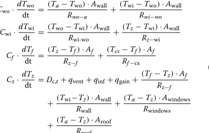
The model equations are formulated as follows:

Cwo·dTwo dt =

(Ta−Two)·Awall

Rwo−a +

(Twi−Two)·Awall

Rwi−wo

Cwi·

dTwi dt =

(Two−Twi)·Awall

Rwi-wo +

(Tz−Twi)·Awall

Rz−wi

Cf ·

dTf dt =

(Tz−Tf)·Af

Rz−f +

(Tcs−Tf)·Af

Rf−cs

Cz·

dTz

dt =Dc,t+qvent+qinf+qgain+

(Tf −Tz)·Af

Rz−f

+(Twi−Tz)·Awall

Rwall +

(Ta−Tz)·Awindows

Rwindows

+(Ta−Tz)·Aroof

Rroof

(10)

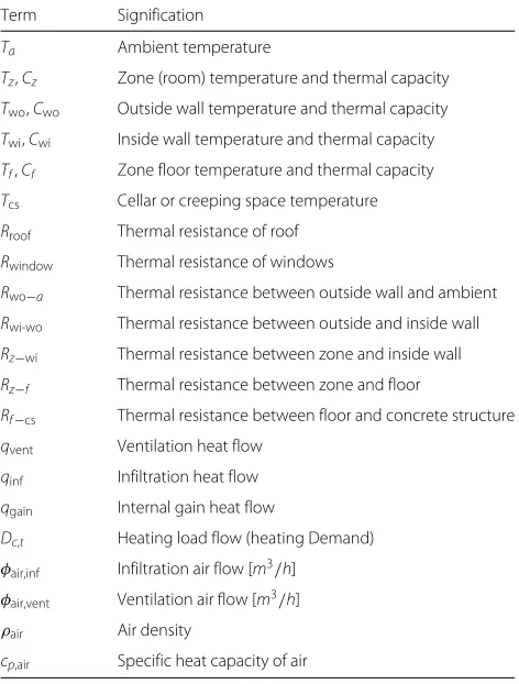
The terms in these equations are explained in Table 1. Besides heat loss to the ambient, infiltration-and ventilation-associated heat losses (qinfandqvent) are

determined by the following equations:

qinf=φair,inf·ρair·cp,air·(Ta−Tz)

qvent=φair,vent·ρair·cp,air·(Ta−Tz)·(1−γhr) (11)

The used terms are also explained in Table 1. Ventilation air flow valuesφair,ventinm3/hare defined by schedules

given in section “House and household case information”. Infiltration air flowsφair,infare related to leakages of the

building and are assumed as constant values. We defined some variations including heat recovery ventilation with a certain heat recovery efficiencyγhr.

Besides heat losses, there are scheduled heat gains (qgain) due to resident and electric appliance dissipations.

The applied schedule is given in section “House and household case information”. For the present paper, solar energy absorbed by the interior is neglected because we study a relatively cold and cloudy week.

The heat demandDc,tis calculated by solving the model

equations including a simple zone temperature control. For this, setpoint schedules for the zone temperature are defined in section “House and household case informa-tion”. The demandDc,tfor every housecand time interval

tis determined by the following rules:

• If the zone temperatureTzequals the setpoint, then

the demandDc,tis the amount of energy which the

heating system has to generate to keep the zone temperature constant.

• If the setpoint is increased, then the demandDc,tis

increased to raise the zone temperature in a given warmup speeddTz

dt.

• If the zone temperatureTzis above the setpoint (e.g.,

due to decreasing the setpoint or natural heating by internal gains), the demandDc,tis the minimal

non-negative amount of energy which keeps the zone temperature above the setpoint.

Application of weather data

Fig. 2Applied thermal network model

House and household case information

We consider a total of 135 households and we define three types of households (see Table 2) living in semi-detached and detached houses. Houses will be built in three con-struction phases and later phases will have a better ther-mal insulation due to tightening regulations. In this study, we assume that in each phase, 30 semi-detached and 15 detached houses will be built. Rc values of semi-detached houses in the respective construction phases are 3.5, 5.0, and 7.5m2K/Wand the Rc values of detached houses are 5.0, 7.5, and 10.0m2K/W.

Table 1Nomenclature energy system characterization

Term Signification

Ta Ambient temperature

Tz,Cz Zone (room) temperature and thermal capacity

Two,Cwo Outside wall temperature and thermal capacity

Twi,Cwi Inside wall temperature and thermal capacity

T_f,C_f Zone floor temperature and thermal capacity

Tcs Cellar or creeping space temperature

R_roof Thermal resistance of roof

Rwindow Thermal resistance of windows

Rwo−a Thermal resistance between outside wall and ambient

Rwi-wo Thermal resistance between outside and inside wall

Rz−wi Thermal resistance between zone and inside wall

Rz−f Thermal resistance between zone and floor

Rf−cs Thermal resistance between floor and concrete structure

qvent Ventilation heat flow

qinf Infiltration heat flow

qgain Internal gain heat flow

Dc,t Heating load flow (heating Demand)

φair,inf Infiltration air flow [m3_/h] φair,vent Ventilation air flow [m3_/h]

ρair Air density

cp,air Specific heat capacity of air

We define a lower setpoint for the zone temperature (18 ◦C) during working hours and night and a higher setpoint temperature (20◦C) otherwise. We also define domestic hot water demand for morning, afternoon, and evening peaks. See Table 2 for schedules of the tempera-ture setpoints and energy demands for hot water.

Simulation results of heating demand

The model equations given in section “Space heating thermal model” are solved using a 15-min time step which is required as a minimum time step for controlling the thermal storage and to calculate heat pump operation times. To obtain 15-min weather data, we applied linear interpolation of the 1-h data values.

We assume a heat pump coefficient of performance (COP) of 4.5 for space heating and 2.5 for domestic hot water generation during the simulation. With that, we obtain as average electricity input 116.4 kW for space heating and 19.3 kW for domestic hot water, leading to 135.7 kW total average electricity demand. If the MILP control performs well on minimizing peaks, we expect control schedules for the heat pumps to give results close to this average electricity demand.

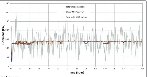
Results and discussion

In Fig. 3, we show the total electric energy consumption of the three methods of control (reference control, global MILP control, and time scale MILP control). The ref-erence control, which resembles PI control, results in a dynamic electricity consumption with many peak loads on the network, which indicates a high level of simultaneous running heat pumps at those times.

Table 2Types of households, the number of household types in both types of houses, schedules of higher temperature setting, and hot water demands

Type of household Young couple Young family Elderly people

Number of persons in a household 2 4 2

Number of houses semi-detached 27 54 9

detached 12 27 6

Higher setpoint weekdays 17–22 8–22 10–23

weekend 9–23 9–23 10–23

Hot water on weekdays morning 15 MJ 8 MJ 4 MJ

afternoon 0 MJ 4 MJ 4 MJ

evening 20 MJ 24 MJ 20 MJ

Hot water on weekend morning 8 MJ 4 MJ 4 MJ

afternoon 4 MJ 4 MJ 4 MJ

evening 24 MJ 32 MJ 24 MJ

If we consider this almost equal performance and take into account the much reduced computational effort of time scale MILP control, we prefer this method for future algorithm development.

The energy system described in section “Introduction” contains a central CHP. The obtained flat electricity demand profile of the heat pumps may be generated entirely by the central CHP but this depends on the pos-sibility to simultaneously store or use the produced heat by the CHP in a connected district heating system. Part of future work is to study possible CHP control schemes more closely, focusing on stable CHP operation, optimal

sustainability, and optimal profitability in relation to vary-ing external grid prices.

Another important quality aspect of the heat pump operation schedules obtained from the optimized con-trol is the experienced thermal comfort within the houses. This is influenced by the upper bound Uc of the state

of charge sc,t (Eq. (3)). In Fig. 4, we show the total

electric energy consumption of the heat pumps sorted from highest to lowest consumption. The MILP control results in a more horizontal distribution than the ref-erence control. In fact, depending on the value of the upper bound Uc, a whole continuum of slopes between

Fig. 4Sorted case results

the slope of the reference control and MILP control is possible. For the reference control, the value of Uc is

approximately zero, i.e., the interior temperature equals the defined setpoints in time, except for the warming up and cooling down times when the setpoint is increased or decreased from a previous state. During those times, the interior temperature needs some time to change due to thermal mass effects within the house. Part of our future research is to investigate the quality of the inte-rior temperature in relation to the value of the upper boundUc.

Conclusions

In this paper, we investigate how well a group of heat pumps for 135 different households can be controlled to minimize peaks within the electricity distribution net-work by two methods of direct control. The significance of this research is that this type of control enables integration of renewable energy within a microelectricity grid. With-out this control, power consumption peaks would occur frequently and this results into higher investments needed for network strengthening.

From simulations with a simplified thermal network model of the houses, we obtained heat demand data for space heating. For the simulations, we defined occu-pancy schedules and different insulation properties of the houses. We also defined domestic hot water demand pro-files for three types of households. We compare the total electricity consumption of all the heat pumps for the following control methods: reference (PI) control where each heat pump determines itself when to switch on or

off, and two forms of direct control: global MILP control and time scale MILP control. The latter has the advan-tage of a much reduced scale for solving the optimization problem.

In the defined case of 135 houses, MILP control decreases electricity peaks by 96 % compared to refer-ence control. The differrefer-ence between global and time scale MILP control is small. As time scale MILP control is computationally much more efficient, we propose to use time scale MILP control. The influence of the cho-sen time scaling on computational time and the quality of the achieved result is part of future work. Although the results look promising, due to the high level of peak reduction, future work will be dedicated to investigate the resulting thermal comfort as a result of the obtained heat pump planning. Also part of future work is to inves-tigate methods of reaching social fairness in heat pump planning and integrating this work into the TRIANA smart grid control method [21] to investigate possible CHP control schemes with a focus on stability, sustainabil-ity, and profitability in relation to varying electricity grid prices.

Competing interests

The authors declare that they have no competing interests.

Authors’ contributions

Authors’ information

Jiˇrí Fink was affiliated to the STW project i-Care 11854.

Acknowledgements

The authors would like to thank the Dutch national program

TKI-Switch2SmartGrids for supporting the project Meppelenergy and the STW organization for supporting the project i-Care 11854.

Author details

1_{Saxion University of Applied Sciences, Sustainable Energy Group, P.O. Box}

70.000, 7500 KB, Enschede, The Netherlands.2_{University of Twente,} Department of Computer Science, Mathematics and Electrical Engineering, P.O. Box 217, 7500 AE, Enschede, The Netherlands.

Received: 23 February 2015 Accepted: 14 October 2015

References

1. Meer Duurzame Energie in de Toekomst. visited October 2014. http:// www.rijksoverheid.nl/onderwerpen/duurzame-energie/meer-duurzame-energie-in-de-toekomst. Accessed 26 Oct 2015

2. Nykamp S (2012) Integrating renewables in distribution grids—storage, regulation and the interaction of different stakeholders in future grids. PhD thesis, University of Twente (2013). doi:10.3990/1.9789036500579 3. Innovation Contract Smart Grids. visited October 2014. http://

topsectorenergie.nl/wp-content/uploads/2013/10/InnovatieContract-Smart-Grids-2012.pdf. Accessed 26 Oct 2015

4. Nieuwveense Landen. visited March 2014. http://www.meppelwoont.nl/ nieuwveense-landen/. Accessed 26 Oct 2015

5. RVO Meppel heats new housing development with biogas. visited March 2014 (2012) http://www.rvo.nl/sites/default/files/Meppel%20heats %20new%20housing%20development%20with%20biogas.pdf. Accessed 26 Oct 2015

6. Meppel Energie. visited March 2014. http://www.meppelenergie.nl/ nieuwveense-landen. Accessed 26 Oct 2015

7. Stadler M, Krause W, Sonnenschein M, Vogel U (2009) Modelling and evaluation of control schemes for enhancing load shift of electricity demand for cooling devices. Environ Modelling & Softw 24(2):285–295 8. Halvgaard R, Poulsen NK, Madsen H, Jorgensen JB Economic model

predictive control for building climate control in a smart grid. Proceedings of 2012 IEEE PES innovative Smart Grid Technologies (ISGT) 9. Molderink A (2011) On the three step methodology for smart grids. PhD

thesis, University of Twente. doi:10.3990/1.9789036531702 10. Bakker V (2011) Triana: A control strategy for smart grids: forecasting,

planning and real-time control. PhD thesis, University of Twente. doi:10.3990/1.9789036533140

11. Bosman M (2012) Planning in smart grids. PhD thesis, University of Twente. doi:10.3990/1.9789036533867

12. Fink J, Hurink JL (2015) Minimizing costs is easier than minimizing peaks when supplying the heat demand of a group of houses. Eur J Oper Res 242:644–650

13. Bosman MGC, Bakker V, Molderink A, Hurink JL, Smit GJM (2009) The microCHP scheduling problem. In: Proceedings of the Second Global Conference on Power Control and Optimization, PCO 2009, Bali, Indonesia. AIP Conference Proceedings Vol. 1159. pp 268–275 14. Bosman MGC, Bakker V, Molderink A, Hurink JL, Smit GJM (2011)

Controlling a group of microCHPs: planning and realization. In: First International Conference on Smart Grids, Green Communications and IT Energy-aware Technologies, ENERGY 2011, Venice, Italy. pp 179–184 15. Bosman MGC, Bakker V, Molderink A, Hurink JL, Smit GJM (2010) On the

microCHP scheduling problem. In: Proceedings of the 3rd Global Conference on Power Control and Optimization PCO, 2010, Gold Coast, Australia. AIP Conference Proceedings Vol. 1239. pp 367–374

16. Axsäter S (2006) Inventory control. International series in operations research and management Science, Vol. 90. Springer, New York 17. Cook WJ, Cunningham WH, Pulleyblank WR, Schrijver A (2011)

Combinatorial optimization, Vol. 33. Wiley. com, Rhode Island 18. van Leeuwen RP, Fink J, de Wit JB, Smit GJ (2015) Upscaling a district

heating system based on biogas cogeneration and heat pumps. Energy, Sustainability Soc 5(1):16. doi:10.1186/s13705-015-0044-x

19. Mitchel JW, Braun JE (2013) Principles of heating, ventilation, and air conditioning in buildings. Wiley, New York

20. KNMI weather records station Hoogeveen. http://www.knmi.nl. Accessed 26 Oct 2015

21. Toersche HA, Bakker V, Molderink A, Nykamp S, Hurink JL, Smit GJM (2012) Controlling the heating mode of heat pumps with the TRIANA three step methodology. In: Innovative Smart Grid Technologies (ISGT), 2012 IEEE PES. pp 1–7. http://ieeexplore.ieee.org/iel5/6170475/6175527/ 06175662.pdf

Submit your manuscript to a

journal and benefi t from:

7 Convenient online submission

7 Rigorous peer review

7 Immediate publication on acceptance

7 Open access: articles freely available online

7 High visibility within the fi eld

7 Retaining the copyright to your article