RESEARCH
Pareto optimization in algebraic
dynamic programming
Cédric Saule
*and Robert Giegerich
Abstract
Pareto optimization combines independent objectives by computing the Pareto front of its search space, defined as the set of all solutions for which no other candidate solution scores better under all objectives. This gives, in a precise sense, better information than an artificial amalgamation of different scores into a single objective, but is more costly to compute. Pareto optimization naturally occurs with genetic algorithms, albeit in a heuristic fashion. Non-heuristic Pareto optimization so far has been used only with a few applications in bioinformatics. We study exact Pareto optimization for two objectives in a dynamic programming framework. We define a binary Pareto product operator ∗Par on arbitrary scoring schemes. Independent of a particular algorithm, we prove that for two scoring schemes A
and B used in dynamic programming, the scoring scheme A∗ParB correctly performs Pareto optimization over the
same search space. We study different implementations of the Pareto operator with respect to their asymptotic and empirical efficiency. Without artificial amalgamation of objectives, and with no heuristics involved, Pareto optimiza-tion is faster than computing the same number of answers separately for each objective. For RNA structure predicoptimiza-tion under the minimum free energy versus the maximum expected accuracy model, we show that the empirical size of the Pareto front remains within reasonable bounds. Pareto optimization lends itself to the comparative investigation of the behavior of two alternative scoring schemes for the same purpose. For the above scoring schemes, we observe that the Pareto front can be seen as a composition of a few macrostates, each consisting of several microstates that differ in the same limited way. We also study the relationship between abstract shape analysis and the Pareto front, and find that they extract information of a different nature from the folding space and can be meaningfully combined.
Keywords: Pareto optimization, Dynamic programming, Algebraic dynamic programming, RNA structure, Sankoff algorithm
© 2015 Saule and Giegerich. This article is distributed under the terms of the Creative Commons Attribution 4.0 International License (http://creativecommons.org/licenses/by/4.0/), which permits unrestricted use, distribution, and reproduction in any medium, provided you give appropriate credit to the original author(s) and the source, provide a link to the Creative Commons license, and indicate if changes were made. The Creative Commons Public Domain Dedication waiver (http://creativecommons. org/publicdomain/zero/1.0/) applies to the data made available in this article, unless otherwise stated.
Background
In combinatorial optimization, we evaluate a search space X of solution candidates by means of an objec-tive function ψ. Generated from some input data of size n, the search space X is typically discrete and has size O(αn) for some α. Conceptually, as well as in prac-tice, it is convenient to formulate the objective function as the composition of a choice functionϕ and a scoring function σ, ψ =ϕ◦σ, computing their composition as (ϕ◦σ )(X)=ϕ({σ (x)|x∈X}) for the overall solution. The most common form of the objective function ψ is
that σ evaluates each candidate to a score (or cost) value, and ϕ chooses the candidate which maximizes (or mini-mizes) this value. One or all optimal solutions can be returned, and with little difficulty, we can also define ϕ to compute all candidates within a threshold of optimal-ity. This scenario is the prototypical case we will base our discussion on. However, it should not go unmentioned that there are other, useful types of “choice” functions besides maximization or minimization, such as comput-ing score sums, full enumeration of the search space, or stochastic sampling from it.
Multi-objective optimization arises when we have sev-eral criteria to evaluate our search space. Scanning the pizza space of our home town, we may be looking for the largest pizza, the cheapest, or the vegetarian pizza with
Open Access
*Correspondence: [email protected]
the richest set of toppings. When we use these criteria in combination, the question arises exactly how we combine them.
Let us consider two objective functions ψ1=ϕ1◦σ1 and ψ2=ϕ2◦σ2 on the search space X and let us define different variants of an operator ∗ to designate particular techniques of combining the two objective functions.
• Additive combination(ψ1 ∗+ ψ2) optimizes over the sum of the candidates scores computed by ϕ1 and ϕ2. This is a natural thing to do when the two scores are of the same type, and optimization goes in the same direction, i.e. ϕ1=ϕ2=:ϕ; we define
In fact, this recasts the problem in the form of a single objective problem with a combined scoring function. This applies, e.g. for real costs (money), which sum up in the end no matter where they come from. Gotoh’s algorithm for sequence alignment under an affine gap model can be seen as an instance of this combination [1]. It minimizes the score sum of character matches, gap openings and gap extensions. Jumping alignments are another example [2]. They align a sequence to a multiple sequence alignment. The alignment always chooses the alignment row that fits best, but charges a cost for jumping to another row. Jump cost and regular alignment scores are balanced based on test data. However, often it is not clear how scores should be combined, and researchers resort to more general combinations.
• Parametrized additive combination (ψ1 ∗+ψ2) is defined as
Here the extra parameter signals that there is some-thing artificial in the additive combination of scores, and the is to be trained from data in different appli-cation scenarios, or left as a choice to the user of the approach. Such functions are often used in bioinfor-matics [3–7]. For example, the Sankoff algorithm scores joint RNA sequence alignment and folding by a combination of base pairing (ψ1) and sequence alignment (ψ2) score [3]. RNAalifold scores consen-sus structures by a combination of free energy (σ1) and covariance (σ2) scores [8]. Covariance scores are converted into “pseudo-energies”, and the parameter controls the relative influence of the two score com-ponents. This combination often works well in prac-tice, but a pragmatic smell remains. Returning to our earlier pizza space example: It does not really make sense to add the number of toppings to the size of the pizza, or subtract it from the price, no matter how we (1)
ψ1 ∗+ ψ2=ϕ◦(σ1+σ2).
(2)
ψ1 ∗+ψ2=ϕ◦(σ1+(1−)σ2), 0≤≤1.
choose . In a way, the parameter manifests our dis-comfort with this situation.
• Lexicographic combination (ψ1 ∗lex ψ2) performs
optimization on pairs of scores of potentially differ-ent type, not to be combined into a single score.
where (ϕ1,ϕ2) optimizes lexicographically on the
score pairs (σ1(x),σ2(x)). With the lexicographic
com-bination, we define a primary and a secondary objec-tive, seeking either the largest among the cheapest pizzas, or the cheapest among the largest—certainly with different outcomes. This is very useful, for exam-ple, when ϕ1 produces a large number of co-optimal solutions. Having a secondary criterion choose from the co-optimals is preferable to returning an arbitrary optimal solution under the first objective, maybe even unaware that there were alternatives.
Lexicographic and parameterized additive combina-tion are incomparable with respect to their scope. ∗lex can combine scoring schemes of different types, but cannot optimize a sum of two scores even when they have the same type. ∗+ does exactly this. Only when both scores have the same type, there may be a choice of big enough such that ∗+ emulates ∗lex.
• Pareto combination(ψ1∗Parψ2) must be used in the
case when there is no meaningful way to combine or prioritize the two objectives. It may also be useful and more informative in the previous scenarios, pro-ducing a set of “optima” and letting the user decide the balance between the two objectives a posteriori.
Pareto optimality is defined via (non-)domination. An element (a,b)∈(A×B)dominates another one, if it is
strictly better in one dimension, and not worse in the other. The solution set one computes is the Pareto front
of {(σ1(x),σ2(x))|x∈X}. Taking ϕ1 and ϕ2 as maximiza-tion, the Pareto front operator pf is defined on subsets S of A×B, ordered by >A and >B, respectively, as follows:
A set without dominated elements is called a Pareto set. Naturally, every subset of a Pareto set is a Pareto set, too. We define the Pareto combination as
The Pareto combination ∗Paris more general than both ∗+ and ∗lex. This is obvious for ∗lex, and is also obvious for ∗+ when the two scores are of different type. It even holds for ∗+ when they have the same type, but becomes more sub-tle. It can be shown that ∗Par produces all optima that can
(3) (ψ1∗lex ψ2)(X)=(ϕ1,ϕ2)({(σ1(x),σ2(x))|x∈X}),
(4)
pf(S)= {(a,b)∈S| � ∃(a′,b′)∈S\{(a,b)}
such that(a′,b′)dominates(a,b)}.
(5)
be produced by ∗+ for some , but there can also be others. See Theorem 3.1, and we also refer the reader to the careful treatment of this intriguing issue in Schnattinger’s thesis [9].
The combinations ∗+ and ∗+ are common practice and merit no theoretical investigation, as they reduce the problem to the single objective case. The lexicographic combination ∗lex has been studied in detail in [10]. Aside from its obvious use with primary and secondary objec-tives, ∗lex has an amazing variety of applications when of one the two objectives does not perform optimization, but enumeration or summation (cf. above). Furthermore, when σ1 computes a classification attribute from the can-didates and ϕ1 is the identity, it gives rise to the method of classified dynamic programming used, e.g. in probabil-istic RNA shape analysis [11].
Here, we will take a deeper look into Pareto optimi-zation, which has been used in bioinformatics mainly in a heuristic fashion. It naturally arises with the use of genetic algorithms. They traverse the search space improving candidates in a certain dimension, returning a solution when (say) σ1(x) can no longer be increased without decreasing σ2(x). A genetic algorithm uses dif-ferent starting points and produces a heuristic subset of the Pareto front of the search space. This approach was used by Zhang et al. [12], who compute the Pareto front to solve a multiple sequence alignment problem. Cofol-ga2mo [13] is a structural RNA sequence aligner based on a multi-objective genetic algorithm. Cofolga2mo does not look strictly at the Pareto optimal solutions, but produces a heuristic subset of the (larger) set of “weak” Pareto optimal solutions. The objective function is com-puted on similarity sequence score and consensus struc-ture score (under the base-pairing probabilities model). Only the score of the consensus structure is given, the structure itself is not shown.
A similar approach was used by Taneda [14] to solve the inverse RNA folding problem by computing the Pareto front between the folding energy in the first dimension and the similarity score to the target in the second dimension. In [15], the authors compute the Pareto front for multi-class gene selection. They use a genetic algorithm to avoid the statistics aggregation in gene expression, which could lead to the “siren pitfall” issue [16] when using ∗+.
Let us now turn to non-heuristic cases of Pareto optimization. A family of monotonous operators in preordered and partially ordered sets in dynamic pro-gramming were defined in [17]. The author showed the principle of optimality applies to the maximal return in the case of Markovian processes. Such processes evolve stochastically over time and do not consume any input. We are aware of only a few cases where Pareto
optimization has been advocated within a dynamic pro-gramming approach. It was used by Getachew et al. [18] to find the shortest path in a network given different time cost/functions, computing the Pareto front. The Pareto-Optimal Allocation problem was solved with dynamic programming by Sitarz [19]. In the field of bio-informatics, Schnattinger et al. [20, 21] advocated Pareto optimization for the Sankoff problem. Their algorithm computes (ψ1 ∗Par ψ2), where ψ1 optimizes a sequence similarity score and ψ2 optimizes base pair probabilities in the joint folding of two RNA sequences.
Libeskind-Hadas et al. [22] used an exact Pareto opti-misation by using dynamic programming to compute reconciliation trees in phylogeny. They introduce two binary operators ⊕ and ⊗ which stand respectively for
set union and set cartesian product, both followed by a Pareto filtration for their specific problem. They opti-mized A⊗B, where A and B are sets, by sorting A and B in lexicographical order and keeping the resulting Pareto list sorted.
Pareto optimization in a dynamic programming approach raises four specific questions, which we will address in the body of this article.
(i) Does the Pareto combination of two objectives sat-isfy Bellman’s principle of optimality, the prerequi-site for all dynamic programming ("Pareto optimi-zation in ADP")?
(ii) How to compute Pareto fronts both efficiently and incrementally, when proceeding from smaller to larger sub-problems ("Implementation)?
(iii) What is the empirical size of the Pareto front, com-pared to its expected size ("Applications")?
(iv) What observations can de drawn from a computed Pareto front in a concrete application (" Applica-tions")?
Heretofore, the issues (i) and (ii) had to be solved ad-hoc with every approach employing Pareto optimization. Motivated by and generalizing on the work by Schnat-tinger et al., we strive here for general insight in the use of Pareto optimization within dynamic programming algorithms. To maintain a well-defined class of dynamic programming algorithms to which our findings apply, we resort to the framework of algebraic dynamic program-ming (ADP) [23].
search space size is typically exponential, we can expect Pareto fronts of linear size. This is confirmed empiri-cally by our implementations of ∗Par (covering several
algorithmic variants), and we observe that this is actually more efficient that producing a similar number of (near-optimal) solutions with other means. Finally, using our implementations in the field of RNA structure prediction in some (albeit preliminary) experiments, we find that a small Pareto front in joint alignment and folding may be indicative of a homology relationship, and elucidate dif-ferences in the MFE and MEA scoring schemes for RNA folding that could not be observed before.
Pareto sets: properties and algorithms
We introduce Pareto sets together with some basic math-ematical properties and algorithms ("Pareto sets and the Pareto front operator", "Worst case and expected size of Pareto fronts"). We restrict our discussion to Pareto opti-mization over value pairs, rather than vectors of arbitrary dimension. Pareto optimization in arbitrary dimension is shortly touched upon in our concluding section.
The operations on Pareto sets that arise in a dynamic programming framework are threefold: taking the Pareto front of a set of sub-solutions ("Computing the Pareto front", "Pareto operator complexity, revisited"), joining alternative solution sets ("Pareto merge in linear time"), and computing new solutions from smaller subprob-lems by the application of scoring functions ( "Pareto set extension").
Pareto sets and the Pareto front operator
We start from two sets A and B and their Cartesian prod-uct C=A×B. The sets A and B are totally ordered by
relations >A and >B, respectively. This induces a par-tial domination relation ≻ on C as follows. We have
(a,b)≻(a′,b′) if a>Aa′ and b≥Bb′, or a≥Aa′ and
b>Bb′. In words, the dominating element must be larger
in one dimension, and not smaller in the other. In X⊆C,
an element is dominant iff there is no other element in X
that dominates it. A set without dominated elements is a
Pareto set. We can restate Eq. (4) in words as: The Pareto front of X, denoted pf(X), is the set of all dominant
ele-ments in X. The definition of pf actually depends on the underlying total orders, and we should write more pre-cisely pf>A,>
B, but for simplicity, we will suppress this detail until it becomes relevant.
The following properties hold by definition and are easy to verify:
(6)
pf(X)⊆X
(7)
pf(X)= ∅ ⇐⇒X= ∅
Note that pf is not monotone with respect to ⊆. Idem-potency of pf (Eq. 8) justifies the alternative definition: A set X⊆C is a Pareto set if pf(X)=X.
Algorithmically, we represent sets as lists, without duplicate elements. If a list represents a Pareto set, we call it a Pareto list.
A sorted Pareto list, by definition, is sorted lexico-graphically under (>A,>B) in decreasing order. Naturally, on sorted lists, we can perform certain operations more efficiently, which must be balanced against the effort of keeping lists sorted.
The intersection of two Pareto sets is a Pareto set because it is a subset of a Pareto set by (9). This does not apply for Pareto set union, as elements in one Pareto set may be dominated by elements from the other. Therefore, we define the Pareto merge operation
Clearly, ∨p inherits commutativity from ∪.
Observation 1 (Pareto merge associativity)
We show that both sides are equal to
U :=pf(A∪B∪C).
Let x∈U. Clearly, x∈A∪B∪C, and � ∃x′∈A∪B∪C such that x′≻x. This holds if and only if there is no such x′
in A∨pB, nor in C, which is equivalent to x∈(A∨pB)∨pC. A∨p(B∨pC)=U follows by a symmetric argument.
As a consequence, we can simply write A∨pB∨pC. Note
that in practice, it may well make a difference in terms of efficiency whether we compute a three-way Pareto merge as (A∨pB)∨pC or as pf(A∪B∪C).
Worst case and expected size of Pareto fronts
In combinatorial optimization, the search space is typi-cally large, but finite. This allows for some statements about the maximal and the expected size of a Pareto front.
Observation 2 (Sorted Pareto lists) A Pareto list sorted on the first dimension based on >A (i) is also sorted
lexi-cographically by (>A,>B) in decreasing order, and at the same time (ii) is sorted lexicographically in increasing
order based on (>B,>A).
(8)
pf(pf(X))=pf(X)
(9)
pf(X∩Y)⊇pf(X)∩pf(Y)
(10) A∨pB:=pf(A∪B)
This is true because when the list l is a Pareto list and
(a,b)∈l, there can be no other element (a,b′) with b�=b′. Because >B is a total order, one of the two would domi-nate the other. Therefore, (i) the overall lexicographic order is determined solely by >A, and (ii) looking at the values in the second dimension alone, we find them in
increasing order of >B.
This implies a worst-case observation on the size of Pareto fronts over discrete intervals:
Observation 3 (Worst case size of Pareto set) If A and
B are discrete intervals of size M, then any Pareto set over A×B has N ≤M elements.
This is true because by Observation 2, each decrease in the first dimension must come with an increase in the
second component.
Observation 4 On random sets, the expected size of the Pareto front of a set of size N follows the harmonic law [24, 25],
Computing the Pareto front
We specify algorithms to compute Pareto fronts from unsorted and sorted lists. In our pseudocode, ε denotes the empty list, x : l denotes a list with first element x and remainder list l, and vice versa for l : x. The arrow → indi-cates term rewriting or state transition.
From an unsorted list
An obvious possibility is to sort the list by an O(NlogN)
sorting algorithm, and then compute the Pareto front by one of the algorithms for sorted lists specified below. We call this implementation of the Pareto front operator pfsort.
However, it is also interesting to combine the two phases. We present a Pareto-version of insertion sort, asymptotically in O(N2), but potentially fast in practice,
because it effectively decreases N already during the sort-ing phase by eliminatsort-ing dominated elements.
Pareto front operator pfisort
(12)
H(N)= N
i=1
(1/i).
Input: Unsorted list.
Output: Sorted Pareto list(in decreasing order according to the first component).
The definition of the remove function makes use of the inductive property that the list l is already a (sorted) Pareto list, and by our above observation, it is increasing in the second dimension. Hence, we remove one domi-nated element in each application of the last rule, and terminate when the second rule is applied. All the steps of remove are productive in the sense that they reduce the list length for subsequent calls to into.
From a lexicographically sorted list
From a sorted list, the Pareto front can be extracted in linear time [26]. We describe such an algorithm by a state transition system, which transforms an input and an (ini-tially empty) output list into empty input and the Pareto front as output and call it pflex.
Since the input list is shortened by one element in each step, this algorithm runs in O(N).
A smooth Pareto front algorithm for the general case
We can adapt the algorithm pflex to the general case by adding two clauses for elements that appear out of order{:}
We pflex extended by the following rules to obtain pfsmooth:
pfisort(ε) → ε
pfisort((a, b):l) → into((a, b),pfisort(l))
into((a, b),ε) → (a, b):ε
into((a, b),(x, y):l) a→>x (a, b):remove(b,(x, y):l)
into((a, b),(x, y):l) a=→x,b>y (a, b):remove(b, l)
into((a, b),(x, y):l) a=→x,b≤y (x, y):l
into((a, b),(x, y):l) a<→x,b>y (x, y):into((a, b), l)
into((a, b),(x, y):l) a<→x,b≤y (x, y):l
remove(b,ε) → ε
remove(b,(x, y):l) b→<y (x, y):l
remove(b,(x, y):l) b→≥y remove(b, l)
Input: Sorted list.
Output: Sorted Pareto list.
pflex(l) → l ε
(a, b):in ε → in (a, b):ε
(a, b):in out:(x, y) y→≥b in out:(x, y)
(a, b):in out:(x, y) y<b→ in out:(x, y):(a, b)
where the function up(x, (a, b)) inserts the new pair from the low end into the Pareto list x:
Like our first algorithm pfisort, pfsmooth handles the gen-eral case in quadratic time, but smoothly adapts to sorted lists, becoming the same as pflex when all elements are in order.
Unsorted Pareto front computation
Our previous implementations all compute the Pareto front in the form of a sorted list. However, in dynamic programming, solution sets are created in various ways and arise not necessarily sorted, even when sub-solutions are given on sorted order. Hence, it may be attractive to consider an algorithm that does not bother about sorting at all, consumes and produces unsorted lists. We call this variant pfnosort.
This resembles pfisort without sorting the output, and hence the resulting list must always be traversed com-pletely for each element added. Worst case complexity is O(N2).
Pareto operator complexity, revisited
For a more detailed complexity analysis of the above algorithms, we must distinguish the size of input and output. In our dynamic programming applications, we will compute pf({f(x,y)|x∈X,y∈Y}), where f is some
local scoring function. If the Pareto sets X and Y have size Input: Unsorted list.
Output: Sorted Pareto list.
pfsmooth(l) → l ε
(a, b):in out:(x, y) a>→x,b≥y (a, b):in out
(a, b):in out:(x, y) a>→x,b<y in up(out,(a, b)):(x, y)
up(ε,(a, b)) → (a, b):ε
up(z:(x, y),(a, b)) (a,b)≻(→x,y) up(z,(a, b))
(x,y)�(a,b)
→ z:(x, y)
a>x
→ up(z,(a, b)):(x, y)
a<x
→ z:(x, y):(a, b)
Input: Unsorted list. Output: Unsorted Pareto list.
pfnosort(ε) → ε
pfnosort(x:y) → into(x,pfnosort(y))
into((a, b),ε) → (a, b):ε
into((a, b),(x, y):l) (a,b→)≻(x,y) into((a, b), l)
into((a, b),(x, y):l) (x,y)→≻(a,b) (x, y):l
into((a, b),(x, y):l) (x,y)⊀(a,b→),(a,b)⊀(x,y) (x, y):into((a, b), l)
n, then {f(x,y)|x∈X,y∈Y} is of size n2, while the final
result can be expected to be smaller again.
For a list of size N, the result of pf has size N in the worst case. In the expected case, however, output size is H(N) (Eq. 12), and because H(N)≈lnN [24], we can asymptotically treat it as O(logN). Our observations are
summarized in Table 1.
The operator pflex has the best complexity in both worst and expected case, but it also makes the strongest assumptions. In the expected case, pfisort,pfsmooth, and
even pfnosort asymptotically catch up with pfsort, whose separate O(NlogN) sorting phase gets no benefit from
the elimination of dominated elements.
In a dynamic programming approach, the pf operation is executed in the innermost loop of the program, and there-fore, constant factors are also relevant. In particular, pfnosort becomes interesting as it makes the weakest assumption by not requiring lists to be sorted at any time, in contrast to pflex. We will return to this aspect with our applications.
Pareto merge in linear time
We now specify an implementation of the Pareto merge operation ∨p which makes use of the fact that its
argu-ments are Pareto sets, represented as lists in decreasing order by the first component (and in increasing order by the second).
Input: two sorted Pareto lists. Output: a sorted Pareto list.
[ ]∨py → y
x∨[ ]p → x
(a,b):x∨(p c,d):y → case(a,b)?(c,d)of
case(>,>) : (a,b):(x∨(p dropWhile((u,v).v≤b),y))
case(>,=) : (a,b):(x∨py)
case(>,<) : (a,b):(x∨((p c,d):y))
case(=,>) : (a,b):(x∨(p dropWhile((u,v).v≤b),y))
case(=,=) : (a,b):(x∨py)
case(=,<) : (c,d):((dropWhile((u,v).v≤d),x)∨py)
case(<,>) : (c,d):((a,b):x∨py)
case(<,=) : (c,d):(x∨py)
case(<,<) : (c,d):((dropWhile((u,v).v≤d),x)∨py)
Table 1 Complexities of pf operators
Operator Worst case Expected case
pfsort O(NlogN) O(NlogN)
pfisort O(N2) O(NlogN)
pflex O(N) O(N)
pfsmooth O(N2) O(NlogN)
The function dropWhile(p,l) walks down a list l until
it finds an element that does not satisfy the predicate
p. It returns this element and the remaining list. We use it to eliminate elements smaller than b (resp. d) in the second dimension. At first glance, the combination of ∨p and dropWhile reminds of an O(N2) algorithm,
but this is not true. For input lists of length n1 and n2, where N =n1+n2, the output list has at most length N.
It requires at most O(N) calls to ∨p. dropWhile requires k+1 calls when it deletes k elements, with k∈O(N).
However, each element deleted by dropWhile safes a sub-sequent call to ∨p. Overall, the number of steps remains
within O(N).
Pareto set extension
Dynamic programming is governed by Bellman’s princi-ple of optimality, which the objective function ψ =ϕ◦σ must obey. Choice must distribute over scoring, which is computed incrementally from smaller to larger sub-solu-tions. The score σ is computed by a combination of local scoring functions {f}. In Pareto optimization, f takes for form f((a,b))=(fA(a),fB(b)). For each such function f,
must hold. (The above equation is formulated here for the simplest case: a unary function f and a choice func-tion that returns a singleton result). This requirement implies the functions f to be strictly monotone in each argument that is a subproblem result. (The score func-tions may take other arguments, too, which are taken from the problem instance).
By Pareto set extension we mean the computation of
f(X)= {f(x)|x∈X}, f(X,Y)= {f(x,y)|x∈X,y∈Y},
and so on for more arguments. On the partially ordered set (A×B,≻), we call f strictly monotone if fA and fB are strictly monotone on A and B, respectively.
Lemma 2.1 Pareto set extension. The extension of a Pareto set under a strictly monotone, unary functionfis a Pareto set.
Proof We must show that f(X) holds no dominated ele-ments. Assume f(X) holds a dominated element f((a′,b′)),
dominated by some f((a, b)). We have fA(a) >AfA(a′) or fB(b) >BfB(b′). Strict monotonicity implies a>Aa′ or
b>Bb′, implying (a,b)≻(a′,b′) in contradiction to the
prerequisite that X is a Pareto set.
The same reasoning does not apply for functions f
with multiple arguments. Let fA=fB=(+). We have
f({(4, 1),(3, 2)},{(3, 3),(1, 4)})= {(7, 4),(5, 5),(6, 5),(4, 6)}, where (6, 5)≻(5, 5) and this extension is not a Pareto set.
(13)
ϕ({f(x),f(y)})=f(ϕ({x,y}))
Dressing up Pareto optimization for dynamic program-ming, we must (i) formulate conditions under which ψ1 ∗Par ψ2 fulfills Bellman’s principle, and (ii) show how
the Pareto front of the overall solution can be computed incrementally and efficiently from Pareto fronts of sub-solutions, using a combination of the techniques intro-duced above. Heretofore, these issues had to be resolved with every dynamic programming algorithm that uses Pareto optimization, such as the one by Sitarz or Schn-attinger et al. [19, 20]. Striving for general results for a whole class of algorithms, we resort to the framework of
ADP.
Pareto optimization in ADP
Algebraic dynamic programming (ADP) is a framework for dynamic programming over sequential data. Its declarative specifications achieve a perfect separation of the issues of search space construction, tabulation, and scoring, in clear contrast to the traditional formu-lation of dynamic programming algorithms by matrix recurrences. Therefore, ADP lends itself to the investi-gation of Pareto optimization in dynamic programming in general, i.e. independent of a particular DP algorithm. The base reference on ADP is [23] and the lexicographic product was introduced in [10]. ADP in practice is sup-ported by implementations of the framework embedded in Haskell [27] or as an independent domain-specific language and compiler in the Bellman’s GAP system [28, 29]. The results in the present article suggest to extend these systems by a generic Pareto product on evaluation algebras, i.e. to provide the operator ∗Par as a language
feature.
In this section, we recall the basic definitions of ADP (Signatures, evaluation algebras, and tree grammars), in order to relate the Pareto product to other product operators (Relation between Pareto and other products) and prove our main theorem (Preservation of Bellman’s principle by the Pareto product). We also show a hand-crafted case of a Pareto product, and its reformulation in ADP (A hand-crafted use case of the Pareto product).
Algebraic framework
Signatures, evaluation algebras, and tree grammars
Let A be an alphabet and A∗ the set of finite strings over A. A signature is a set of function symbols and a data
type place holder (also called a sort) S. The return type of an f ∈ is S, each argument is of type S or A. T denotes a term language described by the signature and T�(V) is the term language with variables from the set V. A -algebra or interpretationA is a mathematical structure given by a carrier set SA for S and functions fA operating
on this set for each f ∈, consistent with their specific
a value in SA. An evaluation algebraA is a -algebra
aug-mented with an objective functionϕA: [S] → [S], where square brackets denote multisets.
A regular tree grammarG over a signature is defined
as tuple (V,A,Z,P), where V is the set of non-terminal
symbols, A is an alphabet, Z is the axiom and P a set of production rules. Each production is of form
The regular tree language L(G) of G is the subset of T that can be derived from Z by the rules in P.
ADP semantics
For input sequence z, the tree grammar G defines the
search space of the problem instance
where yield is the function returning the alphabet sym-bols decorating the leaves of the tree. (For our present purpose, the reader needs not worry about technical details and can take tree grammars as black-box genera-tors of the search space).
Given a tree grammar G, an evaluation algebra A with choice function ϕA, and input sequence z, an ADP prob-lem is solved by computing
While this declarative formulation suggests a three-phase computation—construct X, evaluate to A(X), choose from it via ϕA—an ADP compiler adds in the amalgamation of
these three phases, as it is typical for dynamic program-ming. For this dynamic programming machinery to work correctly, the algebra A must satisfy Bellman’s principle of optimality, stated in full generality [30] by the requirements
where the Xi denote multisets (reflecting that the same intermediate result can be found several times; this is why we write x←X instead of x∈X) and fA is any
func-tion from the underlying signature. Note that for nullary functions fA (constants) (17) is trivially satisfied as it sim-plifies to the identity
When the choice function maximizes or minimizes over a total order, Bellman’s principle implies the strict monoto-nicity of the scoring functions (Lemma 3.2 below). When
(14) v→twithv∈V,t∈T�(V).
(15) Xz= {x∈L(G)|yield(x)=z},
(16)
G(A,x):=ϕA([A(x)|x∈Xz])
(17)
ϕA[fA(x1,. . .,xk)|x1←X1,. . .,xk ←Xk] =ϕA[fA(x1,. . .,xk)|x1
←ϕA(X1),. . .,xk ←ϕA(Xk)]
(18)
ϕA[X1∪X2] =ϕA(ϕA(X1)∪ϕA(X2))
(19) ϕA[] = []
(20)
ϕA([fA])=ϕA([fA]).
only some maximal or minimal solution is sought, one could relax this condition to weak monotonicity, but when all optimal solutions, or even near-optimals are desired, monotonicity must be strict [31]. The formulation given above is more general than the monotonicity require-ment, as it also applies to arbitrary objective functions where there may be no maximization or minimization involved, such as candidates counting or enumeration.
Products of algebras
Combinations of multiple optimization objectives can be expressed in ADP by products of algebras. For all variants of the product operator (∗), we define
These functions compute independently scores in the Cartesian product of A and B. By contrast, objective functions are combined in different ways by different product operators.
The lexicographic product, for example, is an evalua-tion algebra over and the objective function of A∗lexB is:
In this formula, set(X) reduces the multiset X to a set. So, A∗lexB implements the lexicographical ordering of the two independent criteria as its objective. Aside from ∗lex, Bellman’s GAP also implements a Cartesian and (in a restricted form) a so-called “interleaved” product. To our knowledge, a Pareto product operator has not yet been considered for inclusion in ADP compilers.
Relation between Pareto and other products
As we show next, Pareto optimization can rightfully be considered as the most general of the combinations dis-cussed here. This holds strictly in the sense that from the Pareto front, the solutions according to the other combi-nations can be extracted.
Theorem 3.1 (Pareto front subsumption) For any grammarG, scoring algebrasA andB satisfying Bellman’s
principle, and input sequencex, consider the algebra com-binationsA∗+ B, A∗lex B, andA∗ParB.
(1) G(A∗+B,x)=(ϕA∗+ϕB)(G(A∗Par B,x)) (2) G(A∗lex B,x)=(ϕA ∗lex ϕB)(G(A∗ParB,x))
Proof
(1) Let t be the optimal candidate chosen by the left-hand side. Its score is A(t)+(1−)B(t), by (7)
(21) fA * B((a1,b1), ...,(am,bm))
=(fA(a1, ...,am),fB(b1, ...,bm))
ϕA∗lexB[(a1,b1),. . .,(am,bm)]
= [(l,r)]|l∈set(ϕA[a1,. . .,am]),r←ϕB[r′|(l′,r′)
and by the definition of (∗+). This score is maxi-mal. Hence, candidate t must be in the Pareto front computed on the right-hand side, represented by the Pareto-optimal pair (A(t), B(t)). It could only be missing in the Pareto front if there was another candidate t′ dominating t, i.e. with A(t′) >A(t) and B(t′)≥B(t) or vice versa. But then, we would have
A(t′)+(1−)B(t′) >A(t)+(1−)B(t), con-tradicting the optimality of t. Conversely, no candi-date t′′ in the Pareto front can score strictly higher that t, because then, this candidate would have been returned instead of t.
(2) The same reasoning applies to the lexicographic combination.
The above argument is formulated for an appli-cation of the choice function to a complete search space of candidates. By virtue of Bellman’s princi-ple satisfied by A, B, and their products, the argu-ment inductively holds (by structural induction on the candidates involved) when the choice functions are applied at intermediate steps during the dynamic programming computation. That A∗ParB also sat-isfies Bellman’s principle will be shown in our main
theorem.
A hand‑crafted use case of the Pareto product
Any dynamic programmer can hand-craft a Pareto product A∗ParB from two evaluation algebras. This
requires a substantial programming and debugging effort. Our intention is that this human effort can avoided by a general technique delegated to an ADP compiler. This idea was inspired by the work of Schn-attinger et al. [20, 21]. Their algorithm computes via dynamic programming the Pareto front for the “Sankoff problem” of joint RNA sequence alignment and con-sensus structure prediction [3]. This is their algorithm
in facsimile:
(22)
S(i,j,k,l) = Pareto-Max
s+ −→γ : s∈S(i,j−1,k,l)
∪s+ −→γ : s∈S(i,j,k,l−1)
∪s+ −→σ (Xj,Yl) : s∈S(i,j−1,k,l−1)
� h,q
s+d
s∈S(i,h−1,k,q−1) d∈D(h,j,k,l)
D(i,j,k,l) = s+−→�iX,j+
−→
�kY,l : s∈S(i,j−1,k,l−1)
S(i,i,k,l) = −→γ (l−k) : l>k S(i,j,k,k) = −→γ (j−i) : j>i
S(i,i,k,k) = −→0
Here, −→i,jX is the probability that i and j be paired in the sequence X. This is computed independently of the align-ment score, which is composed of −→γ, the gap penalty and −
→σ (X
j,Yl), the alignment score between the jth base in X and the lth base in Y.
The authors demonstrated their algorithm respects Bell-man’s principle and correctly computes the Pareto front of its search space. The proof essentially uses the fact that both scores are additive. They showed that all Pareto solu-tions are generated by the algorithm and that no Pareto solutions are lost during the computation. They based their proof on monotonicity in order to show that the three first terms of the computation of S(i, j, k, l) consist in summing constant vectors to the current solutions, which leads to the conservation of the dominant solutions. They also showed that the last term needs only dominant solu-tions contribute to the final result. So, previous delesolu-tions of dominated solutions do not lead to a loss of Pareto overall optima. However, in this problem formulation, the general nature of the proof is not easily recognized. We now reformulate this algorithm in the algebraic frame-work. The correctness of the Pareto optimization then fol-lows from our main theorem below.
Sankoff problem signature and algebras
The signature and algebras used to compute base pair probabilities (PROB) and similarity between two sequences (SIM) are presented in Table 2.
The function �(x,y) returns the probability that the bases x and y be paired. These base pair probabilities are computed as a preliminary step. The functions σ (x,y)
returns 1 if a=b and else, it returns 0. The function γ () returns the penalties for insertion or deletion, here it is −3. The line marked (*) corresponds to the Eq. 22 of the original algorithm.
Tree grammar GSankoff for the Sankoff problem
For the Sankoff problem, there are two input sequences, refered to in the form x,y.
Table 2 Two evaluation algebras for the Sankoff problem
SIGNATURE PROB SIM
nil = 0 0
NoStr (x, y) = x + y x + y
Split (x, y) = x + y x + y
Pair (a,b,x,c,d) = x +�(a,c)+�(b,d) x + σ (a,b) + σ (c,d) (*)
Ins (ǫ,b) = 0 γ (b)
Del (a,ǫ) = 0 γ (a)
Match (a,b) = 0 σ (a,b)
Calling the Sankoff program
Calling either GSankoff(SIM,x,y) or
GSankoff(PROB,x,y), we either align for maximal
simi-larity, or for maximal base pairing. To solve the problem with Pareto optimization, we call
Preservation of Bellman’s principle by the Pareto product In this section we present our main theorem, showing that the Pareto product always preserves Bellman’s prin-ciple. For the Pareto product to apply, we have the pre-requisite that algebras A and B both maximize over a total order. In this situation, Bellman’s principle special-izes as follow:
Lemma 3.2 Ifϕ maximizes over a total order, Eq. (17) implies that all k-ary functions f for k>0 are strictly
monotone with respect to each argument.
Proof Assume Eq. (17) holds and max stands for ϕ. If strict monotonicity was violated, there would be a value pair such that x>y, but f(...,x, ...)≤f(...,y, ...),
with all other arguments of f unchanged. Then
max[f(max[x,y])] = [f(x)], whereas max[f(x), f(y)] is either [f(x), f(y)] if both are equal, or otherwise it is [f(y)].
In either case, (17) is violated.
Theorem 3.3 The Pareto product preserves Bellman’s principle.
Proof Under the premise that algebras A and B satisfy Bellman’s principle of optimality, we must show that A∗ParB satisfies Eqs. (17–19). The algebra functions in the
product algebra are fA * B, cf. (21), and the choice func-tion is pf>A,>
B.
pf>A,>
B satisfies (19). This is a trivial consequence of Eq. (6).
pf>A,>
B satisfies (18). We have to show that
where pf is short for pf>A,>
B. W.l.o.g assume x∈X. The element x∈X∪Y is in pf(X∪Y) if and only if it is not
GSankoff(SIM∗ParPROB,�x,y�).
pf(X∪Y)=pf(pf(X)∪pf(Y))
dominated by any other element in X∪Y. This implies x∈pf(X), and x is not dominated by an element in
pf(Y)⊆Y. Hence, x∈pf(pf(X)∪pf(Y)). Conversely,
x∈X∪Y is not in pf(X∪Y) if and only if it is
domi-nated by some element z∈X∪Y. Because of transitivity
of ≻, it will be also dominated by a dominant element in
X or Y, which is a member of pf(X) or pf(Y), respectively.
Hence, x is not in pf(pf(X)∪pf(Y)).
pf>A,>B satisfies (17). If fA∗Parb is a constant (nullary) function, it satisfies (17) because of (20).
For the other functions, we have to show that
with pf short for pf>A,>B. It is clear that the right-hand side is a subset of the left-hand side, so we only have to show that no dominating elements are lost. From Lemma 3.2 we know that fA and fB are strictly monotone in each argu-ment position. Now consider fA * B(...,(ai,bi), ...). With all other arguments equal, fA(...,ai, ...)≻fA(...,ai’, ...) if and only if ai ≻ai’, and the same for fB. We
con-clude that fA * B(...,(ai,bi), ...)≻fA * B(...,(ai’,bi’), ...) if
and only if (ai,bi)≻(ai’,bi’), and hence fA * B is strictly
monotone with respect to the partial ordering ≻. If
(ai,bi)≻(ai’,bi’) in Xi and hence (ai’,bi’) /∈pf(Xi), then the element fA * B(...,(ai’,bi), ...) will not be considered on
the left-hand side. But anyway, it would be dominated by fA * B(...,(ai,bi), ...) and could not enter the overall result.
While our theorem guarantees that (A∗ParB) satisfies
Bellman’s principle under the above prerequisites, an ADP compiler providing the ∗Par operation on evaluation
algebras cannot check these prerequisites. In general, it cannot prove that ϕA and ϕB maximize over a total order,
nor can it ensure strict monotonicity. However, there may be obvious abuses of ∗Par that a compiler can
safe-guard against.
Implementation
The Pareto product can be implemented simply by pro-viding the Pareto front operator ϕ=pf>
A,>B as the choice function for the algebra product (A∗ParB). In this
case, the results of pf>
A,>B can be represented as sorted or unsorted lists. A more ambitious implementation would monitor the status of intermediate results as lexi-cographically sorted lists, to take advantage of the more efficient Pareto front operator pflex or pfsmooth on sorted lists.
We will describe these implementation options by means of an example production which covers the rele-vant cases. A tree grammar describing an ADP algorithm has an arbitrary number of productions, but their mean-ing is independent.
pf([fA * B(x1,. . .,xk)|x1←X1,. . .,xk←Xk])
Let f, g, and h be a binary, an unary and a nullary scor-ing function from the underlyscor-ing signature. A tree gram-mar rule such as
specifies the computation of partial results for a sub-problem of type W from partial results already computed from subproblems of types X and Y, of type Z, or for an empty subproblem via a (constant) scoring function h. It is important to have a binary operation in our example, as this type of Pareto set extension does not perserve the Pareto property, and hence is a more difficult case (cf. Lemma 2.1). Beyond this, signature functions may have arbitrary arity, and trees on the right-hand side can have arbitrary height. These cases can be handled in analogy to what we do next.
We use the nonterminal symbols also as names for the list of subproblem solutions derived from them. Hence, we compute a list of answers W = [w1,w2, ...] from X= [x1,x2, ...] and so on. Note that h denotes a
con-stant list, in most cases a singleton, but not necessarily so. We do not have to worry about indexing subproblems and dynamic programming tables, as this is added by the standard ADP machinery.
Standard implementation
Candidate lists are created by terminal grammar rules, by extension of intermediate results with scoring functions, and by union of answers from alternative rules for the same nonterminal.
We describe the standard implementation by three operators ⊗,⊕, #, respectively pronounced “extend”, “combine” and “select”.
Let C=(A×B), and let L denote the powerset of C. Elements of L are simply lists over C in our implementa-tion. (L→L) denotes functions over subsets of C, such
as our choice functions. Our operators have the following types:
The type of ⊗ is overloaded according to the arity of its function argument, which is arbitrary in general. For our exposition, we need only arities 1 and 2. (This flexible
(23)
# :L×(L→S) →L
(24)
⊕ :L×L →L
(25)
⊗ :L×(C→C) →L
(26)
⊗ :L×L×(C×C→C) →L
arity overloading explains why we do not use infix notion with ⊗.) The operators are defined as follows:
Operator # simply applies the choice function to a list l of intermediate results (27), generally the function ϕ, and pf in our specific case. We append lists of solutions with ⊕
(28), and ⊗ extends solutions from smaller subproblems to bigger ones (29, 30). Note that there is no require-ment on the constant scoring function h. Typically, such a function generates an empty list or a single element anyway. In general however, it may produce a list of alter-native answers, and this need not be a Pareto list in the standard implementation.
Using this set of definitions, our example production describes the computation of
Any of our variants pfsort,pfisort,pfnosort can be used for pf, but not the linear-time pflex, because in (28) and (29), lists come out unsorted.
Lexicographically sorted implementation
This implementation defines the operators ⊕ and ⊗ such that they keep intermediate lists sorted. As a conse-quence, the Pareto front operator pf can be replaced by the more efficient pflex.
The function merge merges two sorted lists in linear time, such that the result is sorted, and foldrmerge does so iter-atively for a list of sorted lists.
We show by structural induction that all intermediate solution lists are sorted. Eq. (35) covers the base case. It requires that a constant function such as h produces its answer list in sorted form. Now consider the recursive cases, assuming that lists X and Y are sorted. In Eq. (34),
(27)
l#pf =pf(l)
(28)
l1⊕l2=l1++ l2
(29) ⊗(f,X,Y)= [f(x,y)|x∈X,y∈Y]
(30) ⊗(g,X)= [g(x)|x∈X]
W =(⊗(f,X,Y) ⊕ ⊗(g,Z)) ⊕ h)#pf.
(31)
l#pf =pflex(l)
(32)
l1⊕l2=merge(l1,l2)
(33)
⊗(f,X,Y)=foldrmerge([[f(x,y)|x←X] |y∈Y])
(34)
⊗(g,X)= [g(x)|x←X]
the constructed list is sorted. This follows from the pre-requisite that algebras A and B satisfy Bellman’s principle, and hence g is monotonic in both algebras. Thus, given a sorted list X, the list [g(x)|x∈X] is also sorted lexico-graphically (Lemma 2.5). In Eq. (33), the above monoto-nicity argument holds for each of the lists [f(x,y)|x∈X] for fixedy. Lists for different y∈Y are merged, which results in an overall sorted list. This also takes linear time. In Eq. (32), two sorted lists are merged into a sorted list. In Eq. (31), pflex finds a sorted list and reduces it to a Pareto list, which by definition is sorted (cf. 2.2).
Pareto‑eager implementation
The standard implementation applies a Pareto front operator after constructing a list of intermediate results. This list is built and combined from several sublists. By our main theorem, the Pareto front operation distributes over combinations of sublists, so we can integrate the # operator into the ⊕ operator. This has the effect that sizes
of intermediate results are reduced as early as possible. We define our operators as follows:
Again we argue by structural induction over the candi-dates in the search space. As the base case, h must produce Pareto lists as initial answers (Eq. 40). The ∨p operation
in Eq. (37) can assume argument lists to be Pareto lists already. In Eq. (39), the new list must be a Pareto list due to the extension Lemma 2.5. In Eq. (38), the same holds for each intermediate list [f(x,y)|x∈X] for each y, and we can merge them successively. Finally, the # operator skips the computation of the Pareto front, as by induction, all the lists that arise at this point are Pareto lists already.
In "Pareto merge in linear time", we showed that ∨p
can be implemented in O(N), and therefore, each step in the Pareto-eager implementation takes linear time. This means that Pareto optimization incurs no intrinsic overhead, compared to a single objective which returns a comparable number of results. This is an encouraging insight, but leaves us one aspect to worry about: The size
N of the Pareto front which is computed from an input sequence of length n.
(36)
l#pf =l
(37) l1⊕l2=l1
p ∨l2
(38) ⊗(f,X,Y)=foldr∨[] [[p f(x,y)|x←X] |y←Y]
(39)
⊗(g,X)= [g(x)|x←X]
(40) h=pf(h)
Runtime impact of Pareto front size
For a typical dynamic programming problem in sequence analysis, an input sequence of length n creates an expo-nential search space of size O(2n). Still, by tabulation and
re-use of intermediate subproblem solutions, dynamic programming manages to solve such a problem in poly-nomial time, say O(nr). The value of r depends on the
nature of the problem, and when encoded in ADP, it is apparent as a property of the grammar which describes the problem decomposition [23]. We have r=2 for sim-ple sequence alignment, r=3 for simple RNA structure
prediction, r=4 to r=6 for RNA structures including various classes of pseudoknots, and so on. This all applies when a single, optimal result is returned.
For ADP algorithms returning the k best results, com-plexity must be stated more precisely as O(nrkr−1). As
long as k is a constant, such as in k-best optimization, this does not change the asymptotics. However, comput-ing all answers within p percent of the optimal score may well incur exponential growth of k. Probabilistic shape analysis of RNA has a runtime of O(n3αn) with α≈1.1, because the number of shape classes grows exponentially with sequence length [11, 32].
With Pareto optimization, the size k of the answer set is not fixed in beforehand. The size of the Pareto front, for a set of size N, is expected to be H(N) (cf. "Pareto sets and the Pareto front operator"). Using N ∈O(2n) and
H(N)≈ln(N) [24], we can expect an effective size of
the result sets in O(n). Taking all things together, we can compute the Pareto front for an (algebraic) dynamic pro-gramming problem in O(n2r−1) expected time, where n
is input length and r reflects the complexity of the search space.
In applications, the size of the Pareto front needs not to follow expectation. We may achieve efficiency of O(nrkr−1) where k≪n. Fortunately, in the application scenario of the next section, we find ourselves in this pos-itive situation.
Applications Evaluation goals
two RNA sequences, introduced already above. The two scoring systems are sequence similarity versus base pair probabilities. Our second application choice is the single sequence structure prediction problem, using two alternative scoring functions. One is MFE, the classical minimum free energy folding approach, based on a thermodynamic nearest-neighbour model with about thousand parameters. The other one is MEA, maximum expected accuracy folding, which is a recent refinement of MFE folding. By this method, the MFE approach is first used to calculate base pair probabilities for the folding space of the given sequence, and in a second phase, the structure is determined which maximises the accumulated base pair probabilities.
Our first hypothesis addresses efficiency issues.
Hypothesis A Pareto optimization in a realistic sce-nario is not more expensive than other approaches calcu-lating a similar amount of alternative answers.
We assess hypothesis A in "Runtime and memory measurements" by computing the trade-off between the different Pareto front implementations described in "Implementation". Emprical Pareto front sizes are reported in "Pareto front size". We use the MFE versus MEA application for all these measurements. An inter-esting occurence of worst case behaviour for Schnat-tinger’s variant of the Sankoff algorithm is analyzed in "Anti-correlation and real worst case behaviour".
For a more biologically inspired assessment, we chose the Sankoff problem to test
Hypothesis B A small Pareto front is indicative of a strong biological signal of homology.
This assessment is shown in "Pareto solutions in the Sanko algorithm".
We try to get insight into the relationship of the struc-tures that make up the Pareto front, coming back to the application of MFE versus MEA folding.
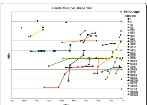
Hypothesis C The Pareto front of MFE versus MEA is comprised of a small number of macrostates, accompa-nied by essentially the same corona of microstates.
Akin to Pareto optimization, abstract shape analysis of RNA can give us an “interesting” set of alternative fold-ings [11]. They are characterized by the best-scoring structures having different abstract shapes. This idea being perfectly orthogonal to Pareto optimization, we give some attention to the question how abstract shapes and Pareto optima are related. Here we test the
Hypothesis D Abstract shape analysis and Pareto optimization produce about the same set of alternative “interesting” structures.
In the evaluation of hypotheses A–D, our test data for the MFE/MEA application consists of 331 RNA sequences of length 12–356 nucleotides, extracted from the full data set used in [33]. The data set is available with the supplementary material. For the Sankoff problem, we use sequences from two Rfam families. We use n1=19
PreQ1 RNA sequences (SSTRAND:RF_00522) and
n2=30 IRE RNA sequences (SSTRAND:RF_00037) extracted from the core data set of the Rfam database [34].
Algorithms implemented
We give a short sketch of how our algorithms are imple-mented. For each application, we can re-use grammars and algebras from the RNAshapes repository [35]. It is just the Pareto optimization which is new.
For the standard implementation, we tested the vari-ants pfisort, pfsort, pfsmooth, and pfnosort (cf. "Computing the Pareto front"). Fortunately, the standard implementa-tion can be mimicked in GAP-L without changing lan-guage or compilera. However, we can not evaluate the Pareto-eager implementation based on pflex with Bell-man’s GAP, as this would imply extension of GAP-L and modification of the sophisticated code generation in the Bellman’s GAP compiler.
In order to compare the Pareto-eager implementation to the others, we resorted to an implementation of ADP as a Haskell-embedded combinator language [23]. First, we added the variants pfisort, pfnosort, and pfsmooth for the standard implementation. Then, we designed a modi-fied set of combinators, corresponding to the outline in "Pareto-eager implementation". (For the expert: The key idea is to exploit monotonicity and compute the set {f(xi,yj)} of intermediate results represented as nested
lists in the form [[f(xi,yj)|j=1, ...]|i=1, ...]. For fixed xi,
the sublist [f(xi,yj)|j=1, ...] is sorted if the list [y1, , , ,] is.
This is ensured by structural induction and strict mono-tonicity of f on its second argument position). While this implementation is significantly slower than Bellman’s GAP code, it suffices to compare the Pareto-eager imple-mentation to its alternatives.
We use available building blocks for the independent optimizations: the RNA folding grammar OverDangle
(avoiding lonely base pairs) and the evaluation algebras
The size of the folding space X for a given sequence x
is independent of the optimization we perform. The Bell-man’s GAP compiler can automatically produce a count-ing algebra COUNT, that determines the size of the folding space. We run OverDangle(COUNT, x) on all our test data to get concrete folding space sizes, to be related to the sizes of their Pareto fronts.
The choice of k for a fair evaluation is not obvious. Selecting k=1 for MFE and MEA would be unfair, as
the Pareto front provides much deeper information. We considered using k=E(|X|,|x| =n), but the expected
size of the search space is not a good predictor, as |X| varies strongly with the sequence content of x. There-fore, we first run Pareto optimization on x, record the size of the Pareto front for this call, and then set k to this number when computing OverDangle(MFE(k), x) and
OverDangle(MEA(k), x).
Runtime and memory measurements This section and the next are devoted to our
Hypothesis A Pareto optimization in a realistic sce-nario is not more expensive than other approaches calcu-lating a similar amount of alternative answers.
We evaluate the performances of the Pareto front com-putation, using pfisort(X), pfsort(X), pfsmooth(X), and
pfnosort(X). Note that all compute the same Pareto front,
and hence have the same k in their asymptotics. For a fair comparison with two single-objective algorithms MFE and MEA, we use their versions MFE(k) and MEA(k), computing the k best structures under each objective. Here, k is set to the actual Pareto front size for the given input (which, of course, is only known because before we also compute the Pareto front with the other algorithms). All programs are compiled by the Bellman’s GAP com-piler using the same optimization options [29].
In Table 3 we show computation time and memory consumption, accumulated over all sequences and spe-cifically for the longest sequence. These are our main observations:
1. In terms of runtime, we find that the Pareto opti-mization performs not only better than the sum of the two independent optimizations, but also bet-ter than each of them individually. We attribute this to the fact that the Pareto algorithm adjusts itself to the size of the Pareto front, and this size tendsb to be smaller than k for small sub-problems. The search space itself, however, is exponentially larger than the Pareto front, and even on small sub-words it provides k near-optimals for MFE(k) and MEA(k) to spend computation on. This effect is strongest for
our longest sequence, where k=38 and the ratio of (MFE(k)+MEA(k))/pfnosort≈45.
2. The average case behaviour of pfnosort(X) is supe-rior to all the sorting implementations of pf. This is an unexpected and interesting observation. We attribute this to a positive randomization effect. Comparing a new element to the extremal points of the Pareto front, maximal in one but minimal in the other dimension, is unlikely to establish domination. This what always happens first with sorted interme-diate lists, and the element will walk along towards the middle of the list until it eventually is found to be dominated. In unsorted lists, a non-extremal ele-ment that dominates the new entry will, on average, be encountered earlier.
3. For evaluating the Pareto-eager strategy, we used the Haskell-embedded implementation. In the func-tional setting, pfisort required the least garbage col-lections and performed best. Somewhat unexpect-edly, the eager strategy was consistently a bit slower than pfisort and close to pfnosort, slower only by a factor varying between 1.0 and 1.2. It was faster than pfsmooth, in turn by a factor between 1.1 and 1.5. 4. Memory consumption of Pareto optimization is
consistent over different implementations of pf. It is higher than either MFE(k) or MEA(k) alone, but clearly less than the sum of MFE(k) and MEA(k). This is better than expected, because after all, it solves both problems simultaneously.
Note that the above values are measurements of con-stant factors, and averaged over many runs. So, pfnosort is not always faster than pfsmooth. In fact, we have seen cases where pfnosort is faster than pfsmooth for pf>A,>B, but slower for pf>A,<B (where in the latter case, we switch from maximization to minimization in algebra B).
Table 3 Runtimes and memory requirements for MFE(k),
MEA(k) (where k is the empirical Pareto front size for a given input), and their Pareto product (MFE∗ParMEA),
accumulated over 331 sequences (left) and for the longest sequence (n=356,k=38, right)
The computations were performed by using Bellman’s GAP.
Algebra Time (min) Memory (GB) Time (min) Memory (GB)
MFE(k) alone 71 163.68 5 1.16
MEA(k) alone 61 153.51 5 1.05
MFE(k) + MEA(k)132 (+) 163.68 (max) 10 1.16 (max) (MFE∗ParMEA)
pfnosort 8 197.28 0.22 1.28
pfsmooth 9.5 192.79 0.5 1.28
pfsort 18 271.21 1 1.28
Pareto front size
The size of the Pareto front is of critical practical impor-tance. Pareto front sizes in the hundreds, even for sequences of moderate length, would be prohibitive. The number of solutions in the Pareto front depends on the data. Not only on the sequence length and the size of the search space in our RNA folding scenario, but also on the actual structures found. For example, if there is a very prominent structure in the folding space, it will dominate many other solutions in both objectives, and the Pareto front will be small. On the other hand, in one case we observed a Pareto front of size ≈ |x| with the program of Schnattinger et al. on a Sankoff-style algorithm, an effect we will study in detail below.
Figure 1 shows our measurements. We observe the following:
• Pareto front sizes are quite moderate, ranging round 10 for n=100, 15 for n=200, up to 45 for n=274 . Specifically, our longest sequence (n=356) has a Pareto front of size 38.
• Variance is high (as expected), and because of the strong variation, we did not fit a line through our measurement points. However, they are all domi-nated by the expected size of the Pareto front (red line).
• We did not smooth the graph for H(|X|), such that it also demonstrates the variance in the search space sizes; just read the y-axis as a logarithmic scale for eH(|X|). The roughly linear behavior conforms with the theoretical analysis.
The moderate sizes of Pareto fronts in our applications also imply that no benefit is to be expected from using quad-tree data structures in place of our sorted list rep-resentation. According to measurements in [36], popula-tion sizes in the thousands are required to make the more sophisticated data structure pay off.
Summing up our empirical data, we state that Hypoth-esis A has been confirmed in general, which does not rule out that there are problematic cases. One of these is dis-cussed next.
Anti‑correlation and real worst case behaviour
Two scoring functions are correlated to the extent by which they rank the candidates of the search space in the same order. Perfect correlation or anti-correlation would render a combined application of both objectives meaningless. Perfect positive correlation implies that an optimal candidate under >A is also optimal under >B, so nothing is to be gained from optimizing with respect to >B. Perfect anti-correlation means that the optimal candidates under >B are the worst candidates under >A.
Hence, they can also be obtained as the optimal candi-dates optimizing under <A alone. In interesting scenar-ios, we can expect the two scoring schemes to correlate in some of the local scoring functions, and anti-correlate in others.
Anti-correlation can make the worst case real, where the size of the Pareto front does not follow the Har-monic law, but is linear the size of the interval of score values actually occurring (cf. Observation 3). There is a minor flaw in the objective function used in [20],
0 50 100 150 200 250 300 350
02
04
06
08
0
100
120
Pareto front size in function of the sequence size.
Sequence size.
Pa
reto front si
ze
.
Expected Pareto font size Pareto font size
0 50 100 150 200 250 300 350
05
10
15
20
Number of Shape in function of the sequence size.
Sequence size.
Number of shapes
.
Number of RNAshape
a
b
Figure 1 a Empirical Pareto front size of OverDangle(MFE∗ParMEA,x)