Spotting The Wisdom In The Crowds

(1)

Imperial College London

Department of Computing

MSci Joint Mathematics and Computer Science Individual Project Final Report

Spotting The Wisdom In

The Crowds

Liam Williams

ldw08@ic.ac.uk

Supervisor: Second Marker:

Dr. William Knottenbelt Dr. Giuliano Casale

(2)

Abstract

The growing popularity of websites on which hundreds of “tipsters” provide sporting tips has resulted in a large influx of sports betting advice in the public domain. But how do we know which of these tips are “reliable” and which should not be trusted? How do we spot the wisdom which may be hiding in the crowds?

The aim of this project is to investigate to what extent it is possible to extract such reliable advice from a large group of tipsters by observing the historical betting patterns of the population. Previous research into the performance of sporting tipsters has been limited to much smaller population sizes, for example those with regular newspaper columns.

We consider a simulated world, which is used to investigate a variety of potential scenarios regarding the behaviour of the tipsters in the population. In this controlled environment, we are able to develop and validate methods for detecting and extracting the wisdom. We then look at a particular real world tipping website which considers only the tennis win market. Apply-ing the techniques developed whilst investigatApply-ing the simulated world, we find that although high precision rates are achievable, it is much more of a challenge to obtain a significant positive return on investment.

(3)

Acknowledgements

I would like to thank my supervisor Dr. William Knottenbelt for his support and guidance over the course of the project, as well as his level-headedness on the numerous occasions I exclaimed “I’ve cracked it, we’re rich!” only to find out that something was amiss.

Thanks also go to the staff at Active Capital Management, whose initial ideas and suggestions helped to give the project the kick start it needed.

Finally I would like to thank my friends and especially my family for their patience and support these past four years and without whom I would not be where I am today.

(4)

3.1.3 Math.NET Numerics . . . 27 3.1.4 ALGLIB . . . 27 3.1.5 Emgu CV . . . 27 3.1.6 NHibernate . . . 27 3.1.7 SQLite . . . 27 3.1.8 Html Agility Pack . . . 28 3.1.9 NUnit . . . 28 3.2 Persistence . . . 28 3.2.1 Database Design . . . 28 3.2.2 Persistence Layer . . . 29 3.2.3 Storage Mechanism . . . 30 3.3 Scrapers . . . 30 3.3.1 TennisInsight . . . 30 3.4 Simulated World . . . 31 3.4.1 System Overview . . . 31 3.4.2 XML Specification . . . 33 3.5 Analysis . . . 33 3.5.1 Classifiers . . . 33

(6)

3.5.2 Grid Search . . . 33 3.5.3 Cross Validation . . . 34 3.5.4 Experiments . . . 34 3.6 Testing . . . 34 3.6.1 Unit Testing . . . 34 3.6.2 Acceptance Testing . . . 35

4 Simulated World Investigation 36 4.1 The Need For a Baseline Population . . . 36

4.1.1 Data Representation . . . 37

4.1.2 Filtering . . . 39

4.2 Experiments . . . 41

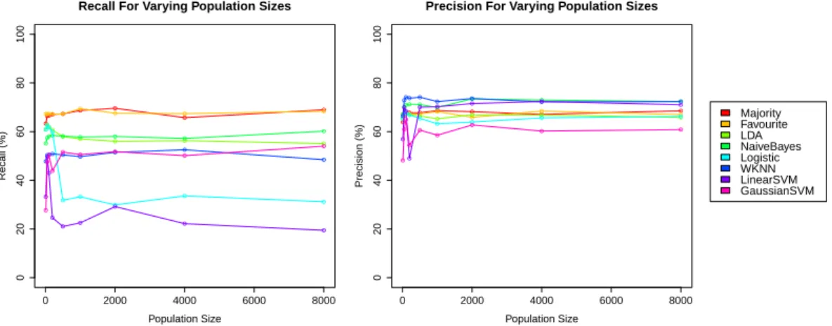
4.2.1 Population Size . . . 41

4.2.2 Proportion of Smart Tipsters . . . 43

4.2.3 Edge of Smart Tipsters . . . 44

4.2.4 Copycat Tipsters . . . 45 4.2.5 Tipping Frequency . . . 45 4.2.6 Discrete Bets . . . 46 4.2.7 Specialist Tipsters . . . 46 4.2.8 Too Smart? . . . 48 4.3 Summary . . . 49

5 Real World Investigation 50 5.1 Overview of Data . . . 50

5.1.1 Monthly Site Overview . . . 50

5.1.2 Tipster Behaviour . . . 51

5.1.3 Random Behaviour? . . . 52

5.1.4 Profitable Behaviour? . . . 53

5.1.5 Population Significance . . . 53

5.1.6 Better Than Favourite Selection? . . . 54

5.1.7 Summary . . . 56

5.2 Analysis . . . 57

5.2.1 Cleaning The Data . . . 57

5.2.2 Look Back Periods . . . 57

5.2.3 Final Test Data . . . 58

5.2.4 Bahamas Or Bust! . . . 59

5.3 One Last Try . . . 63

5.3.1 Modified Weighted K Nearest Neighbour . . . 63

5.3.2 Performance . . . 64

(7)

5.4 What About The Tipsters? . . . 66

6 Discussion 68 6.1 Summary Of Findings . . . 68

6.2 Future Work . . . 69

6.2.1 Alternative Approaches . . . 69

6.2.2 Shorter Retraining Intervals . . . 69

6.2.3 Markets With Several Outcomes . . . 69

6.2.4 We Need More Data! . . . 70

6.2.5 Bookmakers As Tipsters . . . 70

6.2.6 A New Tipping Website . . . 71

A Odds 72 A.1 Representation . . . 72

A.1.1 Fractional . . . 72

A.1.2 Decimal . . . 72

A.1.3 Conversion . . . 72

A.1.4 Implied Probability . . . 73

A.2 Bookmakers . . . 73

A.2.1 Over-round . . . 73

A.2.2 Normalised Implied Probabilities . . . 73

B Details 74 B.1 Naive Bayes Classifier . . . 74

B.2 Linear Discriminant Analysis . . . 75

B.2.1 Details On Method . . . 75

B.2.2 Classification . . . 75

B.2.3 Feature Selection . . . 76

B.3 Expected Mean Profit Of The Random Strategy . . . 76

(8)

List of Figures

2.1 Smart Probability Adjustment . . . 10

2.2 Comparison of PCA and LDA . . . 15

2.3 Naive Bayes Classifier . . . 16

2.4 Linear Support Vector Machine . . . 19

2.5 K Nearest Neighbour Classification . . . 20

2.6 Non-linear Support Vector Machine . . . 20

2.7 Auxiliary Cross Validation For Choosing Classifier Parameters . . . 23

3.1 Relationships Between Main Data Entities . . . 29

3.2 TennisInsight Tip History Page Example . . . 31

3.3 Simulation System Overview . . . 32

3.4 Selection To Matrix Classifiers . . . 34

4.1 Data Representation Precision . . . 37

4.2 Data Representation Recall . . . 38

4.3 Filtered Baseline Data Performance . . . 40

4.4 Varying Population Sizes (Direct Approach) . . . 42

4.5 Varying Population Sizes (LDA Compressed) . . . 42

4.6 Varying Population Sizes (Significant Strike Compressed) . . . 43

4.7 Varying Proportions of Smart Tipsters . . . 43

4.8 Varying Edge of Smart Tipsters . . . 44

4.9 Varying Number Of Original Opinions . . . 45

4.10 Varying Tipping Frequency . . . 46

4.11 Varying Discreteness . . . 46

4.12 Varying Number Of Expert Groups (Unaware) . . . 47

4.13 Varying Number Of Expert Groups (Aware) . . . 47

4.14 Ignoring The Market . . . 48

5.1 TennisInsight Monthly Overview . . . 51

5.2 TennisInsight Population Activity . . . 52

5.3 TennisInsight Sample Returns . . . 53

(9)

5.5 TennisInsight Population Performance . . . 54

5.6 TennisInsight KS Tests . . . 55

5.7 TennisInsight KS Test Returns . . . 56

5.8 TennisInsight Data Split . . . 57

5.9 TennisInsight Look Back Periods . . . 58

5.10 TennisInsight Over-Round Distribution) . . . 60

5.11 TennisInsight Flat Profit Streams (Stake Representation) . . . 60

5.12 TennisInsight Flat Profit Streams (Odds Representation) . . . 61

5.13 TennisInsight Kelly Profit Streams (Stake Representation) . . . 62

5.14 TennisInsight Kelly Profit Streams (Odds Representation) . . . 63

5.15 MKNN Distance Weighting . . . 64

5.16 TennisInsight MKNN Profit Stream . . . 65

5.17 Odds Taken By MKNN . . . 65

5.18 Crowd Sourcing A Stake Strategy . . . 66

(10)

List of Tables

2.1 Classification Cases . . . 21

2.2 Summary Of Classifier Hyper Parameters . . . 22

4.1 Baseline Flat ROI Under Odds/Stake Representations . . . 38

5.1 TennisInsight Final Recall and Precision (Stake Representation) . . . 58

(11)

1

Introduction

In this chapter, we will look at the problems considered in the project and the approach taken to tackling them. Section 1.1 gives an overview of what the scope of the project is and why it is worth undertaking, as well as the challenges we face in arriving at a solution. Section 1.2 lists the main contributions of the project and finally, Section 1.3 provides a brief summary of the report organisation.

1.1 Motivation

Before the advent of the Internet, perhaps the most common public source for sporting tips was that offered by professional tipsters published in newspapers. In recent years, websites on which “expert” tipsters provide public tips have grown in popularity, see

e.g. TennisInsight1 _{and OLBG}2_{. As a result of this, there is a much greater volume of}

tips in the public domain than there has been in the past.

The question remains: is it possible to tell which of these tips are “reliable” and which are not; is it possible to spot the wisdom which may be hiding in the crowds?

The main aim of this project is to perform an analysis of the sporting tips given on such tipping websites to investigate how well tipsters perform when considered individually and also as a group. Additionally, we develop a “meta-tipster” which aims to identify correlations in tipsters betting patterns which are then used to provide a classification for future tips.

We begin by constructing a simulated world, where some of the desirable properties of the real-world data are artificially made present, for example giving a subset of tipsters a consistent edge in predicting events. This is done to show that, if such phenomena were to occur, it would be possible to pick up on this information by considering the betting patterns of the tipsters.

Ultimately, any new tip offered by the tipsters is to be classified according to whether the prediction is expected to become a reality or not. We consider several approaches

1_{http://www.tennisinsight.com/} 2_{http://www.olbg.com/}

(12)

1.2. Contributions Chapter 1. Introduction

to making this binary classification, using techniques from the areas of statistics and machine learning.

We consider several different configurations of the simulated world and evaluate the performance of the different approaches to classification by the meta-tipster to identify which kind of classifier is most appropriate given the underlying structure of the data. Performance is evaluated against a naive majority voting approach and selection using the bookmakers implied odds to select the most probable outcome of an event according to the bookmakers, or “favourite” selection. Outperforming favourite selection may indicate that, collectively, the tipsters have private information that the public odds information alone does not encompass.

The performance of the meta-tipster is then evaluated using historical data collected from publicly available tip histories on TennisInsight. The TennisInsight data set comprises of approximately half a million tips made between May 2008 and December 2011 by approximately two thousand tipsters.

The period of time over which to consider historical data for training a classifier is also considered; tipster’s models are subject to change in a real world situation, so looking at the entire past year’s data may not be a good idea if tipsters tend to adapt their models more frequently than this. In practise, one might expect to have to periodically re-train classifiers to keep up with recent trends. Another point is that not all tipsters will stay active on a site indefinitely; there is no point considering tipsters who are no longer providing new tips.

Finally we examine the potential return on investment (ROI) that could have been achieved by following the advice of each of the classifiers over a period of time spanning 2010 and 2011. Several stake sizing strategies are considered, including a Kelly betting strategy, flat stake and crowd sourcing the amount to stake.

1.2 Contributions

The main contributions of the project are:

• A simulated world which can be used to generate different populations of tipsters

which tip events with markets that have a finite number of possible outcomes.

• Using the simulated world to examine the effect deviations from a baseline

popu-lation have on the predictive ability of the various classifiers considered.

• An investigation into the real-world TennisInsight data set, including making use

of historical data to evaluate the performance of the meta-tipster and leading on to a final evaluation which looks at the potential return on investment which could have been achieved, had the advice of the meta-tipster been followed.

1.3 Report Organization

(13)

1.3. Report Organization Chapter 1. Introduction

Chapter 2 providesbackgroundinformation on the tools and techniques used, as well

as considering existingrelated workin the context of the project.

Chapter 3 goes into some of the details of the implementation, including data

col-lection and storage, the simulated world and use of existing technology to form the various classifiers.

Chapter 4 investigates thesimulated world, which provides a controlled environment

for finding out which kinds of situation make it possible to spot the wisdom. Starting with a baseline population, which is used as a frame of reference when evaluating the performance of the meta-tipster, we make a number of changes to the baseline population and evaluate their effect on the predictive performance of the meta-tipster.

Chapter 5 investigates the real world data obtained from TennisInsight, first

at-tempting to get an idea of the typical behaviour of the population of tipsters. We then apply the meta-tipster approach to the real world data, considering the

effect of different “look-back” period lengths and then performing a final

eval-uation of both the predictive performance of the meta-tipster and the potential

return on investment that could have been achieved.

Chapter 6 provides a discussion of the main findings of the project, drawing

com-parisons between the simulated populations considered and the real world data.

(14)

2

Background

This chapter contains the relevant background information that was considered to arrive at a solution. Section 2.1 discusses previous related work in the area of forecasting sporting events and how this project will cover new ground. Section 2.2 provides a brief reference for some terminology which will be used throughout the report. In Section 2.3, several possible problem representations considered, as well as appropriate normalisation methods. Section 2.4 explains the approach taken in constructing the simulated world. Section 2.5 gives background information on the tipping websites which were considered as sources of data. Section 2.6 discusses the approaches for data storage that were considered. Section 2.7 considers different ways of achieving dimensionality reduction. Section 2.8 explores several different types of binary classifier. Finally, a number of different stake sizing strategies are considered in Section 2.9.

2.1 Related Work

Previous work in assessing the performance of experts in the context of forecasting sport-ing events was found to be limited. The general consensus for judgemental forecastsport-ing appears to be that “in nearly all cases where the data can be quantified, the predictions of the [statistical] models are superior to those of the expert”[23], apart from the case

when “broken-leg cues”1 _{are available to the expert.}

Forrest and Simmons[15] examined the performance of newspaper football tipsters when forecasting the results of English league matches; their analysis was limited to just three tipsters. The tipsters in this case were found, individually, to perform poorly; even the simple strategy of always picking the home team (which has been shown to have an advantage over the away team previously[8]) was found to yield a better strike rate, however all of them demonstrated some underlying knowledge of football above just picking results at random.

Considering each tipster’s forecasts individually against a simple statistical model con-structed using public information, only one of the three tipsters was found to be making 1_{A broken-leg cue refers to an unusual important piece of information whose presence would} dramat-ically alter judgement compared to a model of that judgement[38]

(15)

2.1. Related Work Chapter 2. Background

use of some form of private or semi-public information. However, when combining the tipsters predictions and taking a consensus (i.e. when two or more tipsters agreed), the

conclusion was that the consensus forecast did add some explanatory power above just

using the public variables.

In later work by Forrest et al[14], the performance of the odds-setters (i.e. bookmakers) as forecasters is considered against a benchmark statistical model, concluding thatall of the British bookmakers considered appear to individually be privy to, and make effective use of, information not included in the benchmark model.

Andersson et al[2, 3] look at the performance and confidence of experts and laypeople in forecasting outcomes of the football World Cup, finding that both groups surveyed had similar levels of performance (which was better than chance) in predicting match outcomes. Unfortunately, a simple rule following world rankings was found to outperform the majority of participants. In predicting more complex outcomes such as full time scores and ball possession, however, the experts were found to outperform the na¨ıve participants. In all cases, the experts were found to be significantly more confident about their forecasts than the laypeople.

Player name recognition has also been considered as a method in which lay predictions can be made. Pachur and Biele[27] find that a recognition heuristic agreed with lay forecasts for the European Football Championships 2004 in 90% of cases, suggesting that laypeople do tend to use player name recognition to make their predictions. The heuristic was found to perform significantly better than chance, but was outperformed by a model based on direct indicators of team strength.

Scheibehenne and Broder[32] look into player name recognition by laypeople for pre-dicting the 2005 Wimbledon Gentlemen’s tennis competition. Predictions based on this were found to perform at least as well as predictions based on official rankings, however online betting odds led to more accurate forecasts.

Bruno Deschamps and Olivier Gergaud[12] investigate the originality (i.e. excessive variation from the public information given their private information) of 35 professional French horse racing tipsters, finding that the tipsters were indeed more original than not. However, it is found that forecasts would have been more accurate if the tipsters had deviated less from the public information.

Something which does not appear to have been investigated previously is how the inter-actions between tipster’s betting patterns may be a good indicator of the true outcome of an event. Consensus voting is a simple example of these kind of interactions, but it is suspected that there is more underlying structure due to the conflicting models which tipsters use to make their predictions, which is a further motivation for this investigation. To illustrate, each tipster can be assumed to have a model which they use to choose which tips to bet on. This model may be backed by an actual statistical model or could be something less tangible, such as player name recognition or some other heuristic method.

Some of these models may completely dominate others, i.e. model A dominates model B if A predicts correctly in all of the cases which B does, as well as in additional cases where B does not predict correctly.

(16)

2.2. Terminology Chapter 2. Background

Certain models may be better at predicting different kinds of cases; one model may be good at predicting the “usual” continuous cases, but may completely fail when something unexpected happens, take the literal case of a player breaking their leg. Another model, from a tipster who pays more attention to such discontinuities would be the advice to

follow in this case, however this advice maynot be the popular opinion of all tipsters.

2.2 Terminology

Site

A tipping website (e.g. TennisInsight) where tipsters make tips. Sport

A sport can be either a literal sport (e.g tennis) or a contrived sport (e.g. OLBG offers betting on “specials” such as the outcome of awards such as the Golden Globes).

Match

An instance of a sporting event (e.g. a single football match). Market

A market for a particular sport consisting of several possible outcomes (referred to as “runners”) which depend on the outcome of a particular match (e.g. a tennis match has a win market and a set betting market).

Runner

A possible outcome of a market. (e.g. for the tennis win market, the runners are the competing players and for the football full time result market, the runners are the competing teams and the draw outcome).

Tipster

An “expert” who makes tips on a site (e.g. a member of TennisInsight). Tip

A selection of a particular runner for a certain market and match which a tipster is recommending. Includes the stake (i.e. amount of money bet) and odds taken by the tipster (odds are offered by bookmakers that are independent of the site the tip is placed on).

Selection

A selection refers to the choice of a single runner for a particular market and match. The term is used since different tipsters can make tips for the same selection.

2.3 Problem Representation

For each tip offered by a tipster for a particular match, market and runner (referred to as a selection), there is data available on stake size and odds taken by each tipster. This can be represented as the feature vector:

s1 o1 . . . sn on

(17)

2.3. Problem Representation Chapter 2. Background

wherenis the number of tipsters, oj represents the odds taken andsj the stake laid out by tipster j.

As an example, suppose we have two tipsters, Alice and Bob, who have each placed a stake of 10 units on a particular player to win a tennis match, however Alice has taken odds of 1.2 and Bob has taken odds of 1.1. Additionally a third tipster, Charlie, is also considered, but did not happen to place any bets at all for this particular match. Then the corresponding feature vector is:

Alice z }| { Bob z }| { Charlie z}|{ 10 1.2 10 1.1 0 0

For a collection ofm selections, the corresponding feature vector for each selection can

be written as the rows of the matrix:    s11 o11 . . . s1n o1n .. . ... ... ... sm1 om1 . . . smn omn   

Here,oij represents the odds taken and sij the stake laid out by tipsterj for selectioni (with oij =sij = 0 if the tipster did not tip this selection).

Each selection has a class associated with it, corresponding to whether the result of the associated match resulted in this selection being the correct result for the associated market or not.

It is possible that the number of tipsters to be considered will be large, perhaps thou-sands, which means a large number of dimensions for the feature vectors.

This potentially high dimensional space is problematic. This is due to both practical reasons (e.g. computation begins to become intractable) and also because, since it is

possible thatmn, such that the amount of available data will be sparse, the so-called

“curse of dimensionality”. Possible ways to reduce the dimensionality of the problem are discussed in Section 2.7.

2.3.1 Alternatives

Clearly, this is not the only way to formulate the problem and several variations of this model will be considered.

The stake size and odds taken are considered important since it seems likely that tipsters will “bet their beliefs” and size their bets according to the edge that they consider to have over the odds offered by the bookmaker.

It may not only be important to consider the details of who did or did not support a

particular selection, but also, in the case that a particular tipster did not support the

selection, if they instead supported a different selection or perhaps supported none at all.

Note that tipsters are assumed to only be “allowed” to support one selection per match and market (something which is enforced on TennisInsight and OLBG).

(18)

2.3. Problem Representation Chapter 2. Background

In light of this, the original feature vector can be extended: s1 o1 s∗1 o∗1 . . . sn on s∗n o∗n

where the additional variabless∗_i and o∗_i represent the stake laid out and odds taken by the tipster if they supported a different runner for the same match and market as the selection in question, withs∗

i =o∗i = 0 if the tipster did not support a different runner. So ifsi=oi =s∗i =o∗i = 0 for a particular tipster, this represents that they did not have a tip for this match and market. Representations which include this type of information will be referred to as “and not” versions.

This representation makes more sense if we are considering markets with more than two possible outcomes. Suppose there were three possible outcomes for the market that Alice and Bob had bet on, then the corresponding feature vectors for all three selections would be: Alice z }| { Bob z }| { Charlie z }| {   10 1.2 0 0 10 1.1 0 0 0 0 0 0 0 0 10 1.2 0 0 10 1.1 0 0 0 0 0 0 10 1.2 0 0 10 1.1 0 0 0 0  

The benefit of this is that there is now a distinction between not betting on anything at all (corresponding to all zeros for that tipster as in the case of Charlie) and betting on

something which wasnot this (see e.g. the second row for Alice).

Another representation is to simply have a binary indicator variable, corresponding to whether or not the tipster supported the selection, instead of the stake size and odds variables; the feature vector is just:

t1 t∗1 . . . tn t∗n

whereti= 1 if the tipster did support the selection andt∗i = 1 if the tipster supported a different selection. Ifti =t∗i = 0, this again represents that they did not have a tip for this match and market.

A benefit of all of the representations considered is that they are all able to cope with markets containing any number of outcomes and even a variable number of outcomes (which could be useful in representing, say, horse racing markets which have a variable number of runners per race).

2.3.2 Normalisation

Clearly, each of the features are not all the in the same units (e.g odds, stake size) and so appropriate normalisation of each feature can be carried out as a pre-processing step. One way to do this is to mean centre and scale to unit variance by dividing by the empirical mean and standard deviation. A problem with this is that, since the data will

be sparse (i.e. it is unreasonable to expect that all of the tipsters will provide a tip

for every match), this transformation will destroy the sparsity since each feature will typically have a different normalisation constant.

(19)

2.4. Simulated World Chapter 2. Background

Another way to handle this in the case of stake sizes is to represent the stake size as a percentage of the previously observed maximum stake size for the tipster in question, which does preserve sparsity and normalises stake size to the range [0,1].

Odds can also can be normalised to the range [0,1] by representing them using the

corresponding implied probabilities (see Appendix A.1.4).

As an example, returning to the basic stake and odds representation with the Alice and Bob example, the feature vector

Alice z }| { Bob z }| { 10 1.2 10 1.1 might be normalised to Alice z }| { Bob z }| { 10 100 1 1.2 10 10 1 1.1

if the maximum stake size for Alice were 100 units and the maximum stake size for Bob were 10 units.

2.4 Simulated World

To construct the simulated world, we need three main components: the matches, the odds setter and the population of tipsters who have the opportunity to place bets on the markets associated with these matches according to the odds set by the odds setter.

2.4.1 Generating “True” Probabilities

Given a match which has a market with nrunners, the distribution of winning runners

can be said to be categorically distributed, where the probability of runner xi winning

ispi, constrained by:

n X

i=1

pi = 1

The “true” probabilitiespifor each of thenrunners are generated by samplingµi ∈[0,1] from the uniform distribution on [0,1], and then constructing the corresponding pi as:

pi= µi Pn

j=1µj

For example, with n = 2, if µ1, µ2 are randomly selected as µ1 = 0.4, µ2 = 0.8 then

p1 = ₀_.₄₊₀0.4_.₈ ≈0.33 andp2 = ₀_.₄₊₀0.8_.₈ ≈0.66.

2.4.2 Estimation Strategies

A tipster has estimates ˆpi (summing to 1) which they hope correspond to the true pi

(i.e. _|pˆi−pi| ∈[0,1] is small for all i). The process of finding these ˆpi is referred to as an estimation strategy.

(20)

Random

A random estimation strategy forms estimates ˆpi using the same method in which the

“true” probabilities were distributed, so that ˆpi can vary completely from the truepi.

Smart

Tipsters can be artificially instilled with wisdom such that their estimates do not differ a great deal from the true probabilities of each runner in the market.

To introduce this error, each true probability pi is adjusted by adding a random value

ri sampled from the uniform distribution on [−rpi, r(1−pi)] for a fixed r ∈[0,1]. The resulting adjusted probabilities will not sum to 1, so the estimates ˆpi are taken as:

ˆ pi=

pi+ri Pn

j=1(pj+rj)

Nowrcan be used to change how reliable the estimates are; increasing rallows the

esti-mates to vary more from the true probabilities, where atr = 1 each of the probabilities

have a chance of being adjusted to estimates wildly different from the true probabilities, whilst atr= 0, ˆpi=pi and the estimations are perfect. This is illustrated in Figure 2.1.

1

0 pi

rpi r(1−pi)

Figure 2.1: Smart Probability Adjustment

2.4.3 Specialist Tipsters

To model the idea that tipsters may have a certain type of match that they are a “specialist” on, sets of tipsters,Ti, are assigned a subset of all matches that they will be

“smart” on, Mi, which is disjoint from all other sets of matches assigned to the other

sets of tipsters (i.e. Mi∩Mj =∅ ∀i6=j).

For all matches m /∈Mi, which the tipsters Ti are not specialists on, the tipsters may either decide to simply behave randomly, or alternatively, if they are aware that they are not a specialist on a particular match, may simply abstain from tipping that match.

Variations of this can be considered, for example where the sets of assigned matchesMi

are no longer disjoint and so there is some overlap in the matches which the groups of tipsters are specialists for.

2.4.4 Copycat Tipsters

Some groups of tipsters will follow the advice of a “pack leader” and copy the leader’s actions, regardless of whether the leader’s decision happens to be a good one or a bad one. This can be used to model the idea that a popular opinion may not always be the

(21)

correct one. Having a large number of copycat tipsters may have a significant influence on the consensus of the population.

2.4.5 Odds Offered

Tipsters are offered odds by an odds-setter, who uses a smart estimation strategy with

(typically) small r to set these odds. The odds set are taken as the reciprocal of the

probability estimates (the estimates correspond to the implied probabilities which can be calculated from offered odds and may include over-round in a real world situation,

see Appendix A.2.2), denoted ˜pi. Here we assume no over-round is introduced.

2.4.6 Selection Strategies

Given that a simulated tipster has a set of estimates ˆpi for each runnerxi, they can now use these to decide which runner to select, if any.

Most Edge

The tipster can calculate the discrepancydi between their estimate ˆpi and the implied probability of the odds offered by the odds-setter ˜pi:

di = ˆpi−p˜i∈[−1,1]

Positive discrepancy indicates that the tipster’s estimate of the runner winning is greater than the odds-setter’s estimate; in other words, the tipster is more confident than the odds-setter that this runner will win. A positive discrepancy of 1 would indicate that the tipster has estimated that this runner is certain to win, whilst the odds-setter has estimated that they are certain to lose.

Similarly, negative discrepancy indicates that the tipster isless confident than the

odds-setter that this runner will win. A negative discrepancy of ₋1 would indicate that

the tipster has estimated that this runner is certain to lose, whilst the odds-setter has estimated that they are certain to win.

It is therefore in the best interests of the tipster to only make a selection when there exists a runner xi with di > dmin, where dmin ∈ (0,1] is the minimum positive edge the tipster is prepared to place a bet on. When such a runner does exist, if there are multiple such runners, the one with the greatest discrepancy value is chosen.

Ignore The Market

Alternatively, a tipster may decide to take no notice of the implied probability of the odds offered and instead simply choose the runner with the largest predicted probability of winning ˆpi. In this case we will takedi = ˆpi for simplicity.

(22)

2.5. Real World Data Chapter 2. Background

2.4.7 Stake Sizing Strategies

Given that a tipster has selected a runner xi with corresponding discrepancydi > dmin, they must now decide how much to stake on this runner. The process of deciding on a stake size is referred to as a stake sizing strategy.

Fixed

The tipster always bets the same amount, say B, regardless of the edge they consider

they have.

Scaled

The tipster bets an amount f(di)·Bmax wheref is monotonically increasing on [0,1]. For example,f(di) =dλi could be used for some fixed λ≥1.

When λ= 1 we will refer to this as a “proportional” stake sizing strategy.

2.4.8 Experiments

By combining tipsters with different underlying estimation, selection and stake sizing strategies, different experiments can be set up to simulate data from different populations of tipsters. Chapter 4 goes on to investigate the effects changes in the population have on being able to spot the wisdom in the crowds.

2.5 Real World Data

Two tipping websites were considered as a source of real world data for the project, TennisInsight and OLBG. Ultimately only TennisInsight data was used for analysis, due to problems in collecting data from OLBG, discussed in Section 3.3.

2.5.1 TennisInsight

TennisInsight allows tipsters to tip on the win market for professional tennis matches using an unlimited amount of virtual money. Odds are offered by tracking the best odds offered by various bookmakers.

The site provides specialist information in the form of variety of statistics for the ten-nis players (i.e. indicators of their past performance) which is only accessible to paid subscribers.

Current tips made by tipsters are also only visible by paid subscribers, with the exception of the next upcoming match. Tip histories from 2008 to the present are publicly available for all non-current matches.

(23)

2.6. Data Storage Chapter 2. Background

Leader boards for tipsters recent performance exist (e.g. ROI, strike rate, amount earned), which could be seen as a source of motivation for the tipsters.

The investigation into the TennisInsight data can be found in Chapter 5.

2.5.2 OLBG

OLBG allows tipsters to tip on a variety of markets for a number of different sports, such as tennis, football, rugby, darts, and horse racing. Like TennisInsight, odds are offered by tracking the best odds offered by various bookmakers. Tipsters have a limited amount of virtual money, which is supplemented periodically to represent income. There is no form of paid subscription. Tip histories are publicly available for the past 45 days only. No form of specialist information is given for the various sports.

The site offers “free” bets which are sponsored by bookmakers and cash prizes in monthly competitions as incentives for tipsters to perform well.

2.6 Data Storage

2.6.1 Relational Databases

A relational database can be used to store data as a “set of formally-described tables from which data can be accessed or reassembled in many different ways without having to reorganize the database tables”2 _.

In the context of the data that will be simulated or collected, the relational database is an appropriate storage solution since the data will be analysed in a variety of different (and potentially unforeseen) ways, which will require querying the data in different ways. If a flat file approach to storing the data were taken, it would be more difficult to achieve this, whereas a database solution keeps things flexible.

2.6.2 Serialization

Serialization in the context of object oriented programming languages refers to the pro-cess of converting an in-memory object to a serialized form which can be persisted to a file (or even to a database) and read back into memory at a later date. This may be a suitable technique for caching transformed data which takes a significant amount of time to compute. For example this could be useful for persisting trained classifiers.

2.7 Dimensionality Reduction

It is possible that we will be dealing with datasets consisting of thousands of tipsters, corresponding to a very high dimensional feature space, which could be problematic

(24)

2.7. Dimensionality Reduction Chapter 2. Background

both in terms of computational feasibility and efficiency of the classifiers. As such, we consider several ways to reduce the dimensionality of the problem.

2.7.1 General Techniques

If there is not a lot of data for a particular feature, it may makes sense to exclude that feature. In this context, this would mean excluding tips by tipsters who have made less than some threshold number of tips.

2.7.2 Principal Component Analysis

Principal Component Analysis (PCA)[1, 20, 28] is a technique used for finding patterns in high dimensional data.

An orthogonal transformation is used to transform data to a new coordinate system which better explains the variance in the data, such that a small number of the basis vectors (or principal components) in the new coordinate system may explain the majority of the variance in the data. By projecting data onto the space spanned by a subset of the basis vectors, the dimensionality of the data can be reduced.

PCA can be a useful technique for visualising high dimensional data, by projecting data using just the first two or three principal components, but this should not be taken as an end in itself[41], but more as a guide for further investigation.

A strong assumption made by PCA is that large variances have important structure[34] which is something which may be incorrect in practice, depending on the particular problem (see Figure 2.2).

2.7.3 Linear Discriminant Analysis

Linear Discriminant Analysis (LDA)[13, 16] is, similar to PCA, used to find patterns in high dimensional data.

Unlike PCA, the goal of LDA is to find a new coordinate system which best explains how to discriminate between two or more classes, where each data point is associated with a class. This can be useful when the discriminatory information is not contained in the variance of the data, but in the mean (see Figure 2.2).

A fundamental assumption of LDA is that the independent variables are normally dis-tributed, which may be unreasonable to assume in this context, however it is still a technique worth investigating since the underlying structure of the data is not yet known. It is important to note that, since we are dealing with a two class problem, the number of non-zero eigenvectors will be just one; we will be reducing the dimensionality of the data down to just one dimension, which may have limited applicability.

A more practical way to use LDA as a dimensionality reduction technique is considered, where the magnitude of the factor loadings is used to rank the importance of each

(25)

2.8. Binary Classification Chapter 2. Background

dimensionality we wish to reduce to.

Details of LDA can be found in Appendix B.2.

Figure 2.2: Comparison of PCA and LDA3

2.8 Binary Classification

The aim of a binary classifier in this context is to take a feature vector (see Section 2.3) and determine which class it belongs to. In other words, given a particular selection, the classifier will predict whether it expects the selection to become a reality (i.e. to win) or not by assigning it to one of these two classes.

2.8.1 Simple Majority Voting

A simple majority voting classifier counts the number of tipsters who supported a se-lection and compares this to the count of tipsters for all other sese-lections for the same match and market. The classification is then based on whether the selection in question has the support of the majority of tipsters or not.

2.8.2 Favourite Strategy

Another simple strategy which only makes use of the public odds information is to simply consider whether the selection in question is the “favourite” or not and make the classification accordingly. The term favourite refers to the selection for a market which has the smallest odds amongst all other selections for that market.

(26)

2.8.3 Linear Separability

Two sets of points in an n-dimensional space, for example points belonging to one of

two classes, are linearly separable if they can be separated by a hyperplane in (n₋1)

dimensions.

For example, in the two dimensional case, this corresponds to a single line which com-pletely separates the two sets of points.

Clearly, it is not always the case that data will be linearly separable and so a variety of different classifiers are considered, some which attempt to linearly separate data and some that perform classification in a non-linear manner.

2.8.4 Linear Discriminant Analysis

Having performed LDA to obtain the coordinate system which best explains the sepa-ration of the classes, this space can now be used directly to classify new data points.

The data point to be classified, x, is projected to the LDA space x _7→ ˆx and then the

Euclidean distance between ˆx and each projected mean point ˆxc for each class c, is

computed.

The pointx is then assigned the classcwhich minimises the distance kxˆ−ˆxck.

2.8.5 Naive Bayes

The Naive Bayes classifier attempts to model the probability distribution over the class variable P(C _|T1, . . . , TN) by considering the conditional probabilities of P(Ti |C) for

the feature variables Ti, which can be estimated using the sample frequencies observed

in the training data.

C (Win or Lose)

T1 TN (Tipster Variables)

P(C)

P(Ti|C)

Figure 2.3: Naive Bayes Classifier

The idea here is that, given a selection is destined to win or lose, this will influence the betting behaviour of the tipsters, as shown in Figure 2.3. But we get to observe

this behaviourbefore the match has taken place; it may be possible to predict whether

the selection will win or lose using historical information on how the betting behaviour varies given the true classification.

The tipster variables (e.g. stake) must be categorical here, so we will need to decide on how many “bins” to quantise our normalised features to. This will be determined using

(27)

cross validation on the training set as discussed in Section 2.8.12. A more in depth discussion of the method can be found in Section B.1.

2.8.6 Logistic Regression

Also known as the logit model, logistic regression[17, 29] is a regression technique which can be used to predict the probability of an event occurring by fitting explanatory variables to the logistic function:

f(y) = e y ey_{+ 1} = 1 1 +e−y where y=β0+ k X i=1 βkxk.

Here, β0 is the “intercept” andβ1. . . βk are the regression coefficients of x1. . . xk. The xi represent the explanatory variables of the model such thatf(y) is the probability of

the dependent event occurring. In this case, the xi are the features corresponding to

tipster’s support or non support for a particular selection and f(y) is the probability that the selection wins.

Theβi can be estimated using the standard maximum likelihood methods used to solve

generalized linear models. These estimates can be computed numerically by using it-eratively re-weighted least squares, which makes use of a Newton-Raphson iterative optimization.

Having computed the coefficientsβi, the logistic model can now be used for classification. The point to be classified, x, is used to compute the probability of the event occurring, f(y). Iff(y)>0.5, xis assigned to the class corresponding to the event occurring and

otherwise xis assigned to the class corresponding to the event not occurring.

A benefit of having this probability is that, since it can be thought of as the confidence the model has that the point belongs to the class, a more paranoid approach could be taken for classification by consideringf(y)> pmin for somepmin ∈(0.5,1].

Logistic regression is also able to work with discrete and categorical data, unlike LDA[30] since it makes no assumptions about the underlying distribution of the explanatory variables. This means that, for example, using indicator variables as discussed in Section 2.3.1 is a possibility.

Model Construction

Likelihood ratio tests can be used to determine whether a restricted model with max-imised likelihood functionLRis significantly different than the corresponding full model

with maximised likelihood functionLF using the test statistic:

−2 log LR LF =₋2 [log(LR)−log(LF)]

(28)

which isχ2 _{distributed with degrees of freedom equal to the number of variables which}

need to be restricted in the full model to form the restricted model.

By performing these tests, it may be possible to reduce the dimensionality of the problem by restricting the full model to the variables which are significant in explaining the data, which may help the model when making generalisations about new data.

2.8.7 Support Vector Machines

In the linearly separable case, the support vector machine (SVM)[9,18] aims to minimise

the margin kwk between the hyperplanes w.x−b = −1 and w.x−b = 1 (see Figure

2.4).

These hyperplanes are chosen such thatw.xi−b≥1 for allxibelonging to the first class andw.xi−b≤ −1 for allxiof the second class. This can be rewritten asyi(w.xi−b)≥1 whereyi= 1 for pointsxi of the first class andyi=−1 for points xi of the second class. The hyperplanes do not depend on all training points but only on the so-called “support vectors” which lie on these hyperplanes.

Finding the weightswand b is a quadratic programming optimization problem:

minimize 1

2kwk

2

subject to yi(w.xi−b)≥1 ∀i= 1, . . . , n

In the case where data is non-linearly separable, additional termsξi>0 which measure the degree of misclassification of data pointsxican be added to introduce a “soft margin” which aims to split the examples as cleanly as possible: yi(w.xi−b)≥1−ξi. This soft margin is also useful to prevent over fitting in the linearly separable case, since, a single outlier without using soft margins could determine the entire boundary.

This introduces a hyper-parameter which we will denote C, which is used to determine

how much to penalise the error termsξi, leading to the optimization problem:

minimize ( 1 2kwk 2₊_C n X i=1 ξi ) subject to yi(w.xi−b)≥1 ξi ≥0 ∀i= 1, . . . , n

which is again a quadratic programming problem.

Further details on how these quadratic programming problems are solved in practise can be found in the LIBSVM paper[7].

The hyper-parameter C will be learned using cross validation on the training set, as

(29)

Figure 2.4: Linear Support Vector Machine4

2.8.8 K Nearest Neighbour Algorithm

The K nearest neighbour algorithm (KNN) makes classifications by considering the clos-est training examples in the feature space, according to some distance metric. The classification boundaries are non-linear and can identify multiple clusters of classes in the feature space.

Training examples are stored with the corresponding class label and classifications are made by considering the “closest” K neighbours to the test point and classifying the test point as the most frequently occurring class amongst these K neighbours. For the two class case, K can be chosen as an odd number so that there will always be a majority. For example in Figure 2.5, the green circle test point is classified as a red triangle if K = 3 and as a blue square if K = 5.

Alternatives to the basic majority voting classification exist, such as weighting each neighbour according to its distance from the test point, which can help if the dataset is imbalanced (i.e. contains a large number of one class compared to the other classes). Some disadvantages[10] are the poor run time performance if the training set is large and KNN is very sensitive to irrelevant or redundant features sinceall features contribute to the distance.

The value of K to use will be found using cross validation on the training set, as discussed in Section 2.8.12.

(30)

Figure 2.5: K Nearest Neighbour Classification5

2.8.9 Kernel Methods

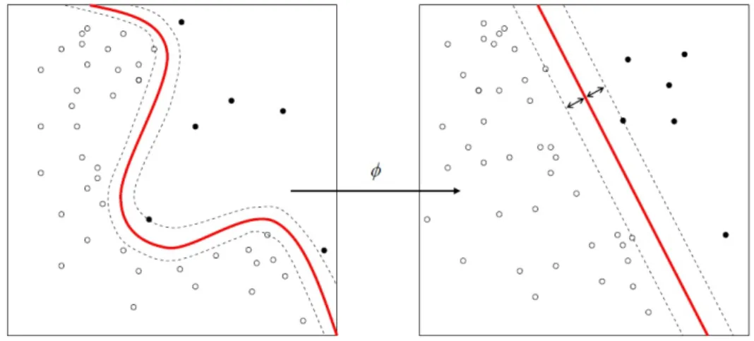
In some cases, it may be possible to map data which is not linearly separable into a

higher (possibly infinitely) dimensional space, where it is possible to linearly separate

the data6_{. See for example Figure 2.6, which shows how a function} _φ _{is used to map}

data to a space where the data is linearly separable, using an SVM approach in this case.

Figure 2.6: Non-linear Support Vector Machine7

It is possible to operate in this higher dimensional space without ever explicitly mapping the original data to the space by performing operations solely on inner products in the inner product space of this higher dimensional space, the so-called “kernel trick”[33]. There are a number of linear classifiers which can be adapted to take advantage of this to form non-linear classifiers, including LDA[24] and the SVM[9]. PCA[25] can also be

6_{http://www.youtube.com/watch?v=3liCbRZPrZA}

7_{http://en.wikipedia.org/wiki/File:KnnClassification.svg} 7

(31)

adapted to use this technique.

Unfortunately, the problem of finding a good kernel to use for a problem is non-trivial. A common initial choice of kernel is a Gaussian radial basis function:

K(xi,xj) = exp(−γkxi−xjk2) which has a single parameterγ >0.

2.8.10 Conservative Classifiers

An important thing to note is that the problem formulation allows classifiers to predict that more than one selection will win. Clearly this is impossible and so in situations like this, we will classify both selections as lose. This means that the recall of the classifier will decrease, but the precision will almost certainly increase as a result, which is well suited to the problem since we are most interested in the precision. This conservative attitude can be thought of as a kind of sanity check each classifier makes - “do I agree with myself?”.

2.8.11 Measuring Performance

Recall and Precision

In the case of the binary classifier predicting whether selections win or lose, there are four cases for the result of a classification, explained in Table 2.1.

Type Symbol Description

False Positive FP Predicted win, actual loss

False Negative FN Predicted loss, actual win

True Positive TP Predicted win, actual win

True Negative TN Predicted loss, actual loss

Table 2.1: Classification Cases The precision and recall quantities[26] are defined as:

Precision = _TP+FPTP and Recall = _TP+FNTP .

Precision represents the proportion of all win classifications made that were actual wins. Recall represents the proportion of all actual wins that were identified as wins by the classifier.

Perhaps the most important of these in a betting scenario is Precision, since it takes into account the false positive. The false positive is the only case where, if the advice of the classifier is taken, money is staked which will be lost. Precision of 1 corresponds toall

of the win classifications made being actual wins, whereas Precision of 0 corresponds to

none being actual wins.

However, Recall is also important since a higher Recall rate would correspond to a larger number of opportunities for winning bets to be placed.

(32)

Over-fitting

All of the classifiers considered use a training set to “learn” the structure of the data. Over-fitting refers to when the classifiers begin to become biased towards the training set; effectively learning the specifics of the random noise in the sample rather than learning a generalised model. As an extreme example, if number of parameters is the same as the number of examples, the classifier could end up “memorizing” the training data completely.

Equally, it is possible for a classifier to under-fit by being too general and not learning any of the important structure. This could happen if too few training examples were used for example.

As a result of this, rather than using a single training set and single testing set to evaluate performance, it makes more sense to use a technique such as cross validation to help avoid the possibility that classifiers may appear to be performing well by chance. In cross validation, the entire set of examples is randomly split intoN “folds”. A single

fold is then used as the testing set, whilst the remaining (N ₋1) folds are used as

the training set. This is repeated for each fold in turn and then the average of the performance measures (such as Precision and Recall) can be used to compare classifiers.

2.8.12 Learning Classifier Hyper-Parameters

Of the classifiers discussed, some have additional “tuning” parameters which must be chosen. For example, the linear SVM requires the soft margin parameter to be chosen. One way to make effective use of data available is to perform an axillary cross

vali-dation step within the main cross valivali-dation loop. For instance, when performing N

fold cross validation of a data set, for each of the N training sets, we can split this

intoM folds which are used to perform M fold cross validation for each of the possible

hyper-parameter configurations. The best performing configuration is then trained on

the wholeM folds and the outerN fold cross validation proceeds as usual. This is shown

in Figure 2.7.

The hyper-parameters to be determined for each classifier are shown in Table 2.2.

Classifier Parameters

KNN Number Of Neighbours

Linear SVM Soft Margin

Kernel SVM Soft Margin, Kernel Parameters

Naive Bayes Number Of Bins

Table 2.2: Summary Of Classifier Hyper Parameters

2.8.13 Summary

Both linear (LDA, SVM, Naive Bayes) and non-linear (logistic regression, KNN, kernel LDA, kernel SVM) methods for binary classification have been considered since it is

(33)

Figure 2.7: Auxiliary Cross Validation For Choosing Classifier Parameters

unclear which approach will perform best with the data being investigated.

The computational complexity of these methods for training and classification has not been taken into account at this stage. This is because the primary concern is to produce an accurate classifier which can be trained and classify new examples in a “reasonable” time, as opposed to having explicit upper bounds on the time that the classifier must

(34)

2.9. Sizing Bets Chapter 2. Background

take to be trained and classify new examples. However, if this does become a problem with the empirical data which is to be investigated, the issue will be revisited.

One of the frameworks considered (see Section 3.1.2) has implementations for the major-ity of the classifiers mentioned and so it was practical to experiment with almost all of the classifiers, however ultimately I decided to focus my investigation towards six types of classifier: linear discriminant analysis (LDA), Naive Bayes (NB), logistic regression (LR), weighted K nearest neighbour (WKNN) using an inverse distance weighting, and finally two support vector machine variants, with a linear kernel (LSVM) and Gaussian kernel (GSVM).

Many other types of binary classifier exist that have not been discussed, for example neural networks, decision trees and mixture models. These methods were not looked into further since they either appeared to be less suited to the problem or are known to be prone to over-fitting.

2.9 Sizing Bets

Given we have a way of assigning a classification to each new selection, this begs the question - how much should I bet when the classification is positive? One option is to bet a fixed amount every time. Another option could be to follow the crowd’s opinion on how much to bet, by using the average stake which was placed on the selection in question.

However, if we truly do have an edge over the odds being offered, there may be a more intelligent way to size our bets.

2.9.1 The Kelly Criterion

The Kelly criterion[21, 35] is a formula used to determine the optimal stake size in a series of bets. The strategy will perform better than any essentially different strategy in the long run, where the objective is increasing wealth.

Essentially, the strategy is equivalent to, given a choice of bets, to choose the one with the highest geometric mean of outcomes[4].

In the case of simple bets with two outcomes, either losing the stake amount or winning a profit according to the odds, the fraction of the current bankroll to stake is:

f∗ = p(v+ 1)−1 v

wherep is the win probability andv are the fractional odds being offered (“v to 1”).

This can be thought of as “expected profit divided by profit if you win”.

It is possible thatf∗ is negative (when the expected profit is negative) which means that no bet would be placed in this case.

Alternatives to the Kelly strategy include a fractional variant, where the proportion of the bankroll wagered is f_c∗ for some positive integer c. This can help reduce the short

(35)

2.9. Sizing Bets Chapter 2. Background

term volatility[37] of the strategy and also protect against bad estimates being made for

p, but at the cost of a reduced potential maximum return.

2.9.2 Return On Investment Simulations

Considering this, a novel way to look at the performance of the meta-tipster on the real world data could be to simulate a series of bets given an initial bankroll, where the classifier sizes its bets according to the (fractional) Kelly strategy.

This requires that the probability of winning is provided by the classifier, which is only available in the case of logistic regression and the Naive Bayes classifiers. For other classifiers, the probability of winning could simply be set to a fixed value, however this may not be very effective.

(36)

3

Implementation

In this chapter, details of the implementation side of the project are presented. Section 3.1 gives an overview of the various technologies used. Section 3.2 covers the approach taken to data storage and persistence. Section 3.3 explains how the real world data was collected. An overview of the simulated world system can be found in Section 3.4. Section 3.5 considers the implementation of the analysis side of the project and finally Section 3.6 discusses the approach taken to testing.

3.1 Technology Used

Throughout the course of the project I made use of a number of different technologies to facilitate the implementation. The following is a brief summary of how each was used.

3.1.1 Programming Language

The language I settled on to use was C# _{(C Sharp)}1_{. I made this decision because I}

found several libraries I thought would be useful to use which happened to be written in

C#_{and this was judged to be a better alternative than attempting to port such libraries}

to another language I was more familiar with.

I also made use of R2 _{towards the end of the project, due to its extensive library of}

statistics packages and as a means to present data using graphs and charts.

3.1.2 The Accord.NET Framework

The Accord.NET framework3 _{is a C}_#_{framework which extends the AForge.NET}

frame-work4_{. It contains implementations of many of the machine learning and statistics}

1_{http://msdn.microsoft.com/library/z1zx9t92} 2_{http://www.r-project.org/}

3

http://accord-net.origo.ethz.ch/

(37)

3.1. Technology Used Chapter 3. Implementation

techniques that were explored, including PCA, LDA, SVM, kernel variants, logistic re-gression and hypothesis testing.

3.1.3 Math.NET Numerics

The Math.NET Numerics C# _library5 _{contains implementations for a variety of}

differ-ent discrete and continuous distributions, some of which are not yet implemdiffer-ented in Accord.NET.

3.1.4 ALGLIB

The ALGLIB numerical analysis library6 _{contains implementations for PCA, LDA and}

logistic regression. It was considered as a possible alternative to Accord.NET, however it does not have as much functionality, for example no kernel variants of the PCA and LDA algorithms.

3.1.5 Emgu CV

Emgu CV7 _{is a C}_#_{wrapper for the OpenCV}8 _{image processing library. It was used as}

an alternative to the Accord.NET SVM implementation after it was found that it was

poorly optimised. The SVM implementation in OpenCV is based on LIBSVM9_.

3.1.6 NHibernate

NHibernate10 _{is an object-relational mapper for C}_#_{which can be used to abstract away}

the database access layer. This is used as an alternative to interacting directly with the database so that the implementation code is not directly tied to the underlying database used.

In addition, Fluent NHibernate11_{was used to avoid using XML files to define mappings}

so that the mapping code remained compile safe.

3.1.7 SQLite

SQLite12_{is a library which implements a self contained SQL database engine, allowing a}

databases to be stored to a single portable file. The advantage of this is that, for example, the different data sets that will be simulated or collected could each be persisted to an

5_{http://www.mathdotnet.com/} 6 http://www.alglib.net/ 7_{http://www.emgu.com/wiki/index.php/Main_Page} 8_{http://opencv.willowgarage.com/wiki/} 9 http://www.csie.ntu.edu.tw/~cjlin/libsvm/ 10_{http://nhforge.org/Default.aspx} 11_{http://www.fluentnhibernate.org/} 12_{http://www.sqlite.org/}

(38)

3.2. Persistence Chapter 3. Implementation

individual database file. It is also possible to use SQLite in memory, which helps facilitate unit testing of database code. SQLite was used as the back end storage mechanism.

3.1.8 Html Agility Pack

The Html Agility Pack13 _{is a HTML parser library for C}_#_{which can be used for parsing}

the web pages scraped as part of the data collection process. This is used as an alternative to, for example, direct use of regular expressions to parse HTML, which can lead to unpredictable, hard to maintain code14_.

3.1.9 NUnit

NUnit15 _{is a C}_# _{unit-testing framework which was used to write unit tests for the}

im-plementation, an important part of any software development.

3.2 Persistence

One of the first steps I took was to figure out how best to store the data that I would be both simulating and collecting from tipping websites. I decided to use a relational database for this, which meant I had to first figure out the design and then consider how to interface with C#_.

3.2.1 Database Design

Figure 3.1 shows the relationships between the main data entities. These were designed so that each entity corresponds to a table in the database and also to a class in the object oriented implementation. The design allows any “sport” imaginable to be represented; a sport is assumed to be a type of event for which matches are played by participants of the sport, referred to as runners. For each match, a number of different markets may be available. For a particular available market, there will be a number of possible outcomes for that market, referred to as selections, each corresponding to a runner for the sport in question.

To put this in perspective, for the case of tennis, specifically the tennis win market, the runners are the tennis players and for each tennis match played there will be a win market available for the match, for which the two participants in the tennis match will be the possible outcomes for the market. Tipsters who belong to a site, say TennisInsight members, can then tip matches according to who they predict will win each match.

13_{http://htmlagilitypack.codeplex.com/}

14_{http://www.codinghorror.com/blog/2009/11/parsing-html-the-cthulhu-way.html} 15_{http://nunit.org/}

(39)

3.2. Persistence Chapter 3. Implementation

Figure 3.1: Relationships Between Main Data Entities

3.2.2 Persistence Layer

I was careful to make sure that the layer between the database and the programming language was not tightly coupled; I wanted to make it easy to use a different storage implementation in the future. To achieve this, I used NHibernate.

I found getting used to NHibernate a challenge at first and it took a lot longer than expected to get everything “just working”. However, after overcoming this, aided by the excellent NHibernate 3.0 Cookbook[11], I found that the persistence layer did exactly what I wanted it to and I could now talk about my entities in terms of objects in the programming language, without having to worry about the intricacies of how they would

(40)

3.3. Scrapers Chapter 3. Implementation

actually be persisted.

3.2.3 Storage Mechanism

I decided to make use of the SQLite database engine as the back end storage mechanism, mainly for the convenience of not having to run a full blown database server instance, although a different database could be “swapped in” at any time due to the fact that the persistence layer abstracts away the underlying storage mechanism. Another benefit of SQLite is that it allows you to use entirely in-memory database instances, which was useful for running simulations which did not need to be persisted, as well as for unit testing purposes.

3.3 Scrapers

After setting up the persistence later, the next step was to collect the real-world data. I did this early on in the project since it was possible that the websites would later become unavailable.

I encountered problems when attempting to gather data from OLBG, since the site had a particularly sensitive flood detection, which meant it was not feasible to scrape the data in good time. In addition, only 45 days of tip history were available, whereas TennisInsight had tip histories going as far back as 2008 available. As such, I focused on TennisInsight, where I did not encounter any problems collecting the data.

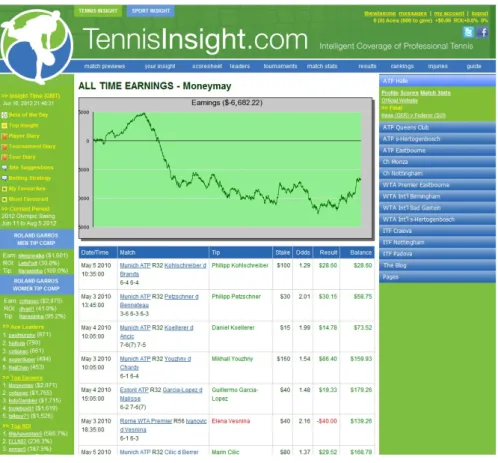
3.3.1 TennisInsight

The main data to be scraped from TennisInsight was the tip histories of all of the tipsters. These tip history pages used plain HTML which made it possible to learn the structure of the pages and extract the relevant information. An example of a tip history page is shown in Figure 3.2.

I decided to use a HTML parser library rather than directly attempting to use regular expressions. This was for two reasons, firstly regular expressions can be hard to maintain (“what does that do again..?”). Secondly, if pages did not appear how I expected them to, using a library allowed me to use exception handling to make sure I was not populating the database with garbage! On several occasions this appeared to be a good decision; some pages served up contained bad structure, for example missing closing HTML tags.

Unexpectedly, I also managed to discover amajor security flaw on the site which meant

thatany user’s password and personal details were publicly viewable in plain text! The

issue was reported to the site owner and has since been fixed.

The scraper made use of a separate worker thread for saving the downloaded pages to disk so that disk access was not a bottleneck. Scraped pages to save were queued up in a string representation and the worker thread would continuously check for new work on the queue to be saved.

(41)

3.4. Simulated World Chapter 3. Implementation

Figure 3.2: TennisInsight Tip History Page Example

3.4 Simulated World

With my scraper now populating the database with the thousands of tips on TennisIn-sight, I now turned my attention to implementing the simulated world. The idea was that simulations would be persisted in the same way that the real-world tips were, so that the analysis side of the implementation is completely decoupled from the method which was used to generate/collect the data to be analysed.

3.4.1 System Overview

A simplified overview of the simulation system is shown in Figure 3.3. The Simulation-Constructor uses a SimulationSpecification to construct the simulation, which it may then persist if required. The design of the simulated world in the background section translated almost directly; each tipster has a strategy comprising of three components, estimation, selection and stake.

(42)

3.4. Sim ulated W orld Chapter 3. Implemen tation

Figure 3.3: Simulation System Overview