LAIM discretization for multi-label data

LAIM discretization for multi-label data

Alberto Canoa,b_{, Jos´e Mar´ıa Luna}b_{, Eva L. Gibaja}b_{, Sebasti´an Ventura}b,∗

a

Dpt. of Computer Science, Virginia Commonwealth University, Richmond, VA, USA

b

Dpt. of Computer Science and Numerical Analysis, University of Cordoba, Spain

Abstract

Multi-label learning is a challenging task in data mining which has attracted growing attention in recent years. Despite the fact that many multi-label datasets have continuous features, general algorithms developed specially to transform multi-label datasets with continuous attributes’ values into a fi-nite number of intervals have not been proposed to date. Many classification algorithms require discrete values as the input and studies have shown that supervised discretization may improve classification performance. This pa-per presents a Label-Attribute Interdependence Maximization (LAIM) dis-cretization method for multi-label data. LAIM is inspired in the discretiza-tion heuristic of CAIM for single-label classificadiscretiza-tion. The maximizadiscretiza-tion of the label-attribute interdependence is expected to improve labels prediction in data separated through disjoint intervals. The main aim of this paper is to present a discretization method specifically designed to deal with multi-label data and to analyze whether this can improve the performance of multi-label learning methods. To this end, the experimental analysis evaluates the per-formance of 12 multi-label learning algorithms (transformation, adaptation, and ensemble-based) on a series of 16 multi-label datasets with and without supervised and unsupervised discretization, showing that LAIM discretiza-tion improves the performance for many algorithms and measures.

Keywords: Multi-label learning, data discretization

∗_{Corresponding author}

Email addresses: [email protected](Alberto Cano),[email protected]

(Jos´e Mar´ıa Luna), [email protected](Eva L. Gibaja),[email protected]

1. Introduction

The machine learning community has studied the classification task in depth. The usual way to define this task involves associating one class la-bel with each pattern. It can be distinguished between binary and multi-class multi-classification. In the former only two multi-classes are defined, indicating if the pattern belongs or not to the target whilst in the latter more than two classes are defined. This classical definition of the task entails the only-one-label-per-pattern restriction. Nevertheless there are more and more current classification problems, such as text and sound categorization, semantic scene classification or gene and protein function classification, in which a pattern could have simultaneously associated not one but a set of labels. These prob-lems with multiple outputs entail specific difficulties such as the exponential growth of combinations of labels to take into account, label correlations and even data imbalance. All of these factors have lead to the emerging of Multi-Label Learning (MLL) paradigm [21, 60]. In contrast to classical (a.k.a. single-label) learning, MLL is able to address problems where class labels are not mutually exclusive. First applications of MLL were related to clas-sification of text and multimedia [45, 46], in which one document or picture could be simultaneously associated with several categories, and protein and gene function classification, in which a gene or protein can perform several functions [59]. Nowadays MLL has become a challenging research area with an increasing number of papers and domains of application such as drug discovery [24], social network mining [27], and direct marketing [61].

On the other hand, many machine learning and statistical techniques have been designed to learn only in datasets composed of nominal variables while real-world applications usually involve continuous features [26, 29]. In order to overcome this drawback one solution is to use an embedded or external method to discretize continuous features by partitioning them into a number of discrete intervals and treat each one as a category. As it maps from a high dimensional range of values to a reduced subset of discrete values, discretizacion can be considered a data reduction method [20]. Obtaining the optimal discretization is NP-complete [10] being a potential time-consuming bottle-neck.

Despite the fact that many multi-label datasets have continuous features, general algorithms developed specially to transform multi-label datasets with continuous attributes’ values into a finite number of intervals have not been proposed to date. Studies have shown the advantages of supervised

dis-cretization [20] and many classifiers require discrete input. This paper presents a discretization approach based on Label-Attribute Interdependence Maxi-mization (LAIM) that can be applied to numerical multi-label datasets. The proposal is inspired on the CAIM [28] discretization method for multi-class single-label classification and extends its application to multi-label data. The label-attribute interdependence maximization is expected to improve the generation of discrete intervals that boost the performance of subsequent multi-label classifiers. The primary objective of this paper is to present a supervised discretization method specifically designed for multi-label data and to analyze whether multi-label discretization can improve performance of state-of-art MLL algorithms. The experimental study evaluates and com-pares the performance of 12 multi-label algorithms (transformation, adapta-tion, and ensemble-based) with and without discretization on 16 datasets. Moreover, 13 different metrics are used to evaluate the performance of the algorithms. The experimental results are contrasted through the analysis of non-parametric statistical tests [19], namely the Wilcoxon [54] test that evaluates whether there are statistically significant differences between the performance of algorithms on discretized and non-discretized data.

The paper is structured as follows. Section 2 reviews related works on multi-label and data discretization. Section 3 describes the LAIM discretiza-tion method to multi-label data. Secdiscretiza-tion 4 presents the experimental study and Section 5 discusses the results and the statistical analysis. Finally, Sec-tion 6 shows the main conclusions of this work.

2. Background

In order to provide the reader with the necessary background, this section presents an overview of both MLL and discretization techniques.

2.1. Multi-label learning

Given F = F1 ×. . .×Fk a k-dimensional input space of numerical or

categorical features, and an output space of q labels, Y = {λ1, λ2, . . . , λq},

in MLL an instance has the form (x, Y), where x = (x1, . . . , xk) ∈ F, and

Y ⊆ Y is called labelset. Label associations can be also represented as a q dimensional binary vector y= (y1, y2, ..., yq) ={0,1}q where each element is

1 if the label is relevant and 0 otherwise. Note that in single-label learning each example has the form (x, y), where x= (x1, . . . , xk)∈ F, and y∈ Y.

MLL problems can be dealt from two points of view [48]. On the one hand some studies have proposed transformation methods, which transform an original multi-label problem into one or several single-label problems, which will then be resolved using a classical classification algorithm. On the other hand, there are studies proposing the extension of classical classification paradigms to cope with multi-label data directly; these are called algorithm adaptation methods.

Some transformation methods are based on label combinations. Thus, the Label Powerset (LP) [48] method considers each combination of labels in the original dataset as a new and different label. The main drawback of LP is its complexity, that grows exponentially with the number of labels. The

Pruned Sets (PS) [40] method is similar to LP but specifically designed for problems with a large number of label combinations. Therefore, PS prunes the patterns associated with the less frequent combinations and after that, it reintroduces the pruned examples along with frequent subsets of their label sets. Ensemble of Pruned Sets (EPS) [42] constructs a number of PS by sampling the training sets (i.e. boostrap). The RAkEL algorithm [49] produces several LP classifiers, which are specialized in classifying random subsets of labels. Answers are combined by a voting process.

Other transformatin methods are based on binary decompositions of the problem. Binary Relevance(BR) [48] generates one independent binary clas-sifier for each label, the positive patterns being the ones belonging to the label, and being the rest negative patterns. The final output of the multi-label classifier is obtained by combining the outcomes of all of the classifiers. The main problem of BR is the independence assumption. Classifier Chains

(CC) [43] also generates q binary classifiers, but they are linked in such a way that the feature space of each link in the chain is extended with the labels associations of all previous links. Thus, CC overcomes the label inde-pendence assumption of BR and the potentially computational complexity of LP. Ensemble of Classifier Chains (ECC) trains a set of CC classifiers with a random chain ordering and a random subset of training patterns. Depen-dent Binary Relevance (DBR) [35] also follows a binary decomposition but incorporating, for each binary classifier, the information of the rest of labels as additional features.

Calibrated Label Ranking (CLR) [5] carries out a pairwise decomposition and produces a binary model for each pair of labels. Besides, it adds a virtual label that is used as a splitting point between positive and negative labels.

al-gorithms have been adapted to deal with multi-label data directly, with-out pre-processing the multi-label dataset. For instance, decision trees [11], SVMs [34, 52], associative classification [39] or bio-inspired approaches [1]. It is worth citing Multi-label k-nearest neighbor (MLkNN) [58]. It first de-termines the k nearest neighbors and then, based on prior and posterior probabilities for the frequency of each label within the k nearest neighbors, it identifies the set of labels to be associated to the unknown example by using the maximum a posteriori principle. Instance Based Learning by Lo-gistic Regression (IBLR) [8] is an approach that combines instance-based learning and logistic regression. Together with MLkNN it can be considered state-of-the-art in MLL by instance based approaches.

Ensemble methods whose base classifiers are multi-label learners (i.e. EPS, ECC, RAkEL) are considered in [33] a special group of methods because they are developed on top of problem transformation and algorithm adap-tation approaches. Hierarchy Of Multilabel classifiERs (HOMER) [47], that generates a tree of multi-label classifiers is also included in this group. The root node represents all labels and the tree is top-down generated. At each node a balanced clustering algorithm groups similar labels into a meta-label

and then a multi-label learner is built to predict these meta-labels. Table 6 summarizes the methods that have been considered in this paper and the configuration recommended by its authors.

2.2. Data discretization

The goal of discretization is to find a set of cut points to partition the range of values of a numerical feature into a small number of intervals that have good class coherence, which is usually measured by an evaluation func-tion. A recent taxonomy of discretization methods has been proposed in [20]. A common criteria to classify discretization issupervised vs. unsupervised de-pending on whether the class information is taken or not into account by the classifier. Other criteria (e.g. global vs. local, static vs. dynamic, univariate vs. multivariate) have been described in [20].

Two representative unsupervised algorithms are Equal-width (EW) and

Equal-frequency (EF) discretizations [37]. The former divides the range of values for an attribute into a number of equal sized bins. The latter divides the continuous attribute into a number of bins so that each bin contains approximately the same number of training instances. In both cases, the number of bins is provided by the user. Unsupervised discretization methods ignore important information: the labels of the class attribute.

Most discretizers in literature are supervised and use class information to determine the best number of intervals. There are some methods based on the χ2

statistic that focus on the statistical point of view. Thus, ChiMerge [25] is a bottom-up method that starts from the set of single value intervals and iteratively merge neighboring intervals. The top-down method based on χ2

is ChiSplit [32]. Entropy-based methods focus on the information theoretical point of view [13, 23, 30]. Fayyad and Irani [18] presented an entropy-based method that used the class information entropy of candidate partitions to select boundaries for discretization. Finally, CAIM [28] is a top-down discretization algorithm that maximizes the interdependence between class labels and attribute values while minimizes the number of intervals.

Up to our knowledge, data discretization has not received too much at-tention in the field of multi-label learning to date and specific algorithms for multi-label data discretization have not been proposed. Only a few works cite any pre-processing of multi-label data that is carried out in order to fit the inputs to specific algorithms in particular fields, which are detailed next. In [16] for each continuous feature, the values were sorted and then every four consecutive values were treated as one interval. As this method is un-supervised the label information was ignored, besides the method was used in a specific problem (i.e. protein fold prediction) and with a specific algo-rithm. In [2] each label was pre-processed with class-attribute contingency coefficient [9] due to the fact that the proposed MLL method (based on Bayesian networks) was defined for discrete variables. As the class-attribute contingency coefficient is a method defined for standard classification, its application on multi-label data may cannot generate the most appropriate discretization intervals . Besides, the two cited works did not study the ef-fect of discretization on the performance of the proposals. Finally, in [36], two supervised entropy-based discretization algorithms were proposed in or-der to explore the potential of weighted representations of documents (e.g.

tf*idf) in the context of AdaBoost-like algorithms that required documents to be represented by binary vectors. These methods were based on informa-tion gain and split a continuous feature into two discrete intervals. As the criteria used was multi-class they binarized the attribute domain without any further consideration of the labelset distribution. There is no general knowledge on whether data discretization may improve the performance of multi-label learning algorithms. Consequently, it is our objective to truly ex-plore in this paper the potential benefits and advantages of multi-label data discretization as measured by the performance of a set of MLL algorithms.

Class Interval Class Count [d0, d1] ... (dr−1, dr] ... (dn−1, dn] λ1 m11 ... m1r ... m1n M1•=P M j=1Jλ1=yjK : : ... : ... : : λi mi1 ... mir ... min Mi•=P M j=1Jλi=yjK : : ... : ... : : λq mq1 ... mqr ... mqn Mq•=P M j=1Jλq =yjK Interval Total M•1 ... M•r ... M•n M

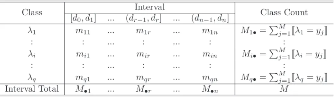
Table 1: Single-label quanta matrix for attributeF and discretization schemeD 2.3. CAIM discretization for single-label data

CAIM is a supervised discretization algorithm whose goal is automatically selecting both the number of discrete intervals and the cut points based on the interdependency between class and attribute values maximization. In or-der to achieve such a goal, theClass-Attribute Interdependency Maximization

is used as the criterion for optimal discretization. In addition, a secondary goal is to minimize the number of intervals without significant loss of class-attribute mutual dependence. The definition of CAIM for classical single-label learning is the following. Given a dataset of M instances where each example belongs to one ofqpredefined classes. CAIM discretizes the continu-ous attributeF intondiscrete intervalsD={[d0, d1],(d1, d2], . . . ,(dn−1, dn]}

where d0 is the minimal value, dn is the maximal value and dv < dv+1, for

v = 0,1, . . . , n−1. Such a discrete resultD is called a discretization scheme on attribute F being P ={d1, d2, . . . , dn−1}the set of cut points [20].

If the class variable and the attribute are treated as two random variables, a two-dimensional frequency matrix (a.k.a. quanta matrix) can be obtained as shown in Table 1, where M is the number of instances, M_i• is the number of instances belonging to class λi and M•r is the number of instances in the

interval r. Therefore, mir is the number of instances in the interval (dr−1, dr]

belonging to class λ_i. For any predicate π, JπK returns 1 if the predicate is true and 0 otherwise.

The CAIM criterion measures the dependency between the data classes and the discretization scheme D for an attribute F. It is specified in Equa-tion 1 where n is the number of intervals, r iterates over all intervals, maxr

is the maximum value among all mir values (maximum value within the rth

column of the quanta matrix), M_•r is the total number of instances that are within the interval (dr−1, dr] of attribute F. The larger the value of CAIM,

the higher the interdependence between the class labels and the discrete in-tervals, and consequently, the better subsequent classification [6].

CAIM(D|F) = Pn r=1 max2 r M•r n (1)

3. LAIM discretization for multi-label data

This section presents the LAIM discretization algorithm for multi-label data. LAIM is inspired on the CAIM discretization for single-label discretiza-tion but extended to deal with multi-label data by taking into account the whole labelset of the instances instead of the single-label class of original CAIM. This way, based on the labelset and the discretization scheme it can be defined a multi-label quanta matrix, which is shown in Table 2.

In contrast to the the single-label quanta matrix, there are differences in the counts of the sum of rows and columns based on the labels information. In this case, M_i• =PM_j=1Jλ_i ⊆ Y_jK, is the number of instances in which the labelλi is positive. M•r is the total number of positive labels that are within

the interval (dr−1, dr] of attribute F. Importantly, unlike the single-label

case, the sum of the right column will be not the number of instances but the total number of positive labels in the whole dataset PM_j=1|Yj|.

This definition of a multi-label quanta matrix can be employed by any discretization algorithm to adapt its methodology to handle multi-label data appropriately. The LAIM criterion is specified in Equation 2 where n is the number of intervals, riterates over all intervals, maxr is the maximum value

among all m_ir values (maximum value within the rth column of the multi-label quanta matrix), M_•r is the number of positive labels that are within

the interval (dr−1, dr] of attribute F, and PM_j=1|Yj| is the total number of

positive labels. The LAIM criterion is an adaptation of the CAIM’s in Equa-tion 1 for multi-label data as it measures the dependency between the labels and the discretization scheme D for an attribute F. The numerator of the equation maximizes the relation between the maximum number of examples having the same label divided by the total amount of labels happening each discretized interval. The denominator of the equation measures the total number of labels and intervals. Therefore, it is expected to maximize the relation between the numerator and the denominator. The larger the value of LAIM, the higher the interdependence between the labels and the discrete intervals.

Label Interval Label Count [d0, d1] ... (dr−1, dr] ... (dn−1, dn] λ1 m11 ... m1r ... m1n M1•=P M j=1Jλ1⊆YjK : : ... : ... : : λi mi1 ... mir ... min Mi•=P M j=1Jλi⊆YjK : : ... : ... : : λq mq1 ... mqr ... mqn Mq•=P M j=1Jλq ⊆YjK Interval Total M•1 ... M•r ... M•n P M j=1|Yj| Table 2: Multi-label quanta matrix for attributeF and discretization schemeD

Algorithm 1 LAIM algorithm

Require: Data consisting ofM examples,qlabels, a set of continuous attributesF

1: for allFi inF do

2: {Step 1: Initialization}

3: Find maximum,dn, and minimum,d0, values ofFi 4: Sort the continuous values ofFi in ascending order

5: FormB, the set of candidate interval boundaries, withd0,dnand all the mid points of all the adjacent pairs

6: Di= [d0, dn] 7: GlobalLAIM= 0 8: {Step 2: Discretization} 9: nIntervals= 1

10: for allbj ∈B do

11: Add a midpoint,bj, intoB which is not still inDi 12: CalculateLAIM value

13: end for

14: Accept the midpoint,bj, with highest value of LAIM 15: if LAIM > GlobalLAIM then

16: Di=Di∪midpoint 17: GlobalLAIM=LAIM

18: else

19: return Discretization schemeDi

20: end if 21: nIntervals=nIntervals+ 1 22: Go to line 10 23: end for LAIM(D|F) = Pn r=1 max2 r M•r n·PM_j=1|Yj| (2)

LAIM algorithm (listed in Algorithm 1) uses a greedy approach. It begins with a single interval that covers all possible values of a certain attribute and divides it iteratively by choosing the midpoint that yields the highest value of LAIM criterion. This process is repeated until the LAIM value is no further improved, i.e., the LAIM value with k intervals is lower than with k −1 intervals. The intrinsic behavior of the LAIM criterion advocates for a small number of intervals because in Equation 2 (which has to be maximized) the denominator includes the number of intervals. Therefore, when the algorithm follows a top-down greedy approach it is more likely to keep discretization schemes with smaller number of intervals rather than splitting the attribute’s domain generating a very large number of intervals that eventually decrease the LAIM value.

4. Experiments

This section presents experimental setup to detail the performance evalu-ation metrics, the multi-label datasets, the algorithms and their experimental settings. Detailed results of the experiments are available in the website1

.

4.1. Evaluation metrics

Performance metrics used in MLL can be categorized intolabel-based and

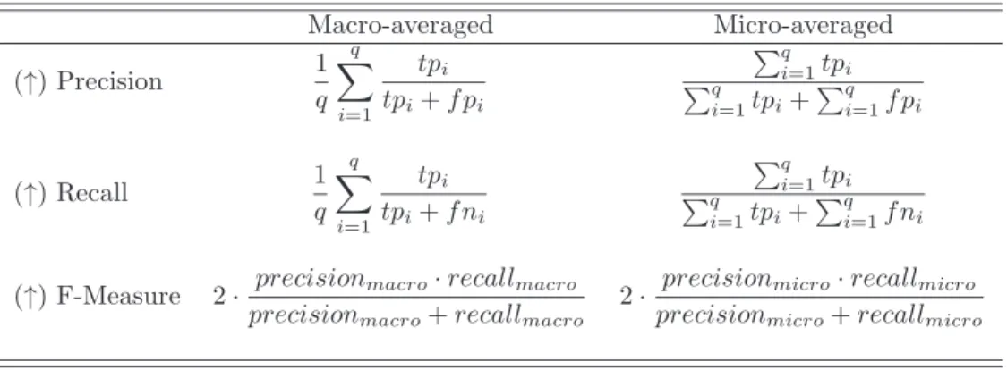
example-based. Label-based metrics compute a binary performance metric based on the contingency: table true positives (tp), true negatives (tn), false positives (f p) and false negative (f n) values. Due to the fact of having a contingency table for each label, macro and micro averaging methods can be used [49]. The macro approach calculates the binary metric for each label and these values are then averaged. On the other hand, the micro ap-proach aggregates the values of all contingency tables to finally compute the metric. According to [38] and [57], macro averaging gives all the labels the same weight being better when the system is required to perform consistently across all labels regardless their frequency, while micro averaging tend to be more influenced by common labels. In this work macro and micro preci-sion, recall and F-measure have been considered and are defined in Table 3

1 _{Datasets and detailed results for all metrics and algorithms are fully described and} publicly available to facilitate the replicability of the experiments and future comparisons at the website: http://www.uco.es/grupos/kdis/wiki/MLdiscretization

Macro-averaged Micro-averaged (↑) Precision 1 q q X i=1 tpi tpi+f pi Pq i=1tpi Pq i=1tpi+P q i=1f pi (↑) Recall 1 q q X i=1 tpi tpi+f ni Pq i=1tpi Pq i=1tpi+P q i=1f ni (↑) F-Measure 2· precisionmacro·recallmacro

precisionmacro+recallmacro

2· precisionmicro·recallmicro

precisionmicro+recallmicro

Table 3: Label-based evaluation metrics

where (↓) indicates the smaller the value the better the performance and (↑) indicates the larger the value the better the performance.

On the other hand, example-based metrics compute a metric for each instance an then this value is averaged across all instances. Example-based metrics are shown in Table 4. Let a multi-label dataset consisting of M examples, each one associated with a set of labelsY ⊆ Y. The classifier pre-dicts a set of labels Z for each example. The subset accuracy [62] computes the percentage of instances whose predicted labels are exactly the same as their corresponding set of ground-truth labels. As an exact match between the predicted and the true sets of labels is needed it is considered a very strict evaluation measure. The Hamming loss [45] considers the prediction error (an incorrect label is predicted) and missing error (a label is not pre-dicted) at the same time, being ∆ the symmetric difference of two sets and corresponds to the XOR operation in boolean logic. The smaller the value of Hamming loss, the better the performance. Accuracy, precision, recall, and F-measure have been also defined as example-based metrics. Finally, the ranking loss [21] is a ranking metric that evaluates the average fraction of label pairs that are disordered for an example. The goal is to obtain a small number of misorderings so that the labels in Y are ranked above the ones in Y where |E| is called the error-set-size in [12] and it is defined as

E =

(λ, λ′_)|τ

i(λ)> τi(λ′),(λ, λ′)∈Yi×Yi where τ_x∗ is the true ranking. 4.2. Datasets

A set of numerical multi-label datasets has been used in the experiments to evaluate the performance of the proposal and compare to other methods. They are called CAL500 [51], Emotions [46], Birds [4], Flags [22], Scene [3]

(↓)Hamming loss= 1 M M X i=1 |Yi∆ Zi| q (↓)Ranking loss= 1 M M X i=1 1 |Yi||Yi| |E| (↑)Subset accuracy= 1 M M X i=1 JZi=YiK (↑)Accuracy= 1 M M X i=1 |Yi∩Zi | |Yi∪Zi | (↑)P recision= 1 M M X i=1 |Yi∩Zi| |Zi| (↑)Recall= 1 M M X i=1 |Yi∩Zi| |Yi|

(↑)F−M easure= 2· precision·recall

precision+recall

Table 4: Ranking and example-based evaluation metrics

and Yeast [17], Tmc2007-500 [49], Human [55], Plant [55], a set of Yahoo!

datasets [52] and Rcv1v2 [31]. These datasets belong to a wide variety of application domains and they have been used in other studies covering several paradigms. For datasets Yahoo! and Rcv1v2, theχ2

feature ranking method proposed in [49] was used separately for each label, and the top 500 features based on their maximum rank over all labels were selected.

These datasets have been collected from the MULAN [50], MEKA [41] and LABIC [56] repository websites and they are very varied in their degree of complexity, number of labels, number of attributes, and number of examples. The number of labels ranges from 6 to 174, the number of attributes ranges from 19 to 500, and the number of examples ranges from 194 to 11214. Datasets were partitioned using the 10-fold cross validation procedure [53].

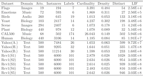
Table 5 summarises the information about these datasets. Items in the table have been ordered according a somewhat rough overall complexity mea-sure used by Read [43], consisting of the product of labels ×instances×

attributes (we refer it as LIF). The horizontal line separates large datasets. Thus, the label cardinality is the average number of labels of the examples in the dataset whereas the label density is the average number of labels of the examples in the dataset divided by q. Distinct is the total number of unique label combinations in the dataset.

Dataset Domain Atts. Instances Labels Cardinality Density Distinct LIF Flags Images 19 194 7 3.391 0.484 54 2.58E+4 Emotions Music 72 593 6 1.868 0.311 27 2.56E+5 Birds Audio 260 645 19 1.013 0.053 133 3.18E+6 Yeast Biology 103 2417 14 4.237 0.302 198 3.48E+6 Scene Images 294 2407 6 1.073 0.178 15 4.24E+6 Plant Biology 440 978 12 1.078 0.089 32 5.16E+6 CAL500 Music 68 502 174 26.043 0.149 502 5.94E+6 Human Biology 440 3106 14 1.185 0.084 85 1.91E+7 Yahoo(A.) Text 500 7484 26 1.653 0.063 599 9.72E+7 Yahoo(H.) Text 500 9205 32 1.644 0.051 335 1.47E+8 Yahoo(B.) Text 500 11214 30 1.598 0.053 233 1.68E+8 Rcv1(S1) Text 500 6000 101 2.879 0.028 1028 3.03E+8 Rcv1(S2) Text 500 6000 101 2.634 0.026 954 3.03E+8 Rcv1(S3) Text 500 6000 101 2.614 0.025 939 3.03E+8 Rcv1(S4) Text 500 6000 101 2.483 0.024 816 3.03E+8 Rcv1(S5) Text 500 6000 101 2.642 0.026 946 3.03E+8

Table 5: Description of the datasets

Cardinality= 1 M M X i=1 |Yi | Density = 1 M M X i=1 | Yi | q (3)

4.3. Algorithms and experimental settings

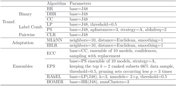
For the experimentation, we have evaluated the multi-label LAIM method with 12 different algorithms from the state-of-art and 16 datasets by using a 10-fold cross validation. The use of multiple algorithms belonging to different families pursue to avoid the bias a particular method to the experimentation. This way, we can evaluate the true impact of multi-label discretization on the behavior of multiple algorithms. Furthermore, the unsupervised Equal-width and Equal-frequency methods are included for comparison. The implemen-tation of these algorithms is available from the MULAN library [50] and they are summarized in Table 6. Parameters were set with the values recom-mended by the authors of each algorithm at their respective articles, or the provided by the MULAN software otherwise. The use of J48 as base classi-fier is commonplace in multi-label learning [60] and the same parameters are used in all the configurations.

Algorithm Parameters Transf. Binary BR base=J48 DBR base=J48 CC base=J48

Label Comb. LP base=J48, threshold=0.5

PS base=J48, apInstances=3, strategy=A, abInfreq=2 Pairwise CLR base=J48

Adaptation MLkNN neighbors=10, distance=Euclidean, smoothing=1 IBLR neighbors=10, distance=Euclidean, smoothing=1

Ensembles

ECC base=CC, ensemble of 10 models, confidences, sampling with replacement

EPS

base=PS ensemble of 10 models, strategy=A,

keeping the topb= 2 ranked subsets 66% data sample, threshold=0.5, pruning sets occurring lessp= 3 times RAkEL base=LP(J48), k=3, nmodels= 2×q, threshold=0.5 HOMER base=BR(J48), numClusters=3

Table 6: Parameters used by the algorithms. J48 confidenceFactor=0.25, pruning=true.

5. Results

This section presents the experimental results and discusses the perfor-mance of the algorithms based on non-parametric statistical analysis.

The 12 multi-label classification algorithms were run with and without data discretization and the results about the cross validation were gathered for each of the 13 performance metrics. One performance table was obtained for each metric considered. Besides, for each metric, a ranking of algorithms was built following the philosophy of the Friedman test [15] where the al-gorithm with the best value metric in one dataset is given a rank of 1 for that dataset, the algorithm with the next best metric value has the rank of 2, and so on. Finally, the average ranks of each algorithm in all datasets are calculated. These ranks let us know which algorithm obtains the best results across all datasets. In this way, the algorithm with the value closest to 1 indicates the best performance across most datasets.

Due to the article’s space limitations and the large number of datasets, metrics and methods employed, we show in the manuscript the results of the Hamming loss, ranking loss and subset accuracy, as they are the most popular and commonly employed metrics. On the other hand, full tables with all the results of the cross validation for each dataset (16), metric (13) and method (12) are available online for the readers in the website of the KDIS research group at http://www.uco.es/grupos/kdis/wiki/MLdiscretization

Algorithm Bir d s C A L 5 0 0 E m o ti o n s F la g s S c e n e Y e a st H u m a n P la n ts Y a h o o (A .) Y a h o o (B .) Y a h o o (H .) R c v 1 (S 1 ) R c v 1 (S 2 ) R c v 1 (S 3 ) R c v 1 (S 4 ) R c v 1 (S 5 ) A v e ra g e ( ↓ ) A v g .R a n k ( ↓ ) BR 0.050 0.162 0.252 0.256 0.132 0.249 0.123 0.139 0.055 0.025 0.032 0.029 0.025 0.026 0.023 0.025 0.100 24.31 BR-LAIM 0.045 0.141 0.243 0.261 0.130 0.232 0.099 0.101 0.054 0.024 0.032 0.027 0.023 0.024 0.022 0.024 0.093 14.34 BR-EW 0.047 0.146 0.239 0.263 0.150 0.220 0.097 0.104 0.057 0.026 0.041 0.027 0.024 0.024 0.022 0.023 0.094 20.34 BR-EF 0.050 0.140 0.245 0.249 0.143 0.220 0.085 0.090 0.055 0.025 0.034 0.027 0.024 0.023 0.022 0.023 0.091 14.91 DBR 0.051 0.163 0.273 0.277 0.177 0.283 0.231 0.239 0.150 0.027 0.044 0.032 0.027 0.029 0.031 0.032 0.129 40.75 DBR-LAIM 0.047 0.148 0.259 0.286 0.156 0.255 0.235 0.248 0.149 0.025 0.043 0.029 0.025 0.028 0.029 0.026 0.124 33.97 DBR-EW 0.046 0.148 0.264 0.290 0.270 0.241 0.302 0.326 0.264 0.028 0.051 0.030 0.024 0.025 0.022 0.025 0.147 34.50 DBR-EF 0.050 0.149 0.287 0.298 0.392 0.257 0.619 0.407 0.126 0.026 0.043 0.029 0.025 0.024 0.022 0.025 0.174 34.66 LP 0.062 0.201 0.258 0.293 0.146 0.278 0.127 0.141 0.070 0.027 0.034 0.038 0.032 0.032 0.029 0.032 0.113 41.31 LP-LAIM 0.065 0.201 0.257 0.296 0.140 0.281 0.123 0.133 0.067 0.027 0.033 0.036 0.031 0.031 0.029 0.031 0.111 38.06 LP-EW 0.067 0.201 0.291 0.284 0.181 0.283 0.126 0.141 0.073 0.027 0.042 0.039 0.035 0.034 0.031 0.034 0.118 44.22 LP-EF 0.072 0.200 0.302 0.304 0.188 0.286 0.129 0.138 0.071 0.027 0.036 0.041 0.036 0.035 0.032 0.035 0.121 43.97 CLR 0.045 0.139 0.248 0.241 0.136 0.219 0.101 0.110 0.054 0.025 0.032 0.027 0.023 0.023 0.021 0.023 0.092 11.41 CLR-LAIM 0.044 0.138 0.239 0.270 0.133 0.220 0.095 0.095 0.053 0.024 0.031 0.026 0.023 0.023 0.021 0.023 0.091 9.50 CLR-EW 0.045 0.138 0.236 0.256 0.150 0.215 0.092 0.100 0.058 0.026 0.042 0.027 0.024 0.023 0.021 0.023 0.092 14.94 CLR-EF 0.050 0.137 0.236 0.247 0.143 0.217 0.085 0.090 0.055 0.025 0.034 0.027 0.024 0.023 0.022 0.023 0.090 13.38 CC 0.050 0.176 0.265 0.269 0.139 0.263 0.121 0.138 0.065 0.026 0.033 0.032 0.028 0.029 0.025 0.028 0.106 31.81 CC-LAIM 0.046 0.153 0.249 0.267 0.136 0.250 0.107 0.126 0.064 0.025 0.032 0.028 0.025 0.028 0.025 0.025 0.099 25.03 CC-EW 0.048 0.157 0.252 0.271 0.160 0.247 0.112 0.134 0.072 0.027 0.042 0.028 0.024 0.025 0.022 0.024 0.103 29.09 CC-EF 0.050 0.147 0.256 0.281 0.151 0.252 0.107 0.143 0.069 0.026 0.034 0.028 0.024 0.024 0.022 0.024 0.102 27.63 ECC 0.041 0.144 0.199 0.268 0.091 0.206 0.085 0.094 0.053 0.023 0.030 0.027 0.023 0.023 0.021 0.023 0.084 7.22 ECC-LAIM 0.042 0.145 0.202 0.260 0.099 0.217 0.086 0.088 0.054 0.023 0.030 0.027 0.023 0.023 0.021 0.023 0.085 6.53 ECC-EW 0.047 0.141 0.207 0.260 0.122 0.214 0.089 0.100 0.064 0.026 0.041 0.027 0.024 0.023 0.022 0.023 0.089 15.81 ECC-EF 0.049 0.141 0.225 0.265 0.120 0.215 0.094 0.102 0.056 0.025 0.032 0.027 0.024 0.024 0.022 0.024 0.090 15.31 PS 0.052 0.201 0.272 0.279 0.143 0.271 0.124 0.140 0.068 0.027 0.034 0.034 0.030 0.030 0.027 0.030 0.110 38.19 PS-LAIM 0.052 0.196 0.251 0.277 0.142 0.272 0.120 0.133 0.066 0.027 0.033 0.033 0.029 0.029 0.026 0.029 0.107 34.13 PS-EW 0.051 0.158 0.289 0.283 0.182 0.280 0.125 0.139 0.073 0.027 0.042 0.036 0.031 0.031 0.029 0.031 0.113 40.38 PS-EF 0.051 0.155 0.301 0.290 0.189 0.284 0.125 0.140 0.070 0.027 0.035 0.037 0.032 0.032 0.029 0.032 0.114 40.81 EPS 0.045 0.196 0.220 0.270 0.106 0.226 0.087 0.092 0.057 0.024 0.031 0.028 0.024 0.025 0.022 0.024 0.092 17.44 EPS-LAIM 0.045 0.201 0.212 0.251 0.096 0.210 0.087 0.093 0.056 0.024 0.031 0.028 0.024 0.024 0.022 0.024 0.089 13.50 EPS-EW 0.049 0.184 0.230 0.276 0.139 0.222 0.092 0.100 0.070 0.027 0.042 0.029 0.025 0.026 0.023 0.025 0.097 26.72 EPS-EF 0.048 0.185 0.227 0.273 0.144 0.229 0.092 0.101 0.063 0.025 0.033 0.030 0.025 0.026 0.023 0.025 0.097 25.63 RAkEL 0.050 0.162 0.252 0.256 0.132 0.248 0.122 0.139 0.055 0.025 0.032 0.029 0.025 0.026 0.023 0.025 0.100 24.16 RAkEL-LAIM 0.045 0.141 0.243 0.261 0.130 0.232 0.099 0.101 0.054 0.024 0.032 0.027 0.023 0.024 0.022 0.024 0.093 14.28 RAkEL-EW 0.047 0.146 0.239 0.263 0.150 0.220 0.097 0.104 0.057 0.026 0.041 0.027 0.024 0.024 0.022 0.023 0.094 20.34 RAkEL-EF 0.050 0.140 0.245 0.249 0.143 0.220 0.085 0.090 0.055 0.025 0.034 0.027 0.024 0.023 0.022 0.023 0.091 14.91 HOMER 0.057 0.214 0.246 0.271 0.140 0.259 0.123 0.137 0.065 0.026 0.034 0.035 0.030 0.030 0.028 0.030 0.108 35.13 HOMER-LAIM 0.054 0.230 0.233 0.265 0.130 0.268 0.110 0.120 0.061 0.025 0.033 0.033 0.029 0.029 0.027 0.028 0.105 30.06 HOMER-EW 0.052 0.216 0.258 0.258 0.157 0.268 0.117 0.128 0.071 0.027 0.043 0.034 0.029 0.028 0.026 0.028 0.109 35.81 HOMER-EF 0.053 0.228 0.258 0.265 0.155 0.278 0.111 0.109 0.064 0.026 0.035 0.035 0.029 0.028 0.027 0.029 0.108 34.50 MLkNN 0.049 0.139 0.193 0.272 0.086 0.193 0.084 0.089 0.055 0.025 0.036 0.027 0.023 0.023 0.021 0.023 0.084 9.88 MLkNN-LAIM 0.047 0.140 0.214 0.267 0.084 0.216 0.082 0.087 0.053 0.025 0.032 0.027 0.024 0.023 0.022 0.024 0.085 9.06 MLkNN-EW 0.049 0.139 0.189 0.258 0.106 0.200 0.084 0.088 0.059 0.027 0.043 0.027 0.024 0.024 0.022 0.024 0.085 17.25 MLkNN-EF 0.051 0.138 0.190 0.266 0.084 0.200 0.084 0.090 0.060 0.027 0.040 0.028 0.024 0.024 0.022 0.024 0.084 18.06 IBLR 0.050 0.230 0.189 0.265 0.084 0.193 0.084 0.090 0.055 0.025 0.036 0.029 0.026 0.025 0.023 0.025 0.089 19.53 IBLR-LAIM 0.050 0.187 0.204 0.250 0.082 0.216 0.081 0.087 0.053 0.025 0.032 0.029 0.026 0.026 0.024 0.026 0.087 16.19 IBLR-EW 0.054 0.237 0.188 0.256 0.102 0.202 0.084 0.089 0.059 0.027 0.043 0.029 0.026 0.026 0.024 0.026 0.092 24.66 IBLR-EF 0.055 0.235 0.186 0.251 0.082 0.198 0.084 0.090 0.060 0.027 0.039 0.029 0.026 0.026 0.024 0.026 0.090 22.41

Table 7: Results obtained for Hamming loss (↓)

Table 7 shows the results obtained for Hamming loss. It is observed that LAIM discretization improves the average ranking values for all algo-rithms tested, which is highly significant. Specifically, 4 algoalgo-rithms (BR, CC, PS, RAkEL) achieve better performance on discretized data in 15 out of 16

Algorithm Bir d s C A L 5 0 0 E m o ti o n s F la g s S c e n e Y e a st H u m a n P la n ts Y a h o o (A .) Y a h o o (B .) Y a h o o (H .) R c v 1 (S 1 ) R c v 1 (S 2 ) R c v 1 (S 3 ) R c v 1 (S 4 ) R c v 1 (S 5 ) A v e ra g e ( ↓ ) A v g .R a n k ( ↓ ) BR 0.153 0.305 0.311 0.251 0.237 0.318 0.422 0.449 0.162 0.053 0.067 0.182 0.167 0.161 0.141 0.170 0.222 27.56 BR-LAIM 0.147 0.195 0.262 0.220 0.224 0.263 0.327 0.335 0.157 0.049 0.061 0.153 0.143 0.145 0.126 0.153 0.185 20.63 BR-EW 0.144 0.254 0.269 0.250 0.226 0.246 0.308 0.332 0.151 0.041 0.065 0.158 0.159 0.162 0.133 0.151 0.191 20.94 BR-EF 0.153 0.264 0.273 0.227 0.227 0.258 0.195 0.245 0.157 0.047 0.066 0.163 0.164 0.162 0.139 0.155 0.181 21.72 DBR 0.158 0.322 0.336 0.328 0.248 0.329 0.388 0.457 0.187 0.062 0.071 0.257 0.261 0.269 0.261 0.268 0.262 35.56 DBR-LAIM 0.147 0.260 0.261 0.277 0.263 0.314 0.303 0.351 0.181 0.058 0.071 0.252 0.246 0.284 0.256 0.260 0.236 29.66 DBR-EW 0.142 0.266 0.262 0.309 0.282 0.319 0.293 0.376 0.229 0.059 0.090 0.265 0.249 0.283 0.261 0.257 0.246 31.78 DBR-EF 0.153 0.260 0.276 0.331 0.270 0.337 0.305 0.334 0.178 0.057 0.070 0.279 0.244 0.272 0.264 0.257 0.243 31.81 LP 0.235 0.655 0.311 0.499 0.218 0.401 0.415 0.476 0.386 0.229 0.338 0.366 0.329 0.332 0.322 0.322 0.365 42.53 LP-LAIM 0.253 0.683 0.351 0.579 0.213 0.445 0.420 0.464 0.411 0.238 0.330 0.406 0.361 0.374 0.361 0.354 0.390 44.13 LP-EW 0.270 0.623 0.414 0.576 0.297 0.456 0.437 0.506 0.585 0.251 0.732 0.454 0.391 0.406 0.378 0.386 0.448 46.75 LP-EF 0.278 0.626 0.450 0.589 0.302 0.476 0.453 0.508 0.514 0.245 0.345 0.469 0.413 0.421 0.416 0.411 0.432 47.44 CLR 0.080 0.180 0.182 0.195 0.102 0.176 0.159 0.209 0.102 0.026 0.036 0.048 0.048 0.050 0.045 0.047 0.105 3.78 CLR-LAIM 0.076 0.181 0.183 0.181 0.106 0.188 0.157 0.207 0.101 0.026 0.036 0.053 0.050 0.052 0.047 0.049 0.106 3.91 CLR-EW 0.092 0.178 0.203 0.196 0.134 0.180 0.169 0.223 0.135 0.033 0.056 0.067 0.064 0.065 0.059 0.065 0.120 8.38 CLR-EF 0.090 0.177 0.206 0.189 0.134 0.188 0.174 0.233 0.111 0.031 0.040 0.074 0.069 0.071 0.064 0.070 0.120 8.25 CC 0.159 0.370 0.330 0.281 0.245 0.327 0.417 0.463 0.160 0.062 0.065 0.228 0.235 0.241 0.228 0.225 0.252 33.25 CC-LAIM 0.150 0.260 0.273 0.245 0.242 0.279 0.325 0.414 0.153 0.057 0.063 0.213 0.221 0.237 0.216 0.206 0.222 25.69 CC-EW 0.145 0.282 0.285 0.285 0.256 0.276 0.327 0.439 0.155 0.053 0.073 0.210 0.218 0.250 0.218 0.190 0.229 27.94 CC-EF 0.153 0.267 0.279 0.294 0.242 0.256 0.211 0.274 0.153 0.059 0.063 0.215 0.229 0.251 0.224 0.190 0.210 26.53 ECC 0.097 0.208 0.159 0.211 0.085 0.184 0.180 0.245 0.106 0.028 0.037 0.062 0.061 0.063 0.056 0.061 0.115 7.38 ECC-LAIM 0.099 0.202 0.170 0.204 0.092 0.195 0.175 0.206 0.106 0.030 0.038 0.069 0.068 0.071 0.064 0.071 0.116 8.13 ECC-EW 0.111 0.200 0.184 0.201 0.127 0.190 0.183 0.242 0.136 0.034 0.057 0.087 0.090 0.091 0.081 0.092 0.131 12.75 ECC-EF 0.133 0.194 0.192 0.216 0.127 0.192 0.181 0.241 0.118 0.034 0.042 0.106 0.110 0.110 0.096 0.107 0.137 13.78 PS 0.155 0.366 0.298 0.268 0.202 0.323 0.370 0.448 0.198 0.066 0.093 0.227 0.203 0.208 0.195 0.197 0.239 31.13 PS-LAIM 0.172 0.316 0.254 0.261 0.187 0.303 0.343 0.427 0.177 0.061 0.077 0.188 0.174 0.182 0.169 0.174 0.216 26.72 PS-EW 0.150 0.321 0.306 0.255 0.245 0.309 0.354 0.427 0.166 0.043 0.073 0.233 0.210 0.207 0.195 0.192 0.230 28.41 PS-EF 0.154 0.319 0.314 0.282 0.264 0.319 0.357 0.425 0.193 0.061 0.091 0.239 0.213 0.215 0.207 0.208 0.241 31.84 EPS 0.132 0.345 0.185 0.213 0.099 0.203 0.224 0.270 0.182 0.140 0.169 0.135 0.144 0.136 0.149 0.133 0.179 21.44 EPS-LAIM 0.130 0.327 0.185 0.205 0.114 0.204 0.222 0.256 0.181 0.137 0.187 0.147 0.144 0.150 0.143 0.140 0.179 21.16 EPS-EW 0.145 0.345 0.226 0.229 0.173 0.215 0.242 0.302 0.316 0.194 0.307 0.172 0.166 0.171 0.162 0.163 0.220 26.13 EPS-EF 0.146 0.336 0.218 0.221 0.186 0.222 0.242 0.306 0.215 0.156 0.193 0.185 0.178 0.176 0.166 0.169 0.207 25.56 RAkEL 0.195 0.481 0.310 0.303 0.188 0.332 0.379 0.474 0.338 0.193 0.269 0.303 0.278 0.291 0.276 0.275 0.305 38.69 RAkEL-LAIM 0.190 0.495 0.303 0.307 0.195 0.339 0.373 0.428 0.336 0.188 0.271 0.318 0.296 0.306 0.298 0.289 0.308 38.63 RAkEL-EW 0.222 0.496 0.303 0.320 0.264 0.346 0.409 0.514 0.397 0.220 0.360 0.361 0.336 0.346 0.323 0.322 0.346 42.91 RAkEL-EF 0.268 0.506 0.350 0.282 0.268 0.371 0.484 0.572 0.370 0.199 0.288 0.377 0.352 0.356 0.348 0.342 0.358 44.00 HOMER 0.195 0.396 0.293 0.292 0.255 0.339 0.414 0.443 0.278 0.138 0.169 0.292 0.260 0.253 0.243 0.259 0.283 36.91 HOMER-LAIM 0.197 0.314 0.260 0.256 0.235 0.310 0.417 0.446 0.262 0.136 0.152 0.284 0.244 0.246 0.234 0.248 0.265 32.47 HOMER-EW 0.207 0.372 0.275 0.267 0.280 0.297 0.444 0.492 0.280 0.159 0.227 0.298 0.283 0.273 0.260 0.259 0.292 38.03 HOMER-EF 0.218 0.324 0.271 0.279 0.271 0.291 0.405 0.484 0.274 0.144 0.169 0.307 0.275 0.276 0.281 0.263 0.283 36.75 MLkNN 0.078 0.182 0.163 0.194 0.078 0.165 0.179 0.212 0.122 0.032 0.047 0.072 0.064 0.070 0.059 0.068 0.111 6.09 MLkNN-LAIM 0.089 0.186 0.171 0.205 0.080 0.193 0.168 0.214 0.122 0.034 0.043 0.082 0.074 0.079 0.070 0.077 0.118 9.19 MLkNN-EW 0.085 0.185 0.160 0.201 0.103 0.176 0.173 0.217 0.150 0.037 0.060 0.106 0.096 0.101 0.087 0.099 0.127 11.34 MLkNN-EF 0.073 0.183 0.159 0.198 0.073 0.172 0.180 0.229 0.149 0.040 0.055 0.112 0.099 0.107 0.094 0.105 0.127 10.56 IBLR 0.089 0.321 0.152 0.192 0.076 0.163 0.172 0.199 0.122 0.033 0.048 0.072 0.069 0.070 0.065 0.071 0.120 7.22 IBLR-LAIM 0.096 0.314 0.169 0.193 0.078 0.192 0.162 0.209 0.120 0.035 0.043 0.078 0.076 0.077 0.074 0.076 0.124 9.34 IBLR-EW 0.094 0.329 0.151 0.192 0.097 0.174 0.167 0.207 0.148 0.038 0.061 0.089 0.087 0.091 0.080 0.089 0.131 10.69 IBLR-EF 0.083 0.330 0.153 0.193 0.071 0.172 0.167 0.219 0.147 0.040 0.054 0.092 0.086 0.092 0.084 0.091 0.130 10.56

Table 8: Results obtained for ranking loss (↓)

datasets, 2 algorithms (CLR, HOMER) on 14 datasets, and other 2 methods (DBR, LP) on 13 datasets. However, ECC is the only algorithm whose per-formance on discretized data was worse as measured by the Hamming loss. On the other hand, from the point of view of datasets, Hamming loss was

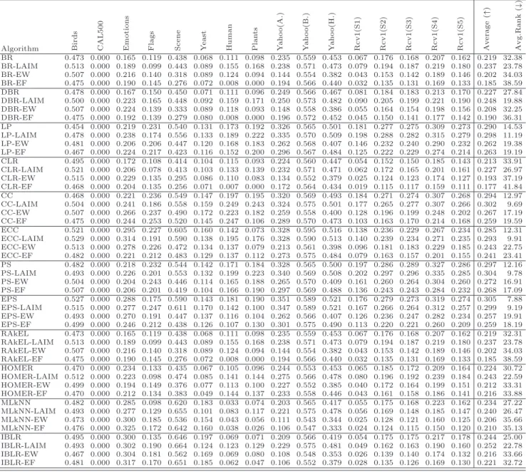
Algorithm Bir d s C A L 5 0 0 E m o ti o n s F la g s S c e n e Y e a st H u m a n P la n ts Y a h o o (A .) Y a h o o (B .) Y a h o o (H .) R c v 1 (S 1 ) R c v 1 (S 2 ) R c v 1 (S 3 ) R c v 1 (S 4 ) R c v 1 (S 5 ) A v e ra g e ( ↑ ) A v g .R a n k ( ↓ ) BR 0.473 0.000 0.165 0.119 0.438 0.068 0.111 0.098 0.235 0.559 0.453 0.067 0.176 0.168 0.207 0.162 0.219 32.38 BR-LAIM 0.513 0.000 0.189 0.099 0.443 0.089 0.155 0.168 0.238 0.571 0.473 0.079 0.194 0.187 0.219 0.180 0.237 23.78 BR-EW 0.507 0.000 0.216 0.140 0.318 0.089 0.124 0.094 0.144 0.554 0.382 0.043 0.153 0.142 0.189 0.146 0.202 34.03 BR-EF 0.475 0.000 0.190 0.145 0.276 0.072 0.008 0.000 0.194 0.566 0.440 0.032 0.135 0.131 0.169 0.133 0.185 38.59 DBR 0.478 0.000 0.167 0.150 0.450 0.071 0.111 0.096 0.249 0.566 0.467 0.081 0.184 0.183 0.213 0.170 0.227 27.84 DBR-LAIM 0.500 0.000 0.223 0.165 0.448 0.092 0.159 0.171 0.250 0.573 0.482 0.090 0.205 0.199 0.221 0.190 0.248 19.88 DBR-EW 0.507 0.000 0.224 0.139 0.333 0.089 0.118 0.093 0.148 0.558 0.386 0.055 0.164 0.154 0.198 0.156 0.208 32.25 DBR-EF 0.475 0.000 0.192 0.139 0.279 0.080 0.008 0.000 0.196 0.572 0.452 0.045 0.150 0.141 0.177 0.142 0.190 36.31 LP 0.454 0.000 0.219 0.231 0.540 0.131 0.173 0.192 0.326 0.565 0.501 0.181 0.277 0.275 0.309 0.273 0.290 14.53 LP-LAIM 0.478 0.000 0.238 0.174 0.556 0.133 0.189 0.222 0.335 0.570 0.509 0.198 0.288 0.282 0.315 0.279 0.298 11.19 LP-EW 0.481 0.000 0.206 0.206 0.447 0.120 0.168 0.183 0.262 0.568 0.407 0.146 0.232 0.240 0.290 0.232 0.262 19.38 LP-EF 0.467 0.000 0.224 0.217 0.423 0.116 0.152 0.200 0.296 0.567 0.484 0.125 0.222 0.229 0.274 0.214 0.263 19.19 CLR 0.495 0.000 0.172 0.108 0.414 0.104 0.115 0.093 0.224 0.560 0.447 0.054 0.152 0.150 0.185 0.143 0.213 33.91 CLR-LAIM 0.521 0.000 0.206 0.078 0.413 0.103 0.133 0.139 0.232 0.571 0.471 0.062 0.172 0.165 0.201 0.161 0.227 26.97 CLR-EW 0.515 0.000 0.229 0.135 0.295 0.086 0.110 0.083 0.134 0.552 0.379 0.025 0.124 0.123 0.174 0.127 0.193 37.19 CLR-EF 0.468 0.000 0.204 0.135 0.256 0.071 0.007 0.000 0.172 0.564 0.434 0.019 0.115 0.117 0.159 0.111 0.177 41.84 CC 0.468 0.000 0.221 0.236 0.549 0.147 0.197 0.195 0.320 0.569 0.493 0.184 0.271 0.274 0.307 0.268 0.294 12.97 CC-LAIM 0.504 0.000 0.241 0.186 0.558 0.159 0.249 0.243 0.324 0.575 0.501 0.177 0.265 0.277 0.307 0.266 0.302 9.69 CC-EW 0.507 0.000 0.266 0.237 0.490 0.172 0.223 0.182 0.259 0.558 0.400 0.128 0.196 0.199 0.248 0.202 0.267 17.19 CC-EF 0.475 0.000 0.244 0.253 0.520 0.145 0.247 0.106 0.289 0.570 0.473 0.103 0.163 0.170 0.214 0.168 0.259 19.59 ECC 0.521 0.000 0.295 0.227 0.605 0.160 0.142 0.073 0.328 0.595 0.516 0.138 0.236 0.229 0.267 0.234 0.285 12.31 ECC-LAIM 0.529 0.000 0.314 0.191 0.590 0.138 0.195 0.176 0.328 0.590 0.513 0.140 0.239 0.234 0.271 0.235 0.293 9.91 ECC-EW 0.513 0.000 0.278 0.226 0.472 0.134 0.137 0.079 0.213 0.561 0.398 0.096 0.181 0.183 0.229 0.185 0.243 22.75 ECC-EF 0.482 0.000 0.221 0.212 0.483 0.129 0.137 0.112 0.273 0.575 0.484 0.079 0.163 0.157 0.201 0.155 0.241 23.41 PS 0.482 0.000 0.218 0.232 0.544 0.142 0.171 0.184 0.328 0.565 0.500 0.197 0.286 0.289 0.327 0.286 0.297 12.16 PS-LAIM 0.493 0.000 0.226 0.201 0.553 0.132 0.199 0.223 0.340 0.569 0.508 0.202 0.297 0.296 0.335 0.285 0.304 9.78 PS-EW 0.504 0.000 0.204 0.243 0.446 0.114 0.165 0.188 0.265 0.570 0.409 0.161 0.260 0.264 0.304 0.260 0.272 16.91 PS-EF 0.507 0.000 0.206 0.201 0.419 0.104 0.166 0.190 0.297 0.569 0.488 0.136 0.243 0.243 0.284 0.232 0.268 17.09 EPS 0.527 0.000 0.288 0.175 0.590 0.143 0.181 0.190 0.351 0.589 0.521 0.176 0.279 0.273 0.319 0.274 0.305 7.88 EPS-LAIM 0.515 0.000 0.277 0.247 0.611 0.170 0.142 0.100 0.347 0.589 0.521 0.167 0.266 0.264 0.312 0.257 0.299 9.19 EPS-EW 0.493 0.000 0.270 0.191 0.447 0.137 0.116 0.104 0.262 0.566 0.407 0.126 0.236 0.247 0.282 0.234 0.257 19.91 EPS-EF 0.499 0.000 0.246 0.212 0.438 0.126 0.107 0.130 0.301 0.575 0.490 0.113 0.220 0.221 0.260 0.209 0.259 18.19 RAkEL 0.473 0.000 0.165 0.119 0.438 0.068 0.111 0.098 0.235 0.559 0.453 0.067 0.176 0.168 0.207 0.162 0.219 32.31 RAkEL-LAIM 0.513 0.000 0.189 0.099 0.443 0.089 0.155 0.168 0.238 0.571 0.473 0.079 0.194 0.187 0.219 0.180 0.237 23.78 RAkEL-EW 0.507 0.000 0.216 0.140 0.318 0.089 0.124 0.094 0.144 0.554 0.382 0.043 0.153 0.142 0.189 0.146 0.202 34.03 RAkEL-EF 0.475 0.000 0.190 0.145 0.276 0.072 0.008 0.000 0.194 0.566 0.440 0.032 0.135 0.131 0.169 0.133 0.185 38.59 HOMER 0.470 0.000 0.234 0.133 0.435 0.067 0.105 0.096 0.244 0.553 0.453 0.065 0.185 0.172 0.209 0.164 0.224 30.72 HOMER-LAIM 0.512 0.000 0.223 0.098 0.474 0.085 0.141 0.144 0.275 0.566 0.478 0.080 0.196 0.192 0.239 0.184 0.243 22.59 HOMER-EW 0.499 0.000 0.194 0.149 0.376 0.077 0.113 0.100 0.227 0.552 0.385 0.040 0.172 0.164 0.199 0.151 0.212 33.31 HOMER-EF 0.470 0.000 0.212 0.134 0.383 0.049 0.144 0.137 0.233 0.558 0.446 0.043 0.161 0.158 0.186 0.141 0.216 33.88 MLkNN 0.482 0.000 0.285 0.098 0.620 0.183 0.033 0.074 0.203 0.565 0.417 0.055 0.175 0.168 0.223 0.162 0.234 27.22 MLkNN-LAIM 0.493 0.000 0.277 0.129 0.655 0.101 0.083 0.117 0.221 0.575 0.478 0.056 0.169 0.148 0.185 0.147 0.240 26.47 MLkNN-EW 0.473 0.000 0.300 0.185 0.536 0.154 0.043 0.056 0.111 0.543 0.344 0.025 0.128 0.121 0.160 0.125 0.206 35.66 MLkNN-EF 0.476 0.000 0.325 0.172 0.642 0.160 0.038 0.026 0.106 0.547 0.333 0.024 0.124 0.115 0.150 0.120 0.210 35.13 IBLR 0.495 0.000 0.300 0.135 0.646 0.197 0.069 0.071 0.209 0.566 0.419 0.054 0.175 0.175 0.217 0.178 0.244 25.00 IBLR-LAIM 0.493 0.000 0.302 0.190 0.664 0.124 0.123 0.129 0.229 0.575 0.481 0.049 0.162 0.163 0.190 0.160 0.252 22.78 IBLR-EW 0.467 0.000 0.304 0.181 0.562 0.169 0.069 0.080 0.108 0.548 0.353 0.026 0.139 0.140 0.174 0.132 0.216 33.66 IBLR-EF 0.481 0.000 0.317 0.170 0.651 0.185 0.062 0.047 0.106 0.552 0.379 0.028 0.135 0.126 0.169 0.130 0.221 32.72

Table 9: Results obtained for subset accuracy (↑)

improved on 4 datasets for 11 algorithms, 4 other datasets for 10 algorithms, and 5 other datasets for 9 algorithms. However, only the discretization of the yeast dataset was found not to be improved by a majority of multi-label classifiers as measured by the Hamming loss. Similarly, Table 8 shows the

results obtained for ranking loss. LAIM discretization improves the average ranking values on 7 of the 12 classifiers. However, performance was worse on ECC, MLkNN, and IBLR. On the other hand, unsupervised discretizers obtained much worse performance both on Hamming loss and ranking loss.

Table 9 shows the results obtained for the subset accuracy. This is a very strict evaluation measure as it requires the predicted set of labels to be an exact match of the true set of labels (notice that for CAL500, there is any algorithm capable of predicting the whole labelset correctly). Results show that LAIM discretization improves the average ranking values for 11 out of 12 algorithms. Specifically, 4 algorithms (BR, DBR, LP, RAkEL) achieve better performance on discretized data in 14 out of 16 datasets, HOMER on 13 datasets, and 2 algorithms (CLR, PS) on 12 datasets. However, EPS is the only algorithm whose performance on discretized data was worse as measured by the subset accuracy. On the other hand, from the point of view of datasets, subset accuracy was improved on 3 datasets for 11 algorithms, 3 other datasets for 10 algorithms, and 5 other datasets for 9 algorithms. However, only the discretization of the flags dataset was found not to be improved by a majority of multi-label classifiers as measured by the subset accuracy. Again, unsupervised discretization showed to achieve much worse results. In summary, these results show that there is a majority of datasets which are improved after LAIM discretization for a majority of algorithms.

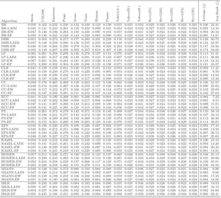
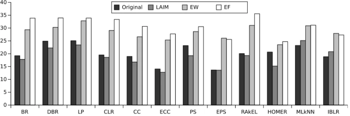
Moreover, we show all the rank results for all metrics gathered in Ta-ble 10. Besides, a meta-ranking of algorithms (the rank of the ranks) was built following the philosophy of the Friedman test described above. This way, we can evaluate which algorithm has best overall performance in most of the metrics, since there is any method that performs best for all the met-rics. In this case, the algorithm with the best value in one metric was given a rank of 1 for that metric, the algorithm with the next best value had the rank of 2, and so on. Finally, the average ranks of each algorithm in all metrics were calculated. Results are depicted in Figures 1 and 2, which illustrate the average rank and meta-rank of the algorithms with and without LAIM discretization. As can be observed, LAIM data discretization improves the average rank and meta-rank in 10 of the 12 algorithms whereas unsupervised methods obtain much worse ranks. It is worthy to mention the significant performance improvement on the HOMER and PS algorithms after data dis-cretization. On the other hand, only MLkNN and IBLR get worse ranks. Particularly, MLkNN and IBLR are two instance-based algorithms, and the deterioration of results may be due to the fact they are very influenced by

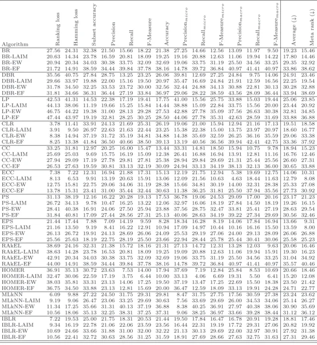
Algorithm Ra n k in g lo ss H a m m in g lo ss S u b se t a c c u ra c y P re c is io n R e c a ll F -M e a su re A c c u ra c y P re c is io nm i c r o R e c a llm i c r o F -M e a su re m i c r o P re c is io nm a c r o R e c a llm a c r o F -M e a su re m a c r o A v e ra g e ( ↓ ) M e ta ra n k ( ↓ ) BR 27.56 24.31 32.38 21.50 15.66 18.22 21.38 27.25 14.66 12.56 13.09 11.97 9.50 19.23 15.46 BR-LAIM 20.63 14.34 23.78 16.59 20.81 18.09 19.25 19.16 20.88 12.63 11.06 19.94 14.22 17.80 14.46 BR-EW 20.94 20.34 34.03 30.38 33.75 32.09 32.69 19.06 33.75 31.19 25.50 34.56 33.25 29.35 32.92 BR-EF 21.72 14.91 38.59 34.44 39.84 37.78 38.16 14.78 39.72 36.84 40.97 41.41 40.97 33.86 38.62 DBR 35.56 40.75 27.84 28.75 13.25 23.25 26.06 39.81 12.69 27.25 24.84 9.75 14.06 24.91 23.46 DBR-LAIM 29.66 33.97 19.88 22.00 15.16 19.50 20.97 35.47 16.69 24.84 21.91 12.59 16.56 22.25 19.54 DBR-EW 31.78 34.50 32.25 33.53 23.72 30.00 32.56 32.44 24.88 34.13 30.88 22.81 30.13 30.28 32.88 DBR-EF 31.81 34.66 36.31 36.44 27.19 33.84 36.97 29.06 28.22 38.59 43.56 28.09 36.44 33.94 38.69 LP 42.53 41.31 14.53 22.38 17.19 19.41 17.75 41.00 15.56 25.75 33.88 15.03 19.44 25.06 23.85 LP-LAIM 44.13 38.06 11.19 19.66 15.25 15.84 14.44 38.88 15.09 22.84 33.75 15.56 20.00 23.44 20.92 LP-EW 46.75 44.22 19.38 31.00 28.13 29.28 27.53 42.88 27.78 35.09 37.56 26.63 30.38 32.81 34.85 LP-EF 47.44 43.97 19.19 32.81 28.25 30.25 28.50 44.06 27.78 35.31 42.63 28.59 31.69 33.88 36.88 CLR 3.78 11.41 33.91 24.13 21.69 25.31 26.19 19.06 21.00 15.94 12.94 21.16 17.13 19.51 18.58 CLR-LAIM 3.91 9.50 26.97 22.63 21.63 22.44 23.25 15.38 22.38 15.00 13.75 23.97 20.97 18.60 16.77 CLR-EW 8.38 14.94 37.19 31.72 35.19 34.81 34.88 14.38 35.69 32.59 26.25 36.16 35.59 29.06 33.38 CLR-EF 8.25 13.38 41.84 36.50 40.66 38.50 39.13 13.19 40.56 36.56 39.94 42.41 42.75 33.36 37.92 CC 33.25 31.81 12.97 20.25 16.00 15.47 13.44 33.31 14.81 18.50 15.94 10.75 9.78 18.94 15.23 CC-LAIM 25.69 25.03 9.69 15.75 16.19 15.09 12.38 26.41 16.88 16.94 13.91 12.81 11.16 16.76 12.46 CC-EW 27.94 29.09 17.19 27.78 29.81 27.81 25.38 28.94 29.84 29.69 21.31 25.44 25.56 26.60 27.31 CC-EF 26.53 27.63 19.59 30.81 33.13 32.19 30.09 24.94 33.13 34.19 38.13 32.13 36.00 30.65 33.88 ECC 7.38 7.22 12.31 16.94 21.88 17.31 15.13 12.19 21.75 12.94 5.38 19.69 12.75 14.06 10.31 ECC-LAIM 8.13 6.53 9.91 13.19 20.63 15.91 13.06 12.09 21.56 10.63 4.63 18.44 11.63 12.79 8.08 ECC-EW 12.75 15.81 22.75 29.06 34.06 31.19 28.38 15.66 34.81 30.19 14.00 32.31 28.38 25.33 27.08 ECC-EF 13.78 15.31 23.41 31.00 35.44 32.44 30.63 11.38 36.25 31.81 25.50 37.94 35.56 27.73 30.92 PS 31.13 38.19 12.16 16.22 20.28 19.13 17.53 36.78 19.06 24.53 29.09 17.00 20.16 23.17 21.23 PS-LAIM 26.72 34.13 9.78 10.47 16.25 13.22 12.06 32.97 16.06 18.19 27.84 14.50 18.19 19.26 16.15 PS-EW 28.41 40.38 16.91 24.06 27.50 25.94 23.88 37.56 28.75 32.47 33.81 25.41 27.19 28.63 29.54 PS-EF 31.84 40.81 17.09 27.44 28.56 27.31 25.13 40.06 28.63 34.19 39.22 27.34 29.69 30.56 32.46 EPS 21.44 17.44 7.88 7.09 14.19 9.59 8.28 18.34 16.28 8.19 14.06 17.84 16.94 13.66 9.31 EPS-LAIM 21.16 13.50 9.19 8.41 16.22 12.91 10.94 17.09 14.97 10.44 10.16 16.16 15.50 13.59 8.00 EPS-EW 26.13 26.72 19.91 24.13 28.69 26.06 24.09 25.53 29.19 27.06 24.00 29.13 28.09 26.06 26.88 EPS-EF 25.56 25.63 18.19 22.75 28.19 25.50 23.66 22.94 28.44 25.78 25.44 30.41 30.06 25.58 25.23 RAkEL 38.69 24.16 32.31 21.38 15.72 18.16 21.31 27.13 14.72 12.31 13.28 12.03 9.63 20.06 16.46 RAkEL-LAIM 38.63 14.28 23.78 16.53 20.81 18.09 19.25 19.09 20.88 12.63 11.06 19.94 15.91 19.30 16.23 RAkEL-EW 42.91 20.34 34.03 30.38 33.75 32.09 32.69 19.06 33.75 31.19 25.50 34.56 33.25 31.04 34.92 RAkEL-EF 44.00 14.91 38.59 34.44 39.84 37.78 38.16 14.78 39.72 36.84 40.97 41.41 40.97 35.57 40.46 HOMER 36.91 35.13 30.72 23.63 7.53 14.00 17.94 37.69 7.19 12.84 25.84 8.53 10.69 20.66 18.46 HOMER-LAIM 32.47 30.06 22.59 17.19 3.75 6.44 10.00 33.13 4.06 6.69 19.31 5.50 6.41 15.20 12.08 HOMER-EW 38.03 35.81 33.31 23.13 14.06 17.25 19.50 37.19 13.47 17.25 22.69 15.50 18.38 23.50 21.42 HOMER-EF 36.75 34.50 33.88 23.13 12.81 15.69 20.00 36.47 12.59 18.09 33.13 19.91 24.28 24.71 22.77 MLkNN 6.09 9.88 27.22 24.50 31.75 29.31 29.81 8.47 31.75 27.75 17.56 30.59 27.38 23.24 23.62 MLkNN-LAIM 9.19 9.06 26.47 23.06 33.25 29.69 30.63 7.56 33.69 29.69 26.00 34.53 34.06 25.14 26.27 MLkNN-EW 11.34 17.25 35.66 31.31 40.13 37.19 36.88 8.38 40.25 36.91 27.97 40.38 38.06 30.90 35.69 MLkNN-EF 10.56 18.06 35.13 32.25 38.31 37.25 37.31 9.06 38.25 36.97 33.66 39.28 38.44 31.12 36.12 IBLR 7.22 19.53 25.00 21.75 18.31 20.53 21.44 19.50 17.84 16.47 16.78 20.91 19.28 18.81 17.46 IBLR-LAIM 9.34 16.19 22.78 21.06 22.06 23.59 23.56 16.44 22.31 19.19 17.72 29.31 27.06 20.82 19.92 IBLR-EW 10.69 24.66 33.66 31.88 31.00 32.00 32.22 21.13 30.13 29.69 22.00 32.97 30.91 27.92 31.38 IBLR-EF 10.56 22.41 32.72 30.63 28.56 31.25 31.59 18.91 27.69 28.66 27.63 32.75 31.63 27.31 29.46

Table 10: Average rankings for all metrics and algorithms (↓)

continuous features and discretization affects the actual calculation of dis-tances.

BR DBR LP CLR CC ECC PS EPS RAkEL HOMER MLkNN IBLR 0 5 10 15 20 25 30 35 40 Original LAIM EW EF

Figure 1: Average rankings of algorithms with and without discretization (↓)

BR DBR LP CLR CC ECC PS EPS RAkEL HOMER MLkNN IBLR 0 5 10 15 20 25 30 35 40 45 Original LAIM EW EF

Figure 2: Meta ranks of algorithms with and without discretization (↓)

5.1. Statistical analysis

In order to determine whether preprocessing data with multi-label LAIM discretization is able to significantly improve performance, the Wilcoxon [54] test was carried out for each couple of algorithms considering the values in Table 10. Wilcoxon rank sum test is a non-parametric one recommended in Demˇsar’s study [15], which allows us to address whether there are significant differences between the performance values obtained with and without the LAIM discretization. To do this, the null hypothesis of this test maintains that there are no significant differences between the performance values, while the alternative hypothesis assures that there are. Table 11 shows the sum of ranks, the p-values and the statistical confidence.

From the p-value column, it can be concluded that there are significant differences at a 90% level of confidence (p-value ≤ 0.1) in the case of CC. There are also significant differences at a 95% level of confidence (p-value ≤

LAIM discret. vs. R+ R− _{Exactp-value Asymptoticp-value Confidence} BR 60.0 31.0 ≥0.2 0.2945 -DBR 76.0 15.0 0.0327 0.0302 95% LP 79.0 12.0 0.0171 0.0174 95% CLR 61.0 30.0 ≥0.2 0.2634 -CC 71.0 20.0 0.0803 0.0667 90% ECC 86.5 4.5 0.0020 0.0031 99% PS 91.0 0.0 2.44E-4 0.0039 99% EPS 46.0 45.0 ≥0.2 0.9437 -RAkEL 54.0 37.0 ≥0.2 0.5257 -HOMER 91.0 0.0 2.44E-4 0.0013 99% MLkNN 16.5 74.5 ≥0.2 1 -IBLR 22.5 68.5 ≥0.2 1

-Table 11: Algorithms comparison: results obtained by the Wilcoxon test

0.05) in the case of DBR and LP, and even there are significant differences at a 99% level of confidence (p-value ≤ 0.01) in the case of ECC, PS and HOMER. This means that the discretization method proposed in this paper effectively improves classification performance for the datasets and metrics tested with DBR, CC, ECC, LP, PS and HOMER. In BR, CLR and RAkEL there are not significant differences, but the sum of ranks is still higher for discretization. On the other hand, in the case of instance-based algorithms, MLkNN and IBLR, the sum of ranks is quite higher without discretization. Therefore, it is not recommendable to perform data discretization prior the execution of these two instance-based algorithms.

Finally, one more test has been carried out, in this case in order to eval-uate whether discretization improves particular performance metrics. The Wilcoxon test was carried out for each metric considering values obtained with and without discretization. Table 12 summarizes the results of the test performed. In the light of the results we can conclude that there are signifi-cant differences in 5 of the 13 metric evaluated. Results obtained for example-based accuracy significantly improve with LAIM discretization with a 95% level of confidence and finally, Hamming loss, subset accuracy, example-based precision, and precisionmicro results are improved with discretization at a 99%

level of significance. In the case of ranking loss, example-based F-Mreasure, F-measuremicro, and precisionmacro there are not significant differences, but

the sum of ranks is higher with discretization.

It is important to highlight that discretization statistically improved multi-label classification considering the Haming loss and the subset accuracy. The

Metric R+ R− _{Exactp-value Asymptoticp-value Confidence}

Hamming Loss 78.0 0.0 4.88E-4 0.0017 99% Ranking Loss 54.0 24.0 ≥0.2 0.2240 -Subset Accuracy 76.0 2.0 0.0014 0.0032 99% Precision 76.0 2.0 0.0014 0.0032 99% Recall 29.0 49.0 ≥0.2 1 -F-Measure 59.5 18.5 0.1196 0.0961 -Accuracy 64.5 13.5 0.0473 0.0374 95% Precisionmicro 78.0 0.0 4.88E-4 0.0019 99% Recallmicro 21.0 57.0 ≥0.2 1 -F-measuremicro 55.0 23.0 ≥0.2 0.1955 -Precisionmacro 59.0 19.0 0.1294 0.1078 -Recallmacro 18.0 60.0 ≥0.2 1 -F-measuremacro 19.0 59.0 ≥0.2 1 -Meta-rank 65.0 13.0 0.0424 0.0376 95% Table 12: Metrics comparison: results obtained by the Wilcoxon test

former is the most frequently reported whereas the latter is considered overly stringent [14] since making a mistake on a single label is punished hardly. Therefore, improving both metrics simultaneously is worth to mention.

5.2. Space and time complexity

Space and time complexity are essential for scaling algorithms to large-scale and big data. The LAIM time complexity for discretizing an attribute is O(m log m), where m is the number of distinct (unique) values of the attribute. The LAIM space complexity is O(n·q), where n is the number of intervals and qis the number of labels. Therefore, it can easily scale to large problems. Moreover, discretization of multiple attributes can be parallelized using CPU threads or GPUs [7].

Table 13 shows the discretization time for the datasets. Considering their complexity as measured by the number of instances and attributes (see Ta-ble 5), the LAIM discretization is fast and scalaTa-ble, having a maximum run-time lower than 3 seconds for the Rcv1 datasets, which comprise a larger number of instances, attributes and labels. Thus, given LAIM complexities it is not expected to have space or time problems when addressing high-dimensional data from similar researches [44].

Dataset Time (ms) Dataset Time (ms) Flags 52 Yahoo(A.) 967 Emotions 264 Yahoo(H.) 1129 Birds 419 Yahoo(B.) 1275 Yeast 1912 Rcv1(S1) 2911 Scene 2570 Rcv1(S2) 2792 Plant 706 Rcv1(S3) 2605 CAL500 743 Rcv1(S4) 2422 Human 1394 Rcv1(S5) 2671

Table 13: Discretization runtime (milliseconds)

6. Conclusion

In this paper we presented a Label-Attribute Interdependence Maximiza-tion (LAIM) discretizaMaximiza-tion algorithm for multi-label data which extended the CAIM principles. Its flexible representation of a multi-label quanta matrix allowed to adapt the discretization process to data instances having multi-ple labels. The experimental study analyzed the performance differences of 12 classification algorithms with and without discretization on 13 multi-label metrics. Experimental results showed the better performance with discretiza-tion on 10 of the 12 algorithms by means of the average ranks of the classifiers. Specifically, HOMER, PS and ECC improved their performance significantly as compared with the results without discretization. On the other hand, instance-based methods as MLkNN and IBLR showed worse performance af-ter discretization. Unsupervised discretizers were also analyzed showing to achieve significantly worse performance. With regards of the performance metrics, multi-label discretization demonstrated to improve the Hamming loss, the subset accuracy, the example-based precision, the accuracy, and the precisionmicro. Results were validated through non-parametric statistical

analysis which evidenced the performance improvements on each of the al-gorithms and metrics. The good results obtained indicate that multi-label discretization is an open challenge demanding further research.

Acknowledgements

This research was supported by the Spanish Ministry of Economy and Competitiveness, project TIN2014-55252-P, and by FEDER funds. This re-search was also supported by the Spanish Ministry of Education under FPU grants AP2010-0041 and AP2010-0042.

References

[1] J. L. ´Avila, E. L. Gibaja, A. Zafra, and S. Ventura. A Gene Expres-sion Programming Algorithm for Multi-Label Classification. Journal of Multiple-Valued Logic and Soft Computing, 17:183–206, 2011.

[2] C. Bielza, G. Li, and P. Larra˜naga. Multi-dimensional classification with Bayesian networks. Int. J. Approx. Reasoning, 52(6):705–727, 2011. [3] M. Boutell, J. Luo, X. Shen, and C. Brown. Learning multi-label scene

classification. Pattern Recognition, 37(9):1757–1771, 2004.

[4] F. Briggs, R. Raich, K. Eftaxias, Z. Lei, , and Y. Huang. The ninth annual MLSP competition: Overview. In Proceedings of the IEEE In-ternational Workshop on Machine Learning for Signal Processing, pages 1–2, 2013.

[5] K. Brinker, J. F¨urnkranz, and E. H¨ullermeier. A Unified Model for Mul-tilabel Classification and Ranking. In Proceeding of the 17th European Conference on Artificial Intelligence, pages 489–493, 2006.

[6] A. Cano, D. T. Nguyen, S. Ventura, and K. J. Cios. ur-CAIM: improved CAIM discretization for unbalanced and balanced data.Soft Computing, In press, 2015.

[7] A. Cano, S. Ventura, and K. Cios. Scalable CAIM discretization on multiple GPUs using concurrent kernels. Journal of Supercomputing, 69(1):273–292, 2014.

[8] W. Cheng and E. H¨ullermeier. Combining instance-based learning and logistic regression for multilabel classification. Machine Learning, 76(2-3):211–225, 2009.

[9] T. Cheng-Jung, L. Chien-I, and Y. Wei-Pang. A discretization algorithm based on class-attribute contingency coefficient. Information Sciences, 178:714–731, 2008.

[10] B. S. Chlebus and S. H. Nguyen. On Finding Optimal Discretizations for Two Attributes. In Proceedings of the 1st Int. Conf. Rough Sets and Current Trends in Computing (RSCTC 98), pages 537–544, 1998.

[11] A. Clare and R. D. King. Knowledge Discovery in Multi-label Phenotype Data. Lecture Notes in Computer Science, 2168:42 – 53, 2001.

[12] K. Crammer and Y. Singer. A family of additive online algorithms for category ranking. Journal of Machine Learning Research, 3:1025–1058, 2003.

[13] C. De Sa, C. Soares, and A. Knobbe. Entropy-based discretization meth-ods for ranking data. Information Sciences, In press, 2015.

[14] K. Dembczynski, W. Waegeman, W. Cheng, and E. Hullermeier. Regret analysis for performance metrics in multi-label classification: The case of hamming and subset zero-one loss. In Machine Learning and Knowl-edge Discovery in Databases (2010), volume 6321 LNCS, pages 280–295, 2010.

[15] J. Demˇsar. Statistical Comparisons of Classifiers over Multiple Data Sets. Journal of Machine Learning Research, 7:1–30, 2006.

[16] R. Duwairi and A. Kassawneh. A framework for predicting proteins 3D structures. In IEEE/ACS International Conference on Computer Systems and Applications (AICCSA ’08), pages 37 –44, 2008.

[17] A. Elisseeff and J. Weston. Kernel methods for Multi-labelled classifi-cation and Categorical regression problems. Advances in Neural Infor-mation Processing Systems, 14:681–687, 2001.

[18] U. M. Fayyad and K. B. Irani. Multi-Interval Discretization of Continuous-Valued Attributes for Classification Learning. In Proceed-ings of the 13th International Joint Conference on Artificial Intelligence, pages 1022–1029, 1993.

[19] S. Garc´ıa, A. Fern´andez, J. Luengo, and F. Herrera. Advanced non-parametric tests for multiple comparisons in the design of experiments in computational intelligence and data mining: Experimental analysis of power. Information Sciences, 180(10):2044–2064, 2010.

[20] S. Garc´ıa, J. Luengo, J. S´aez, V. L´opez, and F. Herrera. Survey of Discretization Techniques: Taxonomy and Empirical Analysis in Super-vised Learning. IEEE Transactions on Knowledge and Data Engineer-ing, 25(4):734–750, 2013.

[21] E. Gibaja and S. Ventura. Multi-label learning: a review of the state of the art and ongoing research. WIREs Data Mining Knowledge Discov-ery, 4(6):411–444, 2014.

[22] E. C. Gon¸calves, A. Plastino, and A. A. Freitas. A Genetic Algorithm for Optimizing the Label Ordering in Multi-Label Classifier Chains. In

International Conference on Tools with Artificial Intelligence (ICTAI), pages 469–476, 2013.

[23] M. Hassan, A. Karim, J.-B. Kim, and M. Jeon. CDIM: Document clus-tering by discrimination information maximization. Information Sci-ences, 316:87–106, 2015.

[24] K. Kawai and Y. Takahashi. Identification of the Dual Action Antihy-pertensive Drugs Using TFS-Based Support Vector Machines.Chem-Bio Informatics Journal, 4:44–51, 2009.

[25] R. Kerber. ChiMerge: Discretization of Numeric Attributes. In Pro-ceedings of the 10th National Conference on Artificial Intelligence, pages 123–128, 1992.

[26] S. Kotsiantis and D. Kanellopoulos. Discretization techniques: A recent survey. GESTS International Transactions on Computer Science and Engineering, 32(1):47–58, 2006.

[27] A. Krohn-Grimberghe, L. Drumond, C. Freudenthaler, and L. Schmidt-Thieme. Multi-relational matrix factorization using bayesian personal-ized ranking for social network data. In Proceedings of the 5th ACM International Conference on Web Search and Data Mining (WSDM), pages 173–182. ACM, 2012.

[28] L. A. Kurgan and K. J. Cios. CAIM Discretization Algorithm. IEEE Transactions on Knowledge and Data Engineering, 16(2):145–153, 2004. [29] J. Lee and D.-W. Kim. Memetic feature selection algorithm for

multi-label classification. Information Sciences, 293:80–96, 2015.

[30] S.-J. Lee, M.-T. Jone, and H.-L. Tsai. Constructing neural net-works for multiclass-discretization based on information entropy. IEEE Transactions on Systems, Man, and Cybernetics, Part B: Cybernetics, 29(3):445–453, 1999.

[31] D. D. Lewis, Y. Yang, T. G. Rose, and F. Li. RCV1: A New Bench-mark Collection for Text Categorization Research. Journal of Machine Learning Research, 5:361–397, 2004.

[32] H. Liu and R. Setiono. Feature selection via discretization. IEEE Trans-actions on Knowledge and Data Engineering, 9:642–645, 1997.

[33] G. Madjarov, D. Kocev, D. Gjorgjevikj, and S. Dˇzeroski. An extensive experimental comparison of methods for multi-label learning. Pattern Recognition, 45(9):3084–3104, 2012.

[34] A. K. McCallum. Multi-label text classification with a mixture model trained by EM. In AAAI 99 Workshop on Text Learning, 1999.

[35] E. Montanes, R. Senge, J. Barranquero, J. R. Quevedo, J. J. del Coz, and E. Hullermeier. Dependent binary relevance models for multi-label classification. Pattern Recognition, 47(3):1494–1508, 2014.

[36] P. Nardiello, F. Sebastiani, and A. Sperduti. Discretizing Continuous Attributes in AdaBoost for Text Categorization. In Advances in Infor-mation Retrieval, volume 2633 of Lecture Notes in Computer Science, pages 320–334. 2003.

[37] M. J. Pazzani. An Iterative Improvement Approach for the Discretiza-tion of Numeric Attributes in Bayesian Classifiers. InProceedings of the 1st International Conference on Knowledge Discovery and Data Mining, pages 228–233, 1995.

[38] J. Pestian, C. Brew, P. Matykiewicz, D. Hovermale, N. Johnson, K. Co-hen, and W. Duch. A shared task involving multi-label classification of clinical free text. In Proceedings of ACL BioNLP, pages 97–104, 2007. [39] R. Rak, L. Kurgan, and M. Reformat. A tree-projection-based algorithm

for multi-label recurrent-item associative-classification rule generation.

Data & Knowledge Engineering, 64(1):171–197, 2008.

[40] J. Read. A Pruned Problem Transformation Method for Multi-label Classification. In Proceedings of the NZ Computer Science Research Student Conference, pages 143–150, 2008.