Title: Machine Learning Prediction of NanoparticleIn Vitro Toxicity: A Comparative Study of Classifiers and
Ensemble-Classifiers using the Copeland Index
Authors: Irini Furxhi, Finbarr Murphy, Martin Mullins, Craig A. Poland
PII: S0378-4274(19)30147-X
DOI: https://doi.org/10.1016/j.toxlet.2019.05.016
Reference: TOXLET 10491
To appear in: Toxicology Letters Received date: 23 January 2019 Revised date: 12 April 2019 Accepted date: 13 May 2019
Please cite this article as: Furxhi I, Murphy F, Mullins M, Poland CA, Machine Learning Prediction of Nanoparticle In Vitro Toxicity: A Comparative Study of Classifiers and Ensemble-Classifiers using the Copeland Index, Toxicology Letters (2019), https://doi.org/10.1016/j.toxlet.2019.05.016
This is a PDF file of an unedited manuscript that has been accepted for publication. As a service to our customers we are providing this early version of the manuscript. The manuscript will undergo copyediting, typesetting, and review of the resulting proof before it is published in its final form. Please note that during the production process errors may be discovered which could affect the content, and all legal disclaimers that apply to the journal pertain.
Machine Learning Prediction of Nanoparticle In Vitro Toxicity: A Comparative Study of Classifiers and Ensemble-Classifiers using the Copeland Index.
Irini Furxhi a, Finbarr Murphy*a, Martin Mullinsa, Craig A. Polandb
aDept. of Accounting and Finance, Kemmy Business School, University of Limerick, Ireland. V94PH93
b Centre for Inflammation Research, Queen’s Medical Research Institute, 47 Little France Crescent, University of Edinburgh, Scotland, EH16 4TJ
*Corresponding author [email protected]. Tel: +353 85 106 9771 *[email protected]. Tel: +353 86 108 8137 [email protected]. Tel: +353 85 108 6426 [email protected]. Tel: +44 131 242 6661 Graphical abstract
ACCEPTED MANUSCRIPT
Highlights
Random Forest (RF) and Neural Network (NN) have the best performance compared to the other base classifiers.
Ensemble classifiers have a better robust capability in predicting the toxicity of NP based on physicochemical properties, quantum-mechanical, toxicological attributes and in vitro experimental conditions compared to base classifiers.
RF and NN combined with another base classifier have not the best performance. Combining lower rank classifiers can help to catch the outliers.
Copeland Index based on datasets, validation processes and performance metrics can be used to rank base and ensemble classifiers.
RF, Bayesian Network (BN) and ensemble classifiers show high performances with missing values while NN did not.
Abstract
Nano-Particles (NPs) are well established as important components across a broad range of products from cosmetics to electronics. Their utilization is increasing with their significant economic and societal potential yet to be fully realized. Inroads have been made in our understanding of the risks posed to human health and the environment by NPs but this area will require continuous research and monitoring. In recent years Machine Learning (ML) techniques have exploited large datasets and computation power to create breakthroughs in diverse fields from facial recognition to genomics. More recently, ML techniques have been applied to nanotoxicology with very encouraging results. In this study, categories of ML classifiers (rules, trees, lazy, functions and bayes) were compared using datasets from the Safe and Sustainable Nanotechnology (S2NANO) database to investigate their performance in predicting NPs in vitro toxicity. Physicochemical properties, toxicological and quantum-mechanical attributes and in vitro experimental conditions were used as input variables to predict the toxicity of NPs based on cell viability. Voting, an ensemble meta-classifier, was
used to combine base models to optimize the classification prediction of toxicity. To facilitate inter-comparison, a Copeland Index was applied that ranks the classifiers according to their performance and suggested the optimal classifier. Neural Network (NN) and Random forest (RF) showed the best performance in the majority of the datasets used in this study. However, the combination of classifiers demonstrated an improved prediction resulting meta-classifier to have higher indices. This proposed Copeland Index can now be used by researchers to identify and clearly prioritize classifiers in order to achieve more accurate classification predictions for NP toxicity for a given dataset.
Abbreviations
RF Random Forest SENS Sensitivity
NN Neural Network SPEC Specificity
BN Bayesian Network ACC Balanced Accuracy
SMO Sequential Minimal Optimization F1 F1-score
LR Linear Regression DP Discriminant Power
IBk Instance Based k-nearest neighbour INT Internal
DT Decision Table EXT External
LWL Locally Weighted Learning REL Reliability GLM Generalized Linear Model BD Balanced Dataset SVM Support Vector Machines ID Imbalanced Dataset kNN k-Nearest Neighbour NP Nano-Particle SIR (Support Vector Machine-Instance Based k-nearest neighbour-Random Forest) DIR (Decision Table-Instance Based k-nearest neighbour-Random Forest)
NIR (Neural Network-Instance Based k-nearest neighbour-Random Forest)
LIR (Lazy-Instance Based k-nearest neighbour-Random Forest) BIR (Bayes-Instance Based k-nearest neighbour-Random Forest)
Keywords: Machine Learning; Voting; Nanotoxicity; Nanoparticles; Copeland Index;
1 Introduction
Nano-Particles (NPs) a broad classification of particulates, differing in various
physiochemical attributes such as shape, surface area, composition and other properties yet all sitting within the defined nano-range of 1-100nm. Such physicochemical attributes can imbue NPs with enhanced properties and as such, they are produced for a wide variety of
applications for example cosmetics, drugs and medications, biomedical devices, microelectronics and energy harvesting. Despite their increasing application across
innumerable product lines and their numerous benefits, further research on their hazardous effects on humans and the environment is required to ensure safety and sustainability [2, 3]. Nanotoxicology is a branch of toxicology that analyses the toxicity of NPs. Such analysis is necessary to identify their potential harmful effects on humans, animals or the environment. In vivo animal toxicity tests are constrained by time, ethical considerations and financial burdens [4]. Powerful techniques such as high throughput screening play an
important role for the hazard determination of NPs [5, 6]. Those methods are often expensive and time-consuming, especially in the case of NPs where a wide range of different NP’s physicochemical properties may alter the final hazard evaluation [2, 7-9]. Additional
attributes important for the manifestation of the toxicity are experimental conditions such as duration of exposure, exposure dose, and the cell line exposed to the substance [10-13].
Risk assessment and regulation have been a challenge due to insufficient and
inadequate information concerning the hazard and exposure assessment [14-16]. The field of nanotoxicology is interested in the performance and flexibility of computational methods that can predict the toxicity of NPs covering the diversity of chemical and biological behaviours along with exposure experimental conditions. Computational methods aim to complement in vitro and in vivo toxicity tests by minimizing the need for animal testing, reducing the cost and time of toxicity tests, and improving toxicity prediction and safety assessment. Machine Learning (ML) tools are gaining popularity in predicting toxicity due to their ability to combine a variety of information sources such as physicochemical properties and exposure conditions to predict endpoints of interest [17-24]. ML is, at its most basic, the practice of using algorithms to parse data, learn from that data and then to make predictions about an endpoint of interest.
Classification is a ML technique that assigns variables in a collection to predict
outcomes. The most popular classifiers in predicting the toxicity of NPs range from artificial Neural Networks (NN) [1, 10], Bayesian Networks (BN) [12, 25-27], Quantitative Structure Activity Relationships (QSARs aka nano-QSARs) [18, 28, 29], Linear Regression (LR), Random Forest (RF) and Support Vector Machines (SVM) [14, 30, 31]. Recently, integrated approaches (ensemble classifiers) are used to merge results from individual classifiers (base) in order to optimize the predictions [32-37]. Voting is a comprehensive ensemble learning method that collect votes from multiple base classifiers to predict the outcome via a voting mechanism to obtain a better predictive performance [38, 39].
The toxicity of NPs is an increasingly important research area worldwide in recent times [3] through a wish to ensure the sustainability of this new technology and not repeat mistakes of the past [40]. ML has been an essential tool for predicting the toxicity surrogating
the relationship between input and output. Classifiers are one of the most common ML tools exploiting experimental data such as physicochemical properties, quantum-mechanical attributes and toxicological outputs for nanotoxicity prediction [13, 28, 41]. Despite the wide variety and selection of classifiers and modelling approaches, no optimal classifier can be identified so far [32, 42]. Instead the predictability of the classifier depends on the dataset characteristics (missing values, training size, input variables) or the methods used to assess classifier performance [32].
The objective of this study is to:
a) apply classification models investigating how appropriate they are for each analysis scenario (datasets, validation, performance metrics),
b) generate integrated classifiers to increase the overall performance in all scenarios, c) develop an index capable of prioritizing the most appropriate classifier for NPs toxicity and
d) investigate the performance of base and ensemble classifiers with different ratios of missing data.
We demonstrate the efficacy of base and ensemble classifiers using different datasets such as balanced and imbalanced, diverse validation processes (internal, external and reliability validation) and several performance metrics (accuracy, sensitivity, specificity, F1-score, discriminant power). A Copeland Index based on the above results ranks the most appropriate classifier, either base or ensemble. The index clearly reveals ensemble classifiers have higher scores than base classifiers for accurate and robust prediction of nanotoxicity based on cell viability.
The proposed index is recommended for scientists analysing the toxicity of NPs exploiting ML classifiers. The suggested index can be used as a tool to identify which base classifier combinations achieve more accurate classification predictions. The index clearly ranks the optimum classifier with the highest score. In this study we used a dataset with NPs physicochemical properties, toxicological and quantum-mechanical attributes and in vitro experimental conditions as inputs to predict the toxicity based on cell viability in vitro studies. The same methodology can be applied to different datasets, meaning that data scientists in the general term can use the proposed methodology for different purposes apart from toxicity prediction of NPs. This comparative analysis is valuable and useful to the potential broad users in exploring several ML-based approaches and selecting the optimal among classifiers with quite comparable results.
2 Materials and Methods
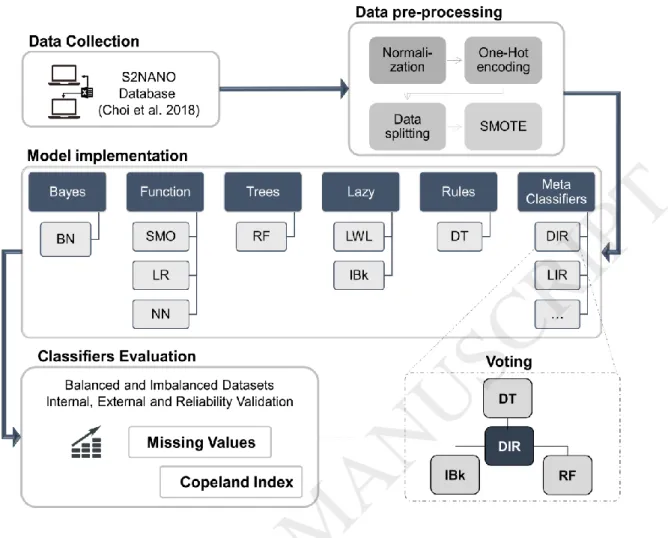
In this study we applied predictive models that estimate NP toxicity based on cell viability following four stages as seen in
Figure 1. These are data collection, data pre-processing, model implementation and model evaluation.
Figure 1. Workflow followed in this study. Datasets are collected from the S2NANO database and processed for ML (normalization, one-hot encoding, data spltting and data synthesis- SMOTE). The training portion of the data is fed to eight base classifiers. Triads of the base classifiers are combined through Voting and the best combinations are used as ensemble classifers. All base and ensemble classifiers are evaluated using internal and external validation and a reliability dataset. In addition, datasets with artificially generated missing values are used to demonstrate the classifiers robustness. Finally, a Copeland Index is used to rank the classifiers. [1.5 column fitting image;]
2.1 Data collection
The two datasets used in this study, originally found in the S2NANO database
(www.s2nano.org), are collected from Choi, Ha [1]. They consist of seven oxide NPs with
physicochemical properties, quantum-mechanical and toxicological attributes and in vitro experimental data (input parameters) reported. The endpoint used as the output to be predicted is simple cytotoxicity of the NP based on cell viability. Information about the dataset can be found in the original paper (ibid). The main (S2NANO data) dataset comprised 574 rows and 16 columns (15 inputs and 1 output). The second dataset (S2NANO reliability validation data in the original paper), originating from studies unrelated to the main dataset, was used for reliability validation. It comprised 144 rows and the same columns as the main dataset. Data attributes of the main dataset are shown in Table 1.
Inputs Parameters Output
Physicochemical attributes
Quantum-Mechanical attributes
Toxicological attributes Toxicity
Core size (nm) 5.9–369 Formation enthalpy (eV) -17.35– -1.61 Assay method 8 types Cell type (normal/cancer) Cell viability (%) (toxic or nontoxic) Hydrodynamic size (nm) 74–1843
Conduction band energy (eV) -5.17– -1.51 Cell name 14 cells Exposure time (h) 3–72 Surface charge (mV) -47.60–42.8
Valence band energy (eV) -11.12 - -6.51
Cell species 3 species
Dose (mg/mL) 0–1440 Specific surface area
(m2/g) 7.0–576.23
Electronegativity (eV) 5.67–6.19
Cell origin 8 types
Table 1. Attributes of the main dataset (S2NANO data) retrieved from Choi, Ha [1] used in the model implementation.
2.2 Data pre-processing
Each input was normalized according to Choi, Ha [1] using z-score, min-max or log10
transformation based on input skewness. Core size, hydrodynamic size, specific surface area, conduction band energy, exposure time and dose were normalized with log10. Surface charge
and formation enthalpy were standardized via z-score. Valence band energy and
electronegativity, were normalized by a min-max method. We used the same normalizations as Choi, Ha [1] in order to be able to compare the classifiers performances generated in this study with the aforementioned. One-Hot encoding was performed for the classifiers which operate only with numeric attributes such as liner regressions. One-Hot encoding is a
technique that converts all nominal attributes into numerical dummy variables (binary) [43]. The value 0 or 1 was used to indicate the absence or presence of the originally nominal attributes. The S2NANO dataset was randomly split into a training (60%) and a validation set (40%) for the classification training and evaluation. The S2NANO training dataset had a class imbalance problem, as it is dominated by experiments of nontoxic class [44]. We balanced the dataset by adjusting the relative frequency of toxic/non-toxic instances by resampling the training dataset applying the Synthetic Minority Oversampling Technique (SMOTE), a supervised instance algorithm that oversamples the minority instances using k-nearest-neighbor (kNN) [45]. The training dataset comprised of 343 rows (Imbalanced Dataset, ID) and reached 575 rows (Balanced Dataset, BD) after applying SMOTE. Later operating SMOTE the training dataset had equally toxic and non-toxic instances. Validation and
reliability datasets comprised of 235 and 144 rows, respectively and SMOTE was not applied to those, since the imbalanced issue is addressed in the training dataset. Learning from data sets that contain few instances of the minority class produces biased classifiers with high predictive accuracy over the majority class, but poorer predictive accuracy over the minority class [46].
2.3 Model implementation
The Weka platform (Waikato Environment for Knowledge Analysis, version 3.8.2) was used for implementing the base and ensemble classifiers [47, 48]. The BD and ID training datasets
were used for implementing the classifiers. Both training datasets were evaluated in order to compare the classifiers in this study with Choi, Ha [1]. Table 2 summarizes the classifiers of this study.
Category Abbreviation Classifier briefly description
Rules DT
Class for building and using a simple Decision Table majority classifier
Bayes BN
Bayes Networks are a type of probabilistic graphical model that uses Bayesian inference for probability computations.
Trees RF
Class for constructing a Forest of Random trees. A tree that considers k-randomly chosen attributes at each node. An ensemble learning method for classification.
Lazy
1. IBk
K-nearest-neighbour Instance-Based learner using Euclidean distance metric.
2. LWL General algorithm for Locally Weighted Learning
Functions
1. NN
Multilayer Perceptron - Neural Network trained with backpropagation
2. SMO
Sequential Minimal Optimization for training a support vector classifier
3. LR Standard Linear Regression for prediction
Table 2. Summary of base and ensemble classifiers used in WEKA.
The eight base classifiers were selected to represent different categories of supervised classifiers such as rules, trees, lazy, functions and bayes. The Vote ensemble method combines the results of base classifiers to provide an optimized prediction.
Rules as a classifier category comprises algorithms that break down the dataset according to rules. Decision table (DT) classifiers hold all links of input data and their outcomes and in case of unknown inputs they use majority value for estimating the outcome, or, as in our application, a nearest neighbour algorithm [49, 50].
Bayes classifiers are probabilistic classifiers [51]. A Bayesian Network (BN) is a directed acyclic graph model that represents variables as nodes and their connections as arcs. Each arc signifies a conditional dependence of the end node to a parent node [52]. The network as a whole represents the joint probability distribution of included variables and use Bayes’ Rule to update conditional probabilities given evidence.
Tree classifiers divide the input value space to a number of paths and sub-paths leading to the class outcomes. Decision trees are constructed using a greedy algorithm that selects the best split point at each step in the tree building process. A decision tree is an efficient
approach used in classification and regression [18]. Random Forest (RF) is a type of ensemble ML algorithm called Bootstrap Aggregation or bagging. An ensemble classifier combines the predictions from several classifiers to increase predictability [53]. Bagging, Boosting and Voting are popular methods for producing ensembles. Bagging produces replicate trainings sets by randomly sampling with replacement from the training instances and combines
classifications of randomly generated training sets to form a final prediction [54, 55]. RF is an improvement upon bagged decision trees that disrupts the greedy splitting algorithm during tree creation so that split points can only be selected from a random subset of the input
attributes [56, 57]. This simple change can decrease the similarity between the bagged trees and in turn the resulting predictions. The final class outcome is then estimated by majority voting of the random trees outcomes [58].
Lazy classifiers are instance-based, they store the data and use them only when needed for the classification. The basic idea behind Locally Weighted Learning (LWL) is that instead of building a global model for the whole function space, for each point of interest a local model is created based on neighbouring data of the query point [59, 60]. For this purpose, each data point becomes a weighting factor which expresses the influence of the data point for the prediction. Instance Based kNN (IBk) is a k nearest neighbour classifier that uses
Euclidean distance and a number of neighbours set by the user.
Algorithms that fall into the functions category include classifiers that can be written as mathematical equations in a reasonably natural way [61]. A NN is a network of
interconnected nodes that propagate the information from the input to the output nodes through the trainable weights of the interconnections and the non-linear function of the nodes [62]. The NN contains one hidden layer and the output layer has one neuron corresponding to toxicity class.
Linear regression (LR) is a simple linear model that minimises the error of a linear formula comprised by adjustable weights for each attribute multiplied by the attribute value [63]. The basic regression method is incapable of discovering nonlinear relationships. Support vector machines (SVM) apply kernel algorithms to transform data to an easier separable form. In our case, the kernel is Sequential Minimal Optimization (SMO) that construct polynomials multiplying attributes and applying adjustable weights to the products. It is a non-linear advancement of linear regression as it actually applies linear regression to a new space of attributes constructed by trying combinations of attribute products [64, 65]. It
uses numeric attributes and can achieve a high degree of accuracy using complex polynomials, thus prone to overfitting.
2.3.1 Voting
Ensemble algorithms iterate and build combinations of base classifiers to improve learning capability [66, 67]. Voting, an ensemble algorithm, provides a simple method for combining base classifiers. The default scheme is to average their probability estimates but in our case the majority voting [68] was used to estimate one value among the outputs of the base
classifiers since it was also used for choosing the classifiers for each ensemble (Table 4). Voting is a commonly used ensemble method for optimizing classification prediction by combining results from individual base classifiers [32, 69-71]
To select which classifiers to use in Voting, we combined all possible sets of three base classifiers1. For each instance and triad, a new predicted value for the toxicity class was calculated based on majority (two out of three) of the predicted values of the three classifiers [73, 74]. The sum of correctly predicted instances for each triad was used to rank the triads and indicate the most complimentary combinations of classifiers. Triads were used to avoid voting risk of ties and to simplify the procedure with respect to processing times and
complexity [32, 75].
2.4 Model Evaluation
Internal validation was performed using 10-fold cross-validation for BD and ID training sets. In 10-fold cross-validation the data is divided randomly into 10 equal sized parts. One part is
1The number of k-combinations of n-elements is computed by the binomial coefficient (n¦k) =n!/k!(n-k)!. For 8 classifiers in triads the number
of possible combinations is (8¦3)=8!/3!(8-3)!=56. 72. Kreher, L., D., and D. Stinston, R.,, Combinatorial algorithms : generation, enumeration, and search, ed. C. Press. 1999, London: CRC Press.
withheld and the algorithm is trained on the remaining nine-tenths; then the error rate is calculated on the holdout set. Finally, the 10 error estimates are averaged to yield an overall estimate. This process aims to reduce randomness of the results and conduct a robust evaluation. The validation data set (40% of S2NANO data) was used for external validation [4]. The reliability dataset was used to test how the models built on data of different origin perform in new situations, predicting the classification of instances from different studies. To evaluate the model predictivity, several performance metrics were considered in addition to correctly classified instances [32]. Those metrics, as seen in Table 3, included the percentage of correct classification for positive rates - toxic (sensitivity, SENS) and non-toxic (specificity, SPEC) and the overall percentage of correct classifications for toxic and non-toxic (balanced accuracy, ACC). F1-score (F1) and Discriminative Power (DP) were also calculated [76, 77].
Balanced Accuracy (ACC) Sensitivity (SENS) Specificity (SPEC) 𝟎. 𝟓 ∗ (𝑻𝑷+𝑭𝑵𝑻𝑷 +𝑭𝑷+𝑻𝑵𝑻𝑵 ) ∗ 𝟏𝟎𝟎% 𝑇𝑃+𝐹𝑁𝑇𝑃 ∗ 100% 𝑇𝑁+𝐹𝑃𝑇𝑁 ∗ 100%
F1 score (F1) Discriminant Power (DP)
𝟐 ∗ 𝑺𝒆𝒏𝒔𝒊𝒕𝒊𝒗𝒊𝒕𝒚 ∗ 𝑷𝒓𝒆𝒄𝒊𝒔𝒊𝒐𝒏𝟏 𝑺𝒆𝒏𝒔𝒊𝒕𝒊𝒗𝒊𝒕𝒚 + 𝑷𝒓𝒆𝒄𝒊𝒔𝒊𝒐𝒏 1𝑷𝒓𝒆𝒄𝒊𝒔𝒊𝒐𝒏 = 𝑻𝑷/(𝑻𝑷 + 𝑭𝑷) √3 𝜋 (𝑙𝑜𝑔 𝑠𝑒𝑛𝑠𝑖𝑡𝑖𝑣𝑖𝑡𝑦 (1−𝑠𝑒𝑛𝑠𝑖𝑡𝑖𝑣𝑖𝑡𝑦)+ 𝑙𝑜𝑔 𝑠𝑝𝑒𝑐𝑖𝑓𝑖𝑐𝑖𝑡𝑦 (1−𝑠𝑝𝑒𝑐𝑖𝑓𝑖𝑐𝑖𝑡𝑦)) Table 3. Definition of classification metrics. TP are the true positive, FN the false negative, TN, the true negative and FP the false positive instances.
In our study, ACC was used to be consistent with Choi et al. [1]. ACC is synonymous with a confusion matrix that shows the number of instances classified correctly as well as
details of misclassifications, or complemented with SENS and SPEC [31]. F-1 score is the weighted average of precision and SENS. Therefore, this score takes both false positives and false negatives into account [78]. Discriminant Power (DP) is a measure that summarizes SENS and SPEC to assess how well a classifier distinguishes between positive and negative cases. The classifier is considered poor for DP <1, limited for 1<DP < 2, fair for 2<DP <3 and good in other cases according to [79].
2.4.1 Missing Values
One of the biggest challenges in predicting NPs toxicity is lack of proper and sufficient information. The lack of standard protocols for NP in vitro toxicity studies [80, 81] results in heterogeneity of data in the literature and, consequently missing values in compiled datasets. Choi, Ha [1] provided a complete dataset having filled the gaps of physicochemical and quantum data in their original source by elaborately combining manufacturer data, theoretical values, and literature data [16]. In order to investigate the robustness of the models when values are missing, we generated versions of the dataset removing values artificially [82, 83]. Three additional training datasets were created from the S2NANO data training set removing values randomly. Probabilities of missing values (0.3, 0.5 and 0.7) were used to define
whether a particular value in an instance was removed e.g., a probability of 0.3 means 30% of the dataset values was replaced with missing data.
2.4.2 Copeland Index
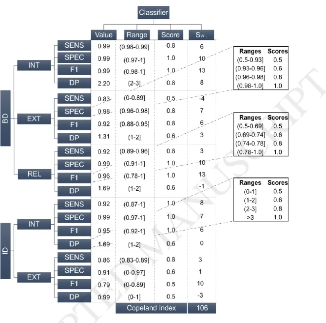
Copeland’s method or Copeland’s pairwise aggregation method ranks candidates which are ordered by the number of pairwise victories (true predictions of toxicity), minus the number of pairwise defeats (false predictions of toxicity) [84-86]. Each classifier was ranked
according to its performance on different datasets (BD, ID), validation processes such as internal (INT), external (EXT) and realibility (REL) and performance metrics such as
sensitivity (SENS), specificity (SPEC), F1-score (F1) and Discriminant Power (DP) (see Figure 2).
The performance value from each metric individually, except DP, were discretized into bins of equally frequenced values. DP bin-ranges were defined according to their evaluation meaning as explained in 2.4 . Bins were used to filter out small differences that the Copeland Index would enhance. Each bin got a score in the same range (0.5 to 1 being an appropriate scale) so that different metrics can be compared and aggregated. This score was used to calculate the win-loss scores of the classifier for each case (e.g. BD-INT-SENS). The win-loss score, SW-L, is the count of wins minus the count of losses when comparing the classifier with the other classifiers. Copeland Index is the sum of win-loss scores for all datasets and validations for one classifier [87-89]. In total, 20 values of SW-L (five validation processess for two different datasets) were added per classifier to provide the Copeland Index (Figure 2). Reliability validation was performed only with BD in order to compare the classifiers with Choi, Ha [1].
Figure 2. Copeland Index compilation. Examples of ranges and range scoring of specficity, F1-score and DP. The ranges were defined by discretizing equally the results from the classifiers in four sections. DP ranges are based on Sokolova, Japkowicz [79] and are the same across different datasets and validation processes.[single column fitting image;]
3 Results 3.1 Voting
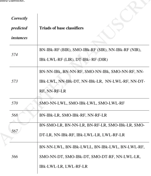
Table 4 presents the ranking of the base classifier triads according to the number of correctly predicted instances. Five triads get a perfect score (574/574), all combining IBk and RF with a third classifier.
Correctly predicted instances
Triads of base classifiers
574
BN-IBk-RF (BIR), SMO-IBk-RF (SIR), NN-IBk-RF (NIR), IBk-LWL-RF (LIR), DT-IBk- RF (DIR)
573
BN-IBk, BN-RF, SMO-IBk, SMO-RF, NN-IBk-LWL, NN-IBk-DT, NN-IBk-LR, NN-LWL-RF, NN-DT-RF, NN-RF-LR
570 SMO-NN-LWL, SMO-IBk-LWL, SMO-LWL-RF 568 BN-IBk-LR, SMO-IBk-RF, NN-RF-LR
567
BN-LR, BN-NN-LR, BN-RF-LR, IBk-LR, SMO-DT-LR, NN-IBk-RF, IBk-LWL-LR, LWL-RF-LR
566
BN-NN-LWL, BN-IBk-LWLL, BN-IBk-LWL, BN-LWL-RF, SMO-NN-DT, SMO-IBk-DT, SMO-DT-RF, NN-LWL-LR, IBk-LWL-LR, LWL-RF-LR
Table 4 Ranking of base classifier triads according to correctly predicted instances for training datasets. An instance is considered correctly predicted by a triad when it is correctly predicted by at least two of its members. The total number of instances in dataset is 574..
3.2 Classifier Evaluation
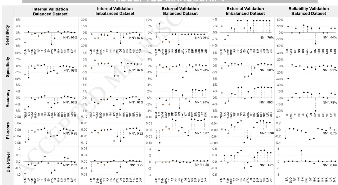
The classification performance of the models is presented in Figure 3. It shows the results of the eight base models, including the models (*) from Choi, Ha [1], and of the five perfect scoring triads of the voting (BIR, SIR, NIR, LIR, DIR) across all datasets and classification metrics.
Figure 3. Base models and Voting triads relative performances for different dataset and metrics. Axis x (y=0) in each graph represents a Neural Network, NN*, the best performing model in Choi, Ha [1]. The lollipops represent the differences between the classifiers and the NN*. The absolute performance of NN* is given for each case. Performance of models with * (orange dots) are based on model results as reported in Choi, Ha [1]. [2-column fitting image;]
Internal Balanced Dataset
LWL and Generalized Linear Model (GLM*) have the lowest SENS comparing to NN* (≈ -7%) and DT has -3% SENS. All other base and ensemble classifiers have similar SENS performance with NN*(±1%). LR, BN, DT and lazy classifiers have lower SPEC differing to NN* from -13% to -5% and lower ACC ranging from -6% to -3%. DIR enesmble classifier has -2% SPEC difference. On the other hand, NN has 2% higher SENS compared to NN*. All other base and ensemble classifiers have almost same SPEC and ACC performance (±1%). LR has lower F1 than the other classifiers (-0.06). NN has the highest DP improvement (+0.39) in contrast with LWL (-0.85). Summing up, LR, DT, BN and lazy classifiers do not perform as well for almost all metrics. All ensemble classifiers have similar performance to the best base classifiers, NN and RF (See Figure 3 first column).
Internal Imbalanced Dataset
BN, DT, RF, IBk and function classifiers have lower SENS comparing to NN*. DT reached the lowest score (24%) and the rest circa 8%. NN and LWL have ≈ +3% SENS. DIR has -4% SENS while all the other ensembles have ≈ +1% SENS except BIR (-2%). BN and lazy classifiers have lower SPEC (≈ -4%). All other base and ensemble classifiers have ≈ +1% SPEC performance with LR reaching +3%. BN and DT have the lowest ACC and F1. LR and IBk have -6% ID ACC. NN classifier has +2% ACC. The rest of base classifiers and DIR have -2% ACC. The ensemble classifiers have good ACC performance (±1%) and higher F1 score. LR and ensemble classifiers (except DIR) have higher DP. Summing up, all base classifiers, except NN and LWL, have lower SENS. BN and lazy classifiers have also lower SPEC and ACC. Ensemble classifiers, DIR excluded, have +1% higher performance (see Figure 3 second column).
External Balanced Dataset
BN and SMO have lower SENS, -9% and -5% respectively, with LR reaching the highest, +7%. All other base and ensemble classifiers have almost same SENS performance (±1%). LR have lower SPEC than NN*. BN has the lowest ACC (-3%). RF, NN and all the ensemble classifiers reach +5% higher SPEC, +2% higher ACC, higher F1 (≈ + 0.08) and DP scores (≈ + 0.38). LR has the lowest F1 score (-0.1) and the highest DP (>3). Summing up, NN and RF and ensemble classifiers have the best performance. BN has the lowest performance (see Figure 3 third column).
External Imbalanced Dataset
All classifiers outperformed NN* SENS except LR (-7%). The highest score is reached by LWL, IBk, RF, NN and ensemble classifiers (+13%). DT, BN and LWL have lower SPEC than NN* (≈ -5%). In contrast, all other base and ensemble classifiers have almost the same SPEC performance (±1%). LR is the only classifier having lower ACC (-3%). RF, NN and ensemble classifiers have +7% higher ACC with SIR and NIR reaching the highest. NN, SIR and NIR have the highest F1 score (+0.06) and DP (+0.45). BN and DT have the lowest (-0.08 and -0.24 for F1 and DP respectively). Summing up, LR has the lowest performane. DT, BN and LWL have lower SPEC. The ensemble classifiers reach the highest SENS and SPEC while SIR and NIR reach the highest ACC (see Figure 3 fourth column).
Reliabillity Dataset
BN reaches the highest SENS (+36%) and IBk the lowest (-50%). LR and LWL have +29% difference while RF, DT, BIR, LIR and SIR reach +22% from NN* (64%). LR scores the lowest (-38%) and SMO the highest (+4%) SPEC. All classifiers have lower SPEC than NN*. BN and LWL classifiers have the highest ACC (+13%) while IBk reaches the lowest (-30%). LIR has among the highest ACC (+11%), F1 (+0.06) and DP (+0.33). DT has the lowest F1
score (-0.3) and IBk the lowest DP (-0.75). Summing up, BN has the highest SENS (36%) and IBk the lowest (-50%). SIR and SMO have the highest SPEC. BN, LWL and LIR have the highest ACC (see Figure 3 last column).
3.3 Missing Values
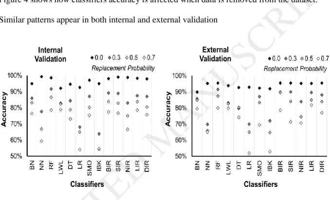
Figure 4 shows how classifiers accuracy is affected when data is removed from the dataset. Similar patterns appear in both internal and external validation
Figure 4. Robustness of classifiers in case of missing data. Internal (left) and external (right) balanced accuracy for datasets with different replacement probabilities of missing
values.Vertically packed dots show that the model maintains accuracy in scarce datasets. [single- column fitting image].
RF model has the best internal ACC performance from all models reaching 92% with 0.3 missing values dataset and 88% with the 0.5 dataset. BN, LWL and RF have the least span among the base classifiers showing they are the least affected models. In general, ensemble classifiers perform better with NIR being the least robust. SIR performs equally with DIR at
all points of probabilities. At probability of 0.5 missing values, BN starts perform better that the ensemble classifiers. NN starts with high ACC, but it is quite sensitive to missing data compared to all other models. RF, LWL and BN are able to handle missing values datasets, even at 0.7. LIR outperforms the other models at 0.7 reaching 82% ACC at external validation and equal performance with RF and LWL at internal validation (79%). RF has the most robust performance reaching 92% ACC when 30% of dataset values are removed and maintaining 88% accuracy with a 0.5 dataset.
3.4 Copeland Index
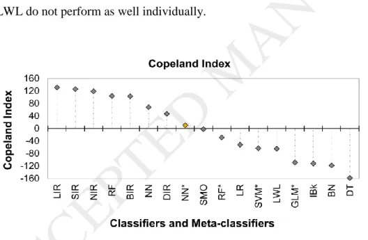
The best classifier based on the Copeland Index integrating all metrics and datasets is the ensemble classifier LIR (LWL-IBk-RF) (Figure 5). RF is the best base classifier but IBk and LWL do not perform as well individually.
Figure 5. Scoring of base and ensemble classifiers across the four basic criteria: metric scoring, performance metric, validation and dataset. Classifiers are orderded from highest ranking (left) to lower (right). NN* the best classifier from Choi, Ha [1] is shown with orange dot [single- column fitting image].
RF and NN have the highest performances among the base classifiers and perform better still when combined (NIR). SIR is the second best ensemble classifier. SMO has an
average performance scoring same number of wins and losses but combined with IBk and RF the performance is significantly enhanced. Combining RF with the BN or DT, in BIR and DIR respectively worsens the performance of RF.
4 Discussion
In this study we demonstrate a methodology to select the best combinations of base classifiers for ensemble classifier using voting. Base classifiers are combined in triads and ranked according to their best accuracies calculated by majority voting. The best combinations of classifiers are used to implement voting ensemble classifiers. In this study we used a voting method of correctly predicted values for combining classifiers in triad ensembles. Using also triads, Tamvakis et al (2018) propose a general dissimilarity index. The complexity of
combinations with more than three classifiers is not applied in this study and is likely to prove unwieldy.
Regarding base classifiers, RF and NN showed the best performance in contrast to LWL and IBk which showed the lowest performance. Linear regression classifiers (LR, GLM*) performance is poor for most metrics and the Copeland Index. Simple linearity cannot predict toxicity when independent variables vary. Support vector machines capture these variations much better, applying linear regression after combining attributes to form a more separable dataset.
Trees (RF, RF*) and NN are the best base classifiers; RF has a better performance than NN in some cases, such as in EXT ID validation or REL. RF decreases the variance through bootstrap aggregation (ensemble-algorithm that improves accuracy, bagging) resulting in good prediction capabilities and ranking RF as the best base classifier.
The IBk classifier performs moderately. Its kNN algorithm however, using weighted distance, is capable of correctly predicting instances that other classifiers may not predict. Supplementing each other, IBk and RF are always the two best base classifiers in all best triad combinations. RF is already a strong bagging classifier able to predict the majority of
instances. Combinations of a base classifiers with RF and IBk, predict specific instances that are unpredicted by the best base classifiers. In our case, LIR, that is, majority voting among a bagging classifier, RF, and two lazy classifiers, IBk and LWL, gives the best results, as reflected also in the Copeland Index. These results point towards combining more robust with simpler classifiers and using bagging (RF and Voting) [90].
The RF and NN classifiers applied in this study perform better than RF* and NN* from Choi, Ha [1]. This may be attributed to the 60-40 split of the original dataset for training and validation and mostly to the classifier parameters set-up. Choi, Ha [1] do not provide details on the classifier parameters therefore an accurate reproduction using their classifiers is not possible. For instance, the number of hidden layers in NN and tree depth in RF used in this study may vary.
Bayes Network has excellent results in the reliability validation but moderate in the external validation. The dataset used in this study is designed for a QSAR application, using numerical attributes. Bayes Networks operate on nominal attributes; in this study, we discretize the numeric attributes into nominal ranges. Discretization was performed on the final training dataset so attribute values in the reliability or validation data may correctly be predicted according to the training ranges. In the ensemble (BIR) classifier, BN improves all its metrics and ranks third in the Copeland Index.
The best triad (LIR) shows a high performance across most datasets, particularly the overall performance for reliability dataset. Other triads, that included the best base classifiers,
did not performed well with the reliability dataset. For the three datasets, the best triad shows an improvement in classification performance in all cases, especially in external validation. The goal of this study is to test classifiers on reaching an overall good performance referring to all datasets and metrics combined, avoiding overfitting and underfitting. In this respect, ensemble methods produce the best results compared to base classifiers. Classifier
performance differs by class balance (BD, ID), validation process (internal, external, reliability) and the performance metric considered (e.g. sensitivity, precision). We integrate all cases in a Copeland Index to compare classifiers in a singular ranking.
The Copeland Index clearly reveals ensemble classifiers have higher scores than base classifiers, confirming the results in Figure 3, voting’s potential to increase the predictive ability. The best classifier in this ranking (LIR) did not contain the two best base classifiers combined (e.g. NIR).
Model performances corresponding to datasets with missing values are not included in the Copeland Index. The generation of missing values is random and does not account for joint probabilities of missing data (e.g. all quantum-mechanical values missing as not measured in an experiment) due to the experimental design. Missing values in toxicological datasets is a common issue that modellers have to deal with. We tested the model
performance with different replacement probabilities of missing values. BN, LWL, RF and SMO base classifiers can perform well maintaining their accuracy levels to those using the dataset with no missing values. As expected, Bayes networks and the Naïve Bayes classifiers in LWL handle missing values well [91]. RF through randomising and bagging and SMO through combining attributes, manage to rebuild the toxicological outcome through attribute interrelations. BIR, SIR, LIR and DIR also demonstrate robustness despite missing values. NN, although accurate in whole dataset predictions, show poor performance when values are
missing. IBk and LR have also very poor performances. LIR has a very robust behaviour competing with RF. Similar conclusions can be drawn for the external validation, with SIR having the best accuracy, preforming better than RF. Values were randomly removed in this study while in real-world datasets missing values correspond to omissions or limitations in the experimental protocols and designs. The robustness of the model performance on missing data should be tested in real datasets where no information for systematically missing for specific attributes instead of randomly distributed values in the dataset.
In most existing databases several issues such as, data curation (quality and
completeness), common ontology, format of datasets, missing values (grouping approaches) etc., are not handled. Basei, Hristozov [92] provides an overview on databases, highlighting the importance of data curation showing that more efforts are needed to develop reliable datasets. In this scope, an integrated science-based framework under the GRACIOUS project (https://www.h2020gracious.eu/) is currently being built. The curation system of GRACIOUS is targeting existing data that will go through quality assessments.
A dataset derived from the S2NANO database was selected for this study. S2NANO integrates data form different sources and handles the aforementioned data quality issues making the dataset fit for testing models. The specific dataset is curated (quality data and completeness are assessed and handled) and has been used before for predicting toxicity using ML models [1]. Results of the latter served as a reference point for testing and demonstrating our methodology.
Using datasets from the GRACIOUS project database when available or testing the methodology on existing high quality datasets of different case studies including multiple toxicological outcomes [10, 17, 93-95], are the next steps to demonstrate the validity and
robustness of our concept. Classifiers used previously on the data can be included in the implementation and participate in the ranking process.
5 Conclusions
In this study, we demonstrated the performance of many classifiers on extracts of a specific toxicological dataset. Ensembles of those classifiers were compiled based on combined performance. Major voting ensemble classifiers were applied in the same dataset and were found to outperform base classifiers. The classifiers were ranked according to a Copeland Index based on all basic criteria of the analysis, such a datasets, validation processes and performance metrics. Bagging, reducing the variance of the classifiers, results to better results in tree classifiers and all ensemble classifiers; the best ensembles included one accurate base classifier with simpler “satellite” classifiers that predict the outlying instances. Classifier comparison on datasets with artificially removed values demonstrated that ensemble
classifiers based on voting algorithm where still able to perform acceptably even when most values in a dataset were missing.
Declaration of interests
The authors declare that they have no known competing financial interests or personal relationships that could have appeared to influence the work reported in this paper.
Acknowledgments
This work was supported by the European Union’s Horizon 2020 research and innovation programme [grant number 720851]. CAP was funded by the Colt Foundation.
REFERENCES
1. Choi, J.-S., et al., Towards a generalized toxicity prediction model for oxide nanomaterials
using integrated data from different sources. Scientific Reports, 2018. 8(1): p. 6110.
2. Khan, I., K. Saeed, and I. Khan, Nanoparticles: Properties, applications and toxicities. Arabian Journal of Chemistry, 2017.
3. Jeevanandam, J., et al., Review on nanoparticles and nanostructured materials: history,
sources, toxicity and regulations. Beilstein journal of nanotechnology, 2018. 9: p. 1050-1074.
4. Raies, A.B. and V.B. Bajic, In silico toxicology: computational methods for the prediction of
chemical toxicity. Wiley Interdisciplinary Reviews. Computational Molecular Science, 2016. 6(2): p.
147-172.
5. Watson, C., et al., High-throughput screening platform for engineered nanoparticle-mediated
genotoxicity using CometChip technology. ACS nano, 2014. 8(3): p. 2118-2133.
6. Damoiseaux, R., et al., No time to lose--high throughput screening to assess nanomaterial
safety. Nanoscale, 2011. 3(4): p. 1345-1360.
7. Sharifi, S., et al., Toxicity of nanomaterials. Chemical Society reviews, 2012. 41(6): p. 2323-2343.
8. Aillon, K.L., et al., Effects of nanomaterial physicochemical properties on in vivo toxicity.
Advanced Drug Delivery Reviews, 2009. 61(6): p. 457-466.
9. Nel, A.E., et al., Understanding biophysicochemical interactions at the nano–bio interface.
Nature Materials, 2009. 8: p. 543.
10. Concu, R., et al., Probing the toxicity of nanoparticles: a unified in silico machine learning
model based on perturbation theory. Nanotoxicology, 2017. 11(7): p. 891-906.
11. Sizochenko, N., et al., How the toxicity of nanomaterials towards different species could be
simultaneously evaluated: a novel multi-nano-read-across approach. Nanoscale, 2018. 10(2): p.
582-591.
12. Furxhi, I., et al., Bayesian Networks application for the prediction of cellular effects from
genome-wide transcriptomics studies of exposure to Nanoparticles. 2019, University of Limerick.
13. Quik, J.T.K., et al., Directions in QPPR development to complement the predictive models used
in risk assessment of nanomaterials. NanoImpact, 2018. 11: p. 58-66.
14. Trinh, T.X., et al., Curation of datasets, assessment of their quality and completeness, and
nanoSAR classification model development for metallic nanoparticles. Environmental Science: Nano,
2018.
15. Karcher, S., et al., Integration among databases and data sets to support productive
nanotechnology: Challenges and recommendations. NanoImpact, 2018. 9: p. 85-101.
16. Ha, M.K., et al., Toxicity Classification of Oxide Nanomaterials: Effects of Data Gap Filling
and PChem Score-based Screening Approaches. Scientific Reports, 2018. 8: p. 3141.
17. Kleandrova, V.V., et al., Computational Tool for Risk Assessment of Nanomaterials: Novel QSTR-Perturbation Model for Simultaneous Prediction of Ecotoxicity and Cytotoxicity of Uncoated
and Coated Nanoparticles under Multiple Experimental Conditions. Environmental Science &
Technology, 2014b. 48(24): p. 14686-14694.
18. Bhavna, S. and S. Sumit, Nanotoxicity prediction using computational modelling - review and
future directions. IOP Conference Series: Materials Science and Engineering, 2018. 348(1): p.
012005.
19. Findlay, M.R., et al., Machine learning provides predictive analysis into silver nanoparticle
protein corona formation from physicochemical properties. Environmental Science: Nano, 2018. 5(1):
p. 64-71.
20. Sheehan, B., et al., Hazard Screening Methods for Nanomaterials: A Comparative Study.
International Journal of Molecular Sciences, 2018. 19(3): p. 649.
21. Schöning, V., S. Krähenbühl, and J. Drewe, The hepatotoxic potential of protein kinase
inhibitors predicted with Random Forest and Artificial Neural Networks. Toxicology Letters, 2018.
299: p. 145-148.
22. Li, Y., et al., Drug interaction study of flavonoids toward CYP3A4 and their quantitative
structure activity relationship (QSAR) analysis for predicting potential effects. Toxicology Letters,
2018. 294: p. 27-36.
23. Pastor, M., et al., Development and validation of computational models for predicting oxidative
stress responses using comprehensive series of drug-like compounds. Toxicology Letters, 2018. 295:
p. S62-S63.
24. Gómez-Tamayo, J.C., et al., Ligand based and structural based modeling for the understanding,
classification and prediction ofmitochondrial toxicity. Toxicology Letters, 2018. 295: p. S96.
25. Low-Kam, C., et al., A Bayesian regression tree approach to identify the effect of nanoparticles’
properties on toxicity profiles. The Annals of Applied Statistics, 2015. 9(1): p. 383-401.
26. Marvin, H.J.P., et al., Application of Bayesian networks for hazard ranking of nanomaterials to
support human health risk assessment. Nanotoxicology, 2017. 11(1): p. 123-133.
27. Murphy, F., et al., A Tractable Method for Measuring Nanomaterial Risk Using Bayesian
Networks. Nanoscale Research Letters, 2016. 11: p. 503.
28. Puzyn, T., et al., Perspectives from the NanoSafety Modelling Cluster on the validation criteria
for (Q)SAR models used in nanotechnology. Food and Chemical Toxicology, 2018. 112: p. 478-494.
29. Burello, E., Review of (Q)SAR models for regulatory assessment of nanomaterials risks.
NanoImpact, 2017. 8: p. 48-58.
30. Ventura, C., D.A.R.S. Latino, and F. Martins, Comparison of Multiple Linear Regressions and
Neural Networks based QSAR models for the design of new antitubercular compounds. European
Journal of Medicinal Chemistry, 2013. 70: p. 831-845.
31. Kovalishyn, V., et al., Modelling the toxicity of a large set of metal and metal oxide
nanoparticles using the OCHEM platform. Food and Chemical Toxicology, 2018. 112: p. 507-517.
32. Tamvakis, A., et al., Optimized Classification Predictions with a New Index Combining
Machine Learning Algorithms. International Journal on Artificial Intelligence Tools, 2018. 27(03): p.
1850012.
33. B., R.A. and B.V. B., In silico toxicology: comprehensive benchmarking of multi-label
classification methods applied to chemical toxicity data. Wiley Interdisciplinary Reviews:
Computational Molecular Science, 2018. 8(3): p. e1352.
34. Ai, H., et al., Predicting Drug-Induced Liver Injury Using Ensemble Learning Methods and
Molecular Fingerprints. Toxicological Sciences, 2018: p. kfy121-kfy121.
35. Jain, S., E. Kotsampasakou, and G.F. Ecker, Comparing the performance of meta-classifiers—a
case study on selected imbalanced data sets relevant for prediction of liver toxicity. Journal of
Computer-Aided Molecular Design, 2018. 32(5): p. 583-590.
36. Cerruela García, G., et al., Molecular activity prediction by means of supervised subspace
projection based ensembles of classifiers. SAR and QSAR in Environmental Research, 2018. 29(3): p.
187-212.
37. Zaslavskiy, M., et al., ToxicBlend: Virtual screening of toxic compound with ensemble
predictors. Toxicology Letters, 2018. 295: p. S98.
38. Kazemi, Y. and S.A. Mirroshandel, A novel method for predicting kidney stone type using
ensemble learning. Artificial Intelligence in Medicine, 2018. 84: p. 117-126.
39. Hooda, N., S. Bawa, and P.S. Rana, B2FSE framework for high dimensional imbalanced data:
A case study for drug toxicity prediction. Neurocomputing, 2018. 276: p. 31-41.
40. Chernova, T., et al., Long-Fiber Carbon Nanotubes Replicate Asbestos-Induced Mesothelioma
with Disruption of the Tumor Suppressor Gene Cdkn2a (Ink4a/Arf). Current Biology, 2017. 27(21): p.
3302-3314.e6.
41. Haase, A., & Klaessig, F.,, EU US Roadmap Nanoinformatics 2030, in EU Nanosafety Cluster. 2018.
42. Papa, E., et al., Investigation of the influence of protein corona composition on gold
nanoparticle bioactivity using machine learning approaches. SAR QSAR Environ Res, 2016. 27(7): p.
521-38.
43. Cassel, M. and F. Lima. Evaluating one-hot encoding finite state machines for SEU reliability
in SRAM-based FPGAs. in 12th IEEE International On-Line Testing Symposium (IOLTS'06). 2006.
44. Wang, S.-H., et al., Classification Methods for Pathological Brain Detection, in Pathological
Brain Detection. 2018, Springer Singapore: Singapore. p. 119-147.
45. Chawla, N.V., et al., SMOTE: Synthetic Minority Oversampling TEchnique. Journal of Artificial Intelligence Research, 2002(16): p. 321-357.
46. Hu, S., et al. MSMOTE: Improving Classification Performance When Training Data is
Imbalanced. in 2009 Second International Workshop on Computer Science and Engineering. 2009.
47. Hall, M., et al., The WEKA data mining software: an update. SIGKDD Explor. Newsl., 2009.
11(1): p. 10-18.
48. El-Melegy, M.T., et al. A comparative study of classification methods for automatic multimodal
brain tumor segmentation. in 2018 International Conference on Innovative Trends in Computer
Engineering (ITCE). 2018.
49. AbouEisha, H., et al., Different Kinds of Decision Trees, in Extensions of Dynamic
Programming for Combinatorial Optimization and Data Mining. 2019, Springer International
Publishing: Cham. p. 35-48.
50. Amandi, A., Ryan J. Urbanowicz, and Will N. Browne: Introduction to learning classifier
systems. Genetic Programming and Evolvable Machines, 2018. 19(4): p. 569-570.
51. Friedman, N., D. Geiger, and M. Goldszmidt, Bayesian Network Classifiers. Mach. Learn., 1997. 29(2-3): p. 131-163.
52. Xu, S., Bayesian Naïve Bayes classifiers to text classification. Journal of Information Science, 2018. 44(1): p. 48-59.
53. Dietterich, T.G., An Experimental Comparison of Three Methods for Constructing Ensembles of
Decision Trees: Bagging, Boosting, and Randomization. Machine Learning, 2000. 40(2): p. 139-157.
54. Zareapoor, M. and P. Shamsolmoali, Application of Credit Card Fraud Detection: Based on
Bagging Ensemble Classifier. Procedia Computer Science, 2015. 48: p. 679-685.
55. Sun, Q. and B. Pfahringer. Bagging Ensemble Selection. 2011. Berlin, Heidelberg: Springer Berlin Heidelberg.
56. Esmaily, H., et al., A Comparison between Decision Tree and Random Forest in Determining
the Risk Factors Associated with Type 2 Diabetes. 2018. Vol. 18. 2018.
57. Hengl, T., et al., Random forest as a generic framework for predictive modeling of spatial and spatio-temporal variables. PeerJ, 2018. 6: p. e5518.
58. Breiman, L., Random Forests. Machine Learning, 2001. 45(1): p. 5-32.
59. Englert, P., Locally Weighted Learning. Seminar Class on Autonomous Systems, 2012. 60. Kaur, P. and P. Rani, Investigation of Lazy Classification in Data Mining using WEKA tool.
International Journal of Scientific Research in Computer Science, Engineering and Information Technology, 2018. 3(3).
61. Witten, I.H., et al., Data Mining, Fourth Edition: Practical Machine Learning Tools and
Techniques. 2016: Morgan Kaufmann Publishers Inc. 654.
62. Zhang, Z., Artificial Neural Network, in Multivariate Time Series Analysis in Climate and
Environmental Research. 2018, Springer International Publishing: Cham. p. 1-35.
63. Cattaneo, M.D., M. Jansson, and W.K. Newey, Inference in Linear Regression Models with
Many Covariates and Heteroscedasticity. Journal of the American Statistical Association, 2017: p.
1-12.
64. Sørensen, L. and M. Nielsen, Ensemble support vector machine classification of dementia using
structural MRI and mini-mental state examination. Journal of Neuroscience Methods, 2018. 302: p.
66-74.
65. Gao, X., L. Fan, and H. Xu, Multiple rank multi-linear kernel support vector machine for matrix
data classification. International Journal of Machine Learning and Cybernetics, 2018. 9(2): p.
251-261.
66. Ali, R., et al., A Case-Based Meta-Learning and Reasoning Framework for Classifiers
Selection, in Proceedings of the 12th International Conference on Ubiquitous Information
Management and Communication. 2018, ACM: Langkawi, Malaysia. p. 1-6.
67. Nakano, F.k., et al. Stacking Methods for Hierarchical Classification. in 2017 16th IEEE
International Conference on Machine Learning and Applications (ICMLA). 2017.
68. Lam, L. and S.Y. Suen, Application of majority voting to pattern recognition: an analysis of its
behavior and performance. IEEE Transactions on Systems, Man, and Cybernetics - Part A: Systems
and Humans, 1997. 27(5): p. 553-568.
69. Zhang, L., et al., CarcinoPred-EL: Novel models for predicting the carcinogenicity of chemicals
using molecular fingerprints and ensemble learning methods. Scientific Reports, 2017. 7(1): p. 2118.
70. Raies, A.B. and V.B. Bajic, In silico toxicology: comprehensive benchmarking of multi-label
classification methods applied to chemical toxicity data. Wiley Interdisciplinary Reviews:
Computational Molecular Science, 2017. 8(3): p. e1352.
71. Mikolajczyk, A., et al., Zeta Potential for Metal Oxide Nanoparticles: A Predictive Model
Developed by a Nano-Quantitative Structure–Property Relationship Approach. Chemistry of
Materials, 2015. 27(7): p. 2400-2407.
72. Kreher, L., D., and D. Stinston, R.,, Combinatorial algorithms : generation, enumeration, and
search, ed. C. Press. 1999, London: CRC Press.
73. Rokach, L., Ensemble-based classifiers. Artificial Intelligence Review, 2010. 33(1): p. 1-39. 74. Afolabi, L.T., et al., Ensemble learning method for the prediction of new bioactive molecules.
PLOS ONE, 2018. 13(1): p. e0189538.
75. Banfield, R.E., et al., Ensemble diversity measures and their application to thinning.
Information Fusion, 2005. 6(1): p. 49-62.
76. Li, Y., et al., 4D-Fingerprint Categorical QSAR Models for Skin Sensitization Based on
Classification Local Lymph Node Assay Measures. Chemical research in toxicology, 2007. 20(1): p.
114-128.
77. Contrera, J.F., et al., Comparison of MC4PC and MDL-QSAR rodent carcinogenicity
predictions and the enhancement of predictive performance by combining QSAR models. Regulatory
Toxicology and Pharmacology, 2007. 49(3): p. 172-182.
78. Reilly, M.A.O., et al. The influence of feature selection methods on exercise classification with
inertial measurement units. in 2017 IEEE 14th International Conference on Wearable and
Implantable Body Sensor Networks (BSN). 2017.
79. Sokolova, M., N. Japkowicz, and S. Szpakowicz. Beyond Accuracy, F-Score and ROC: A
Family of Discriminant Measures for Performance Evaluation. 2006. Berlin, Heidelberg: Springer
Berlin Heidelberg.
80. Drasler, B., et al., In vitro approaches to assess the hazard of nanomaterials. NanoImpact, 2017. 8: p. 99-116.
81. Warheit, D.B., Hazard and risk assessment strategies for nanoparticle exposures: how far have
we come in the past 10 years? F1000Research, 2018. 7: p. 376.
82. Farhangfar, A., L. Kurgan, and J. Dy, Impact of imputation of missing values on classification
error for discrete data. Pattern Recognition, 2008. 41(12): p. 3692-3705.
83. Witten, I.H., et al., Weka: Practical machine learning tools and techniques with Java
implementations, in Computer Science Working Papers. 1999.
84. Sculley, D., Rank Aggregation for Similar Items, in Proceedings of the 2007 SIAM International
Conference on Data Mining. 2006. p. 587-592.
85. Cook, W.D., Distance-based and ad hoc consensus models in ordinal preference ranking.
European Journal of Operational Research, 2006. 172(2): p. 369-385.
86. Al-Sharrah, G., Ranking Using the Copeland Score: A Comparison with the Hasse Diagram.
Journal of Chemical Information and Modeling, 2010. 50(5): p. 785-791.
87. Koch, S. and J. Mitlöhner, Software project effort estimation with voting rules. Decision Support Systems, 2009. 46(4): p. 895-901.
88. Ragothaman, S., B. Naik, and K. Ramakrishnan, Predicting Corporate Acquisitions: An
Application of Uncertain Reasoning Using Rule Induction. Information Systems Frontiers, 2003. 5(4):
p. 401-412.
89. Xia, L., Generalized scoring rules: a framework that reconciles Borda and Condorcet.
SIGecom Exch., 2013. 12(1): p. 42-48.
90. Galar, M., et al., A Review on Ensembles for the Class Imbalance Problem: Bagging-,
Boosting-, and Hybrid-Based Approaches. IEEE Transactions on Systems, Man, and Cybernetics, Part C
(Applications and Reviews), 2012. 42(4): p. 463-484.
91. Friedman, N., Learning Belief Networks in the Presence of Missing Values and Hidden
Variables, in Proceedings of the Fourteenth International Conference on Machine Learning. 1997,
Morgan Kaufmann Publishers Inc. p. 125-133.
92. Basei, G., et al., Making use of available and emerging data to predict the hazards of
engineered nanomaterials by means of in silico tools: A critical review. NanoImpact, 2019. 13: p.
76-99.
93. Kleandrova, V.V., et al., Computational ecotoxicology: Simultaneous prediction of ecotoxic
effects of nanoparticles under different experimental conditions. Environment International, 2014. 73:
p. 288-294.
94. Furxhi, I., et al., Application of Bayesian Networks in Determining Nanoparticle Induced
Cellular Outcomes Using Transcriptomics. 2019: Manuscript accepted in Nanotoxicology Journal.
95. Basant, N. and S. Gupta, Multi-target QSTR modeling for simultaneous prediction of multiple
toxicity endpoints of nano-metal oxides. Nanotoxicology, 2017. 11(3): p. 339-350.
6 Data references
Datasets: Jang-Sik Choi, My Kieu Ha, Tung Xuan Trinh, Tae Hyun Yoon & Hyung-Gi Byun, S2NANO data and S2NANO reliability validation data, Nature Scientific Reports, 2018.
![Table 1. Attributes of the main dataset (S2NANO data) retrieved from Choi, Ha [1] used in the model implementation](https://thumb-us.123doks.com/thumbv2/123dok_us/9741265.2465280/11.892.97.797.420.896/table-attributes-dataset-nano-retrieved-choi-model-implementation.webp)