must be obtained for all other uses, in any current or future media, including reprinting/republishing this material for advertising or promotional purposes, creating new collective works, for resale or redistribution to servers or lists, or reuse of any copyrighted component of this work in other works.”
CogBoost: Boosting for Fast Cost-sensitive
Graph Classification
Shirui Pan, Jia Wu, and Xingquan Zhu,
Senior Member, IEEE
Abstract—Graph classification has drawn great interests in recent years due to the increasing number of applications involving objects with complex structural relationships. To date, all existing graph classification algorithms assume, explicitly or implicitly, that misclassifying instances in different classes incurs an equal amount of cost/risk, which is often not the case in real-life applications (where misclassifying a certain class of samples, such as diseased patients, is subject to more expensive costs than others). Although cost-sensitive learning has been extensively studied, all methods are based on data with instance-feature representation. Graphs, however, do not have features available for learning and the possible feature space of graph data are likely infinite and needs to be carefully explored in order to favor classes with a higher cost. Furthermore, current graph classification models are designed for small graph datasets and can hardly scale to the increase of the training set size. In this paper, we propose, CogBoost, a fast cost-sensitive graph classification algorithm, where the goal is to minimize the misclassification costs (instead of the errors) and to achieve fast learning speed for large scale graph datasets. To minimize the misclassification costs, CogBoost iteratively selects the most discriminative subgraph by considering costs of different classes, and then solves a linear programming problem in each iteration by using Bayes decision rule based optimal loss function. In addition, a cutting plane algorithm is derived to speed up the solving of linear programs for fast learning on large graph datasets. Experiments and comparisons on real-world large graph datasets demonstrate the effectiveness and the efficiency of our algorithm.
Index Terms—Graph classification, Cost-sensitive learning, Subgraphs, Boosting, Cutting plane algorithm, Large scale graphs
F
1
I
NTRODUCTIOND
UE to the rapid advancement in the data collection technology, recent years have witnessed an increasing number of applications with complex structural relation-ships inside the data, e.g., chemical compounds [1], so-cial networks [2], and scientific publications [3]. Different from traditional data which are represented in deterministic feature space by using an instance-feature representation, structural data are not represented by using attribute vec-tors, but by graphs with dependency relationships between objects. Because graphs do not have features immediately available for learning, this challenge has recently motivated a number of works using different designs for graph classifi-cation, which either learn some global similarities between graphs measured by graph kernels and graph embedding [1], [4], or select some informative subgraphs as features to differentiate graphs in different categories [5], [6], [7], [8], [9], [3], [10], [11]. However, all existing methods for graph classification may suffer two fundamental issues, i.e.,S. Pan is with the College of Information Engineering, Northwest A&F University, Yangling, 712100, China, and also with the Cen-tre for Quantum Computation & Intelligent Systems, FEIT, Univer-sity of Technology Sydney, Sydney, NSW 2007, Australia (e-mail: [email protected])
J. Wu is with the Department of Computer Science, China Univer-sity of Geosciences, Wuhan 430074, P.R. China, and also with the Centre for Quantum Computation and Intelligent Systems, FEIT, Uni-versity of Technology, Sydney, Sydney, NSW 2007, Australia (e-mail: [email protected]).
X. Zhu is with the Department of Computer and Electrical Engineering and Computer Science, Florida Atlantic University, Boca Raton, FL 33431, USA (e-mail: [email protected]).
Manuscript received ** **, 2014; revised ** **, accepted ** 201-.
ineffective for cost-sensitive classification and inefficient for large graphs, as stated as follows:
1.1 Cost-Sensitive Graph Classification
For graph classification, all existing methods assume, ex-plicitly or imex-plicitly, that misclassifying a positive graph incurs an equal amount of cost/risk to the misclassification of a negative graph, i.e., all misclassifications have the same cost (In this paper, positive class and minority class are equivalent, and they both denote the class with the highest misclassification cost). The induced decision rules are commonly referred to as cost-insensitive. In real-life graph applications, the equal-cost assumption is mostly invalid (or at least too strong). Some examples are given as follows.
Biological Domains: In structure based medical diag-nose [12], [13], chemical compounds active against cancer are very rare and are expected to be carefully monitored and identified. A false negative identification (i.e.predicting an active compound to be inactive) has a much more severe consequence (i.e. a higher cost) than a false posi-tive identification (predicting an inacposi-tive compound to be active). Therefore, a false negative and a false positive are inherently different and a false negative prediction may result in the delay and wrong diagnose, leading to severe complications (or extra costs) at a later stage.
Cyber Security Domains:In intrusion detection systems, each traffic flow can be represented as a graph by presenting traffic destinations (such as IP addresses and ports) as nodes. Malicious traffics may impose threat or damage
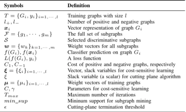
1 10 100 1000 10000 100000 100 500 1000 10000 20000 25000 Time (Seconds)
No. of Training Graphs Time Complexity with Different No. of Training Graphs
igBoost gBoost
Fig. 1: Training timew.r.t. different number of graphs on NCI-1 dataset for gBoost [5] and igBoost algorithm [11]. Runtime of existing graph classification algorithms exponentially growsw.r.t.the increase of the training set size.
to computer servers, leading to severe security issues in our social life, such as private information leak or internet breakdown. Therefore, misclassification of a malicious traf-fic (graph) would have a much higher economic and social costs in terms of its potential impacts.
Motivated by its significance in practice, cost-sensitive learning has established itself as an active topic in data min-ing and machine learnmin-ing areas [14], [15], [16], [17], [18], [19], [20], [21], [22], [23], [24] in the last decade. Common solutions to cost-sensitive problem includes sampling [19], decision tree modelling [25], [17], boosting [20], [21], and SVM adaptations [15], [22], [26]. However, all these methods are only dedicated to generic datasets with feature-vector representation, whereas graphs do not have features immediately available and only contain nodes and their dependency structure information. Simply enumerating sub-graph structures as features is clearly a suboptimal solution for cost-sensitive learning, mainly because substructure space is potentially infinite and we need a good strategy to find high quality features to help avoid misclassifications on positive classes.
Recently, an igBoost [11] algorithm has been proposed to handle imbalanced graph datasets. The igBoost approach, extended from a standard cost-insensitive graph classifica-tion algorithm gBoost [5], assigns proper weight values to different classes by taking data imbalance into consider-ation, so the algorithm is potentially useful to tackle the cost-sensitive learning problem for graphs. However, the loss function defined in igBoost is not cost-sensitive but only aims to minimize the misclassification errors. As a result, if the training data are separable [22], the algorithm will have limited power to enforce the cost-sensitivity learning because it only tries to separate training samples without using costs associated to different classes to tune the decisions for minimum costs. From a statistical point of view, the minimum risk could be achieved by following Bayes decision rules to predict graph samples. The objec-tive functions in [11] is non-optimal because it simply employs some heuristic schemes, rather than implements the Bayes decision rules to minimize the conditional risk for cost-sensitive setting. In other words, the current boosting style algorithms are not targeting cost-sensitive learning problems for graph data.
1.2 Fast Training for Large Scale Graphs
Another challenge of existing graph classification algo-rithms is that they are only designed for small size graph datasets and are very inefficient to scale up to large size graph datasets. Taking existing boosting-based graph classification algorithms [11], [5] as examples, a boosting algorithm iteratively selects the most discriminative sub-graphs from the graph dataset and then solves a linear programming problem for graph classification. In practice, although one may use an appropriate support value in the first step to find subgraphs, by using subgraph mining based algorithm such as gSpan [27], the linear programming solving in each iteration in the second step is a very time-consuming process, which prevents the algorithms from scaling up to large scale graph datasets.
In Fig. 1, we report the runtime of boosting-based graph classification algorithms with respect to different numbers of training graphs. For a small number of graphs,e.g.100 to 1000, both gBoost [5] and igBoost [11] are relatively efficient (requiring 5 to 300 seconds for training). However, when the number of training graphs is considerably large (25,000 graphs or more), the training time for both gBoost and igBoost increase dramatically (about 50,000 seconds), and requires over 13 hours to complete the training task. As big data applications [28] are becoming increasingly popular for different domains and result in graph datasets with large volumes, finding effective boosting algorithms for large scale graph datasets is highly desired.
If we consider both cost-sensitive learning and fast graph classification as a whole, the following issues should be taken into consideration to ensure the efficiency and the effectiveness of the algorithm:
1) Cost-Sensitive Subgraph Selection:In a cost-sensitive setting, we are given a cost matrix representing misclassification costs. To ensure minimum costs for graph classification, we should take cost of individual samples into consideration to cost-sensitively select discriminative subgraphs. A cost-sensitive subgraph exploration process is, therefore, essential, but has not been addressed by existing research.
2) Model Learning for Cost-Sensitivity: For existing boosting-based graph classification algorithms, they all have non-optimal loss function, and therefore have limited capability to handle cost-sensitive problems. Alternatively, we should employ a proper loss func-tion, which not only implements the cost-sensitive Bayes decision rule, but also approximates the Bayes risk. By doing this, the induced model will have max-imum power for cost-sensitive graph classification. 3) Fast Training on Large Graph Datasets: All
boost-ing algorithms are difficult to scale to large graphs because the optimization procedures involved in each iteration needs to resolve a large scale linear program-ming problem, which is typically time-consuprogram-ming. We need new optimization techniques to enable fast training on large scale graph datasets.
paper, CogBoost, a fast cost-sensitive learning algorithm for graph classification. Instead of simply assigning weights to different classes, we derive a loss function which im-plements the Bayes decision rule and guarantees minimum risk for prediction. To identify discriminative subgraphs for cost-sensitive graph classification, we consider individual cost of each graph sample, which is completely model driven, i.e., we progressively select the most informative subgraphs based on current learned model, and the newly selected subgraph is added to current feature set to refine the classifier model. These two steps are mutually beneficial to each other. To enable fast training on large graph datasets, an advanced optimization technique,cutting plane algorithm, is derived to solving linear program efficiently. Experiments on real-word large graph datasets demonstrate CogBoost’s perofrmance.
The remainder of the paper is structured as follow. Section 2 reviews related work. The problem definition and overall framework are discussed in Section 3. Section 4 reports our CogBoost algorithm for cost-sensitive graph classification. The cutting plane algorithm for fast training is reported in Section 5, followed by the time complexity analysis in Section 6. The experiments are reported in Section 7, and we conclude the paper in Section 8.
2
RELATED WORK
Our work is closely related to graph classification and cost-sensitive learning.
Graph Classification Learning and classifying graph data have drawn much attention in recent years. Because graphs involve node-edge structures whereas most existing classi-fication methods use instance-feature representation model, the major challenge of graph classification is to transfer graphs into proper format for learning methods to train classifiers. Existing methods in the area mainly fall into two categories: (1) global similarity-based approaches [1], [4]; and (2) local subgraph based approaches [5], [7], [8]. For global similarity-based methods, graph kernels and graph embedding are used to calculate the distance between a pair of graphs, and the distance matrix can be fed into a learning algorithm, such ask-NN and SVM, for graph classification. For subgraph feature based methods, the major goal is to identify significant subgraphs which can be used as signature for different classes [7], [29], [5], [9], [30]. By using subgraph features selected from the graph set, one can easily transfer graphs into a vector space so existing machine learning methods can be applied for classifica-tion [7], [29]. In [31], the authors propose a structure feature selection method to consider subgraph structural information for classification. Jin [32] proposes to extract subgraph patterns and use their co-occurrence to build classifier for graph classification. Other method [33] regards subgraph selection as combinatorial optimization problem and uses heuristic rules, in combination with frequent subgraph mining algorithm such as gSpan [27], to find subgraph features.
After obtaining subgraph features, one can also employ Boosting algorithms for graph classification [34], [5], [9],
[35]. In [9], the authors proposed to boost the subgraph decision stumps from frequent subgraphs, which means they first need to provide a minimum support to mine a set of frequent subgraphs and then utilize the function space knowledge for boosting. In contrast, gBoost [34] and its variants [5], [11] do not require a minimum support, the pruning search space relies on the effective rules derived by the authors. gBoost adopts an Adaboost procedure in [34], and it is formalized as a mathematical margin maximization problem in its latter variant [5]. The mathematical LP-boost style of algorithm in [5] demonstrated that the method is effective and converges very fast.
The above algorithms, regardless of whether they transfer graphs into a feature space or boosting directly from the weak subgraph decision stumps, are designed for cost-insensitivity scenarios, i.e., they assume that all misclas-sifications are subject to the same cost/risk. Recently, an igBoost [11] algorithm has been proposed to deal with imbalanced graph datasets (we extend igBoost to handle dynamic data streams in [36]). igBoost assigns different weight values to different classes in order to combat class imbalance issue, which can deal with cost-sensitive problem to some extend. However, the loss function of igBoost is rather heuristic and cannot guarantee the minimization of the misclassification costs. In another words, igBoost is a sub-optimal solution to deal with cost-sensitive graph classification.
Cost-sensitive Learning Cost-sensitive learning has been extensively studied in the last decade. Approaches for cost-sensitive learning can be mainly distinguished into the following four categories: (1) Sampling methods [19]; (2) Decision tree approaches [25], [17]; (3) Boosting algo-rithms [37], [20], [21]; and (4) SVM adaptation [15], [22]. Sampling approaches [19] aim to re-weight the training samples proportional to their cost values, which can be done by over-sampling, or cost-proportionate rejection sampling. The main goal is to change the sample distributions so that any classifier can be directly used to handle cost-sensitive problems. Decision tree modelling approaches [25], [17] incorporate the costs during the tree construction, so that misclassification cost at the leaves is minimized. Boosting algorithms [37], [20], [21], such as AdaCost [37], use the misclassification costs to update the training distributions on successive boosting rounds, which has been proved to be effective to reduce the upper bound of cumulative misclassi-fication cost of the training set. SVM adaptation [15], [22] represents a set of approaches based on SVM adaptation for cost-sensitive learning. They either shift the decision boundaries by simply adjusting the threshold of standard SVMs [26] or introduces different penalty factorsC1 and C−1 for the positive and negative SVM slack variables during training [15]. Recently a CS-SVM algorithm [22] is proposed which utilizes an optimal hinge loss function. It is shown in [22] that CS-SVM outperforms previous approaches [15], [26].
In summary, the scope of all existing cost-sensitive methods is limited to data in vector format. In this paper, we consider the unique challenges of graph data, and propose
a novel algorithm for cost-sensitive graph classification.
3
PROBLEM
DEFINITION
ANDOVERALL
FRAMEWORK
Definition1: Connected Graph: A graph is denoted
as G = (V, E,L), where V = {v1,· · · , vnv} is a set of
vertices,E⊆ V × V is a set of edges, and Lis a labeling function assigning labels to a node or an edge. A connected graph is a graph such that there is a path between any pair of vertices.
In this paper, each labeled graphGiis a connected graph
with a class label yi ∈ Y ={−1,+1}, i.e., we consider
binary classification. Ifyi= +1,Gi is a positive graph, or
negative otherwise.
Definition2: Subgraph: Given two connected graphs
G= (V, E,L) andgi = (V0, E0,L0),gi is a subgraph of
G(i.egi⊆G) if there is an injective functionfb:V0→ V,
such that∀(a, b)∈E0, we have(fb(a),fb(b))∈E,L0(a) = L(fb(a)), L0(b) = L(fb(b)), L0(a, b) = L(fb(a),fb(b)). If
gi is a subgraph of G (gi ⊆G), Gis a supergraph of gi
(G⊇gi).
Classifier Model for Graphs: A classifier model f(·),
which is learned from a set of training graphs T = {(G1, y1),· · ·,(Gl, yl)}, is a function to map a connected
graphGi from graph spaceG (Gi ∈ G) to the label space Y = {+1,−1}. For cost-sensitive learning, the classifier f(·)is required to minimize the expected misclassification cost/riskR=EGi,yi[L(f(Gi), yi)], whereL(f(Gi), yi)is
a non-negative loss function with respect to the misclassi-fication cost. A typical loss function is as follows:
L(f(Gi), yi) = 0 : f(Gi) =yi C1 : f(Gi) =−1, yi= 1 C−1 : f(Gi) = 1, yi=−1 (1)
The loss function in Eq. (1) is extended from the standard 0-1 loss function, i.e., L(f(·), y) = I(f(·) 6= y), where I(·) is an indicator function, I(a) = 1 if a holds, or I(a) = 0 otherwise. In Eq. (1), when C1=C−1= 1, the function L(f(Gi), yi)) is cost-insensitive and degenerates
to the standard 0-1 loss. For cost-sensitive learning, a false negative (f(Gi) = −1, yi = 1) prediction usually incurs
a larger cost than a false positive (f(Gi) = 1, yi = −1)
prediction, i.e.,C1> C−1.
Given a set of training graphs T =
{(G1, y1),· · ·,(Gl, yl)}, and C1 and C−1 for the cost of misclassification, cost-sensitive graph classification
aims to build an optimal classification model f(·) from T to minimize the expected misclassification loss (also known as risk)R=EGi,yi[L(f(Gi), yi)]. Some important
notations used in the paper are listed in Table 1. 3.1 Overall Framework
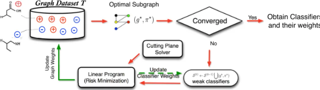
In this paper, we propose a boosting framework for cost-sensitive graph classification. Our framework (Fig. 2) mainly consists of three steps.
1) Optimal Subgraph Exploration: One optimal sub-graph is selected each step, and the cost-sensitive
TABLE 1: Important notations used in the paper
Symbols Definition
T={Gi, yi}i=1,···,l Training graphs with sizel
l+, l− Number of positive and negative graphs xi Vector representation of graphGi
F={g1,· · ·, gm} The full set of subgraphs
S Selected discriminative subgraphs
w={wk}k=1,···,m Weight vectors for all subgraphs
f(Gi), f(xi) Classifier prediction on graphGi
L(f(Gi), yi) A loss function
C1, C−1 Cost of positive and negative graphs, respectively ξ={ξi}i=1,···,l Vector, slack variables for cost-sensitive learning
ξ Slack variable (a scalar) for cutting plane algorithm
µ={µi}i=1,···,l Weight vectors of training graphs
C, γ Parameters for cost-sensitive learning
Tmax Maximum number of iterations
min sup Mininum support for subgraph mining
Cutting-plane termination threshold
discriminative subgraph exploration is guided by the model learnt from the previous step. The newly ex-tracted subgraph is added to the most discriminative setS to enhance the learning in the next step. 2) Risk Minimization and Fast Training: A linear
pro-gram is solved to achieve minimum risk based on current selected subgraphs. To enable fast training on large scale graphs, a novel cutting plane algorithm is employed.
3) Updating Graph Weights for New Iteration:After the linear program is solved, the weight values for train-ing graphs are updated and the algorithm continues in a new iteration until the whole algorithm converges. Next we will present our Cogboost algorithm for cost-sensitive graph classification and then propose a cutting plane algorithm to handle large scale graph datasets.
4
COST-SENSITIVE
LEARNING FOR
GRAPH
DATA
For graph classification, boosting [5][11] has been previ-ously used to identify subgraphs from the training graphs as features. After that, each subgraph is regarded as a decision stump (weak classifier) to build a boosting process:
~gk(Gi;πk) =πk(2I(gk ⊆Gi)−1); (2)
whereπk ∈ Y ={−1,+1} is a parameter controlling the
label of the classifier. In this paper, the weak classifier is written as~gk(Gi)for short.
Let F = {g1,· · ·, gm} be the full set of subgraphs in
T. We can use F as features to represent each graph Gi
into a vector space asxi={~g1(Gi),· · ·,~gm(Gi)}, with
xki =~gk(Gi). In the following subsection, we useGi and
xi interchangeably as they are both refereed to the same
graph.
The prediction rule for a graphGiis a linear combination
of the weak classifiers: f(xi) =wTxi=
X
(gk,πk)∈F ×Y
wk~gk(Gi) (3)
wherew={wk}k=1,···,mis the weight vector for all weak
classifiers. The predicted class label ofxi is +1 (positive)
+ +
-Graph Dataset T Optimal Subgraph
Converged weak classifiers Linear Program (Risk Minimization) Update Graph W eights Update Classifier Weights Obtain Classifiers and their weights Yes No Cutting Plane Solver -- + +
-Fig. 2:The proposed fast cost-sensitive boosting for graph classification framework. In each iteration, CogBoost selects an optimal subgraph feature(g?, π?)based on
current learned model and weights of training graphs. Then(g?, π?)is added to the current selected setS. Afterwards, CogBoost solves a linear programming problem
to achieve cost/risk minimization. To enable fast training on large scale graph datasets, a cutting plane solver is used in this step to improve the algorithm efficiency. After solving the linear program, two sets of weights (green arrows) are updated: (1) weights for training graphs, and (2) weights for weak learners (subgraphs). The feature selection and risk minimization procedures continue until CogBoost converges or reaches the predefined number of iterations.
Similar to SVM, gBoost [5] aims to achieve minimum loss w.r.t. a standard hinge loss function L(f, y) = b1−
yfc+, where bxc+ = max(x,0). igBoost [11] extends gBoost by assigning larger weight values to graphs in different classes. Both gBoost and igBoost are not optimal when dealing with cost-sensitive cases, because their loss functions do not follow the Bayes decision rules to min-imize the expected risk/loss. In this section, we will first present an optimal hinge loss function, and then formalize our algorithm into a boosting paradigm.
4.1 Optimal Cost-sensitive Loss Function
A graph classifier f(·) maps a graph Gi to a class label
yi ∈ {−1,1}. Assume graphs and class labels are drawn
from probability distribution PG(Gi) andPY(yi),
respec-tively. Given a non-negative loss function L(f(Gi), yi),
the classifierf(Gi)is optimal if it minimizes the loss/risk
R = EGi,yi[L(f(Gi), yi)]. Let η = PY|G(1|Gi) be the
probability forGibeing 1, from a Bayes decision rule point
of view, this is equivalent to minimize the conditional risk. EY|G(L(f(Gi), yi)|G=Gi) =ηL(f(Gi),1)
+(1−η)L(f(Gi),−1)
(4) The loss function in Eq. (1) is a Bayes consistent loss function [38],i.e., it implements the Bayes decision rule to achieve minimum conditional risk (Eq. (4)). This suggests that ideally Eq. (1) can be used to design some cost-sensitive algorithms for minimizing conditional risk. How-ever, Eq. (1) is extended by a 0-1 loss function. Minimizing the 0-1 loss is computationally expensive because it is not convex. State of the art algorithms usually use surrogate loss functions to approximate the 0-1 loss (e.g., SVM and gBoost [5] employ hinge loss). The hinge loss induced SVM algorithms enforces maximum margins between the support vectors and the hyper-planes, which can achieve good classification performance.
A recent work on SVM [22] theoretically suggests that the standard hinge loss can be extended to be cost-sensitive, by setting the loss functionL(f(Gi), yi) as follows:
L(f(Gi), yi) =
bC1−C1·f(Gi)c+ : yi= 1 b1 + (2C−1−1)·f(Gi)c+ : yi=−1
(5)
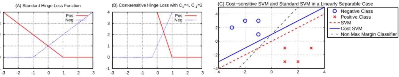
It is proved in [22] that the new hinge loss function Eq. (5) also implements the Bayes decision rule. Additionally, employing Eq. (5) also enjoys the merit of maximum margin principal for classification. The standard hinge loss and its cost-sensitive hinge loss is illustrated in Fig. 3. They have different explanations with respect to the loss and the margins (distance to the hyperplane from support vectors). Specifically, for standard hinge loss (Fig. 3. (A)), the positive and negative class both have equal margins (unit margins); and for cost-sensitive hinge loss (Fig. 3. (B) ), the negative class has a much smaller margin when the positive class still have a unit margin. As shown in Fig. 3. (C), the margins for positive and negative classes are uneven when cost-sensitive hinge loss function Eq. (5) is utilized in a SVM formulation.
Note that the loss function employed in igBoost [11] is heuristically adapted from standard hinge loss, which does not necessarily follow the Bayes decision rule. In other words, it is a sub-optimal loss function for cost-sensitive learning. In the following subsection, we will use the cost-sensitive hinge loss function in Eq. (5), and re-formulate it into a linear program boosting framework.
4.2 Cost-Sensitive Formulation for Graphs Motivated by the optimal loss function in Eq. (5), we formalize our learning task as the following regularized risk minimization problem: min w kwk+ C l{ P {i|yi=1} L(f(xi),1) + P {j|yj=−1} L(f(xj),−1)} s.t. w0 (6) In Eq.(6), we enforce the weight for each subgraph to be positive,i.e.,w0. We also impose 1-norm regularization on w (i.e., kwk), which will favor sparse solutions with many variables being exactly 0. This strategy is similar to the problem of LASSO for variable shrinking [39]. And we use i and j to index the positive and negative training graphs, respectively. C is a parameter to trade-off the regularization term and loss term. The objective
-1 0 1 2 3 4 -3 -2 -1 0 1 2 3 (A) Standard Hinge Loss Function
Pos Neg -1 0 1 2 3 4 -3 -2 -1 0 1 2 3 (B) Cost-sensitive Hinge Loss with C1=4, C-1=2
Pos Neg −4 −2 0 2 4 −4 −2 0 2 4
(C) Cost−sensitive SVM and Standard SVM in a Linearly Separable Case Negative Class Positive Class SVM Cost SVM
Non Max Margin Classifier
Fig. 3:Different loss functions and formulations with respect to support vector machines (SVMs): (A) Standard Hinge Loss, (B) Cost-sensitive Hinge Loss withC1= 4
andC−1= 2, and (C) Different SVM formulations with Standard Hinge Loss and Cost-sensitive Hinge Loss (cf.[22]).
function in Eq.(6) can be reformulated as follows:
min w,ξ kwk+ C l{C1 P {i|yi=1} ξi+γ P {j|yj=−1} ξj} s. t. f(xi)≥1−ξi, yi= 1 f(xj)≤ −1γ +ξj, yj=−1 f(xi) = m P k=1 wk·~gk(Gi) w0,ξ0, γ= 2C−1−1, (7)
In Eq.(7), ξi and ξj are slack variables concerning the
loss of misclassifying a positive and a negative graph, respectively. In this case, cost-sensitivity is controlled by C1 and γ, which impose a smaller margin on negative examples than positive examples (In Fig. 3. (B) and (C), for an example withC1= 4, andγ= 2C−1−1 = 3, the margin for negative example is 1γ = 1
3). As suggested in [38], we can setγas a parameter subject to1≤γ≤C1 instead of a fixed value (2C−1−1) to achieve better classification.
Solving objective function in Eq. (7) requires a com-plete set of subgraph features (i.e., represent Gi as xi = {~g1(Gi),· · ·,~gm(Gi)}), which are unavailable unless we
enumerate the whole subgraph space in advance. In prac-tice, this is likely impossible because the whole subgraph set is very large and possibly infinite. In the following subsection, we will transfer this formulation to its Lagrange dual problem and use a boosting algorithm to solve it in an iterative way.
4.3 Boosting for Cost-sensitive Learning on Graphs
The Lagrange dual of a problem usually provides additional insights to the original (primal) problem. The dual problem of Eq.(7) is1 max µ Pl+ i=1µi+1γP l− j=1µj s.t. l+ P i=1 µi~gk(Gi)− l− P j=1 µj~gk(Gj)≤1,∀gk∈ F 0≤µi≤ CCl−1, i= 1,· · · , l+ 0≤µj≤ γCl , j= 1,· · · , l− (8) wherel+andl−indicate the number of graphs in positive
and negative sets (l=l++l−), respectively. While solving
the primal problem in Eq.(7) returns a vectorw indicating 1. The derivation from the primal problem Eq.(7) to dual problem Eq.(8) is shown in Appendix A.1.
the weights of each subgraphs, the dual problem in Eq. (8) will produce a vectorµ= {µi}i=1,···,l. Nevertheless,
Eq.(7) and Eq.(8) will generate the same objective values.
Insights of Dual Problem (1) The solution {µi}i=1,···,l
can be interpreted as the weight values of graphs in order to achieve minimum loss. (2) Each constraint
Pl+
i=1µihgk(Gi)−
Pl−
j=1µjhgk(Gj)≤1 in Eq. (8)
indi-cates a subgraph patterngk over the whole training graphs.
It provides a natural metric to assess the cost-sensitive discriminative power of a subgraph.
Definition3: Cost-sensitive Discriminative Score:For
a subgraph decision stump~gk(Gi), its cost-sensitive
dis-criminative score over the whole training graphs is:
Θ(gk, πk) = l+ X i=1 µi~gk(Gi)− l− X j=1 µj~gk(Gj) (9)
Eq.(8) requires discriminative scores for all subgraphs
≤1, which latter will serve as an termination condition of our iterative algorithm.
Linear Program Boosting Framework Because we do
not have a predefined feature setF in advance, we cannot solve Eq.(7) or Eq.(8). Therefore, we propose to usecolumn generation (CG) techniques [40] to solve the objective function (Eq. (7)). The idea of CG is to begin with an empty feature set S, and iteratively select and add one feature/column to S which violates the constraint in the dual problem (Eq. (8)) mostly. AfterS is updated, CG re-solve the primal problem Eq.(7). This procedure continues until no more subgraph violating the constraint in (Eq.(8)). Our cost-sensitive graph boosting framework is illus-trated in Algorithm 1. CogBoost iteratively selects the most discriminative subgraph(g?, π?)at each round (step 4). If
the current optimal pattern no longer violates the constraint or it has reached the maximum number of iterationsTmax,
the iteration process stops (steps 5-6). Because in the last few iterations, the optimal value only changes subtlety, we add a small value ∆ to relax the stopping condition (typically, we use∆ = 0.01 in our experiments). In step 8, we solve the linear programming problem based on the selected subgraphs to recalculate two set of weights: (1) w(t), the weights for subgraph decision stumps inS; and (2)µ(t), the weights of training graph for optimal subgraph mining in the next round, which can be obtained from the Lagrange multipliers of the primal problem. Once the algorithm converges or the number of maximum iteration is
Algorithm 1 CogBoost Algorithm for Graph Classification Require:
Tl={(G1, y1),· · ·,(Gl, yl)}: Training Graphs;
Tmax: Maximum number of iteration;
Ensure: f(xi) =P (gk,πk)∈Sw (t−1) k ~gk(Gi): Classifier; 1: S ← ∅; 2: t←0; 3: whiletruedo
4: Obtain the most discriminative decision stump(g?, π?);
//Al-gorithm 2; 5: ifΘ(g?, π?)≤1 + ∆ or t=T maxthen 6: break; 7: S ← SS (g?, π?);
8: Solve Eq. (7) based onSto getw(t), and Lagrange multipliers
of Eq. (8)µ(t); 9: t←t+ 1; 10: return f(xi) =P (gk,πk)∈Sw (t−1) k ~gk(Gi);
Algorithm 2 Cost-sensitive Subgraph Exploration
Require:
Tl={(G1, y1),· · ·,(Gl, yl)}: Labeled Graphs;
µ={µ1,· · ·, µl}: Weights for labeled graph examples;
min sup: mininum support for subgraph mining;
Ensure:
(g?, π?): The most discriminative subgraph;
1: τ= 0,(g?, π?)← ∅;
2: whileRecursively visit the DFS Code Tree in gSpando 3: gp←current visited subgraph in DFS Code Tree;
4: ifgphas been examinedorsup(gp)< min supthen
5: continue;
6: Compute scoreΘ(gp, πp)for subgraphgpaccording Eq.(9);
7: ifΘ(gp, πp)> τ then
8: (g?, π?)←(g
p, πp); τ←Θ(gp, πp);
9: if The upperbound of scoreΘ(b gp)> τ then
10: Depth-first search the subtree rooted from nodegp;
11: return (g?, π?);
reached, CogBoost returns the final classifier modelf(xi)
in step 10.
4.4 Cost-sensitive Subgraph Exploration
To learn the classification model, we need to find the most discriminative subgraph which considers each training graph’s weight in each step (step 4 in Algorithm 1). The subgraph exploration is completely model driven,i.e., we select a subgraph which violates the constraint in Eq.(8) mostly. Based on the definition of discriminative score in Eq.(9), we need to perform a weighted subgraph mining over training graphs.
In CogBoost, we employ a Depth-First-Search (DFS) based algorithm gSpan [27] to enumerate subgraphs. The key idea of gSpan is that each subgraph has a unique DFS Code, which is defined by its lexicographic order of the discovery time during the search process. Two subgraphs are isomorphism iff they have the same minimum DFS Code. By employing a depth first search strategy on the DFS Code tree (where each node is a subgraph), gSpan can enumerate all frequent subgraphs efficiently. To speed up the enumeration, we further employ a branch-and-bound scheme to prune the search space of DFS Code tree by utilizing an upper bound of discriminative score [5] for each subgraph pattern.
Our subgraph mining algorithm is listed in Algorithm 2. The minimum value τ and optimal subgraph (g?, π?)
are initialized in step 1. We prune out duplicated subgraph features or subgraph with low support (sup(·) returns the support of a subgraph) in step 4-5, and compute the discriminative scoreΘ(gp, πp)forgpin step 6. IfΘ(gp, πp)
is larger thanτ, we update the optimal subgraph in step 8. We use an branch-and-bound pruning rule in [5] to prune the search space in steps 9-10. Finally, the optimal subgraph pattern(g?, π?)is returned in step 11.
5
F
ASTT
RAINING FORL
ARGES
CALEG
RAPHSFor CogBoost algorithm, it needs to iteratively mine an optimal subgraph (step 4 of Algorithm 1) and solve a linear problem (step 8 of Algorithm 1). To enable fast training for large scale graph datasets, for step 4 we can set a proper support and use some heuristic techniques, such as reusing the search space during the enumeration of subgraphs rather than re-mining subgraph from scratch, just as [5] does. For step 8, in this section, we derive acutting planealgorithm to speed up the training process.
5.1 Froml-Slacks to 1-Slack Formulation
Eq.(7) in step 8 of Algorithm 1 has l = l+ +l− slack
variablesξi andξj, inspired by the techniques used in the
SVM formulation [41], we propose to solve it efficiently by reducing the number of slack variables as follows,
min w,ξ kwk+Cξ s. t. ∀c∈ {0,1}l, 1 lw T{C 1 P yi=1 cixi−γ P yj=−1 cjxj} ≥1 l{C1 P yi=1 ci+ P yj=1 cj} −ξ, w0, ξ≥0. (10) The above formulation only has one slack variable ξ, which can be proved to be equal to Eq.(7) 2, with ξ={C1 P
{i|yi=1}
ξi+γ P
{j|yj=−1}
ξj}/l. Note that although
Eq.(10) has2l constraints in total, such a formulation can
be solved by cutting plane algorithm in a linear time by iteratively selecting a small number of most violated con-straints (Cutting Planes). This leads to an efficient solution to the optimization, so our algorithm can effectively scale to large datasets.
The dual ofl-slack formulation in Eq.(8) provides solu-tionµwhich can interpret the graph weights for subgraph mining in the next iteration. To establish the same relation-ship between the new objective function Eq.(10) and the graph weightsµ, we also refer to its dual problem, which is given as follows3: max λc c1 l P c λcP i ci+1lP c λcP i cj s.t. C1 l P c λcP i cixki − γ l P c λcP j cjxkj ≤1,∀k 0≤P c λc≤C. (11)
2. Appendix A.2 proves the equality of Eq.(7) and Eq.(10). 3. The derivation from Eq.(10) to Eq.(11) is given in Appendix A.3.
Comparing the the dual problems of Eq.(8) and Eq.(11), they are identical if:
µi|yi=1= C1 l X c λcci; µj|yj=−1= γ l X c λccj; (12)
5.2 Cutting-plane Algorithm for Fast Training The basic idea of cutting-plane algorithm is similar to the column generation algorithm, or it can be regarded as a row generation algorithm (each constrain in Eq.(11) is a row). Instead of considering all constrains (rows) as a whole, our cutting-plane algorithm considers only the most violated constraint (row) each time. The selected violated constraints form a working setW. And it utilizes an iterative procedure to solve the problem. By doing this, the linear program can be solve efficiently.
Our detailed cutting plane algorithm is shown in Algo-rithm 3. Initially, the working set W is an empty set in step 1. In each iteration, we solve the optimization problem based on current working setW in step 3 (w=0 andξ= 0
for the first iteration). Steps 4-6 find the most violated constraint, which is determined by the cost-sensitive loss function in Eq.(5). Step 9 adds the current most constraint to the working set. The iteration continues until it reaches the convergence (steps 7-8). Also, we add a small constant (In our experiments, we set= 0.01as default value) to enable early termination of iterations.
Our cutting plane algorithm can always return an -tolerance accurate solution (approximate the solution of Eq. (7) very well). It is efficient because each time we solve a linear program in a small working set, the cutting plan algorithm is independent of the number of sample size. This essentially ensures that our solutions can scale to very large scale graph datasets.
6
T
IMEC
OMPLEXITYA
NALYSIS: T
HEORET-ICAL
A
SPECT ANDP
RACTICEThe time complexity of CogBoost includes two major components: (1) mining a cost-sensitive discriminative sub-graphs O(P(l)) (step 4 of Algorithm 1), and (2) solving a linear program problem O(Q(l)) (step 8 of Algorithm 1), where P and Q are functions for mining subgraph and solving LP problem of size l. For subgraph mining, CogBoost employs a gSpan based algorithm (Algorithm 2) for subgraph enumeration in the first iteration (O(P(l))), and re-uses the search space [5] of the first iteration (O(P(l))). Because re-using search space can significantly reduce the mining time, we have O(P(l)) O(P(l)). Suppose the number of iterations of CogBoost (Algorithm 1) isTmax, the total time complexity of CogBoost is:
O=O(P(l)) + (Tmax−1)O(P(l)) +TmaxO(Q(l)) (13)
6.1 Time complexity of Subgraph Mining
Theoretical Aspect: Intuitively, because the subgraph
space is infinitely large, the time complexity for subgraph
Algorithm 3Cutting plane algorithm for linear problem Eq.(7) Require:
{x1,· · ·,xl}: Training graphs with subgraph representation.
C, C1, C−1: Parameters for classifier learning.
: Cutting-plane termination threshold. Ensure:
w: Classifier weights; µ: Graph weights; 1: InitializeW ← ∅;
2: whiletruedo
3: Obtain primal and dual solutionsw, ξ,λby solving
min w,ξ kwk+Cξ s. t. ∀c∈ W, wT1 l{C1 P yi=+1 cixi−γ P yj=−1 cjxi} ≥ 1 l(C1 P yj=1 ci+ P yi=−1 cj) +ξ, w0, ξ >0. 4: fori= 1· · ·ldo
5: applying the following rule the find the most constraint variables on positive graphs (yi= 1)
ci=
1 : yi·f(xi)<1
0 : else
6: applying the following rule to negative graphs(yj=−1)
cj= 1 : γ·yi·f(xi)<1 0 : else 7: if 1l(C1 P yi=1 ci + P yj=−1 cj) − wT1 l(C1 P yi=+1 cixi − γ P yj=−1 cjxi)≤ξ+then 8: break; 9: W ← WS c;
10: updateµiandµjaccording to Eq. (12);
11: return wandµ;
mining is NP-hard, andO(P(l))for subgraph mining is in-evitable for graph classification. Thus all existing subgraph feature selection algorithms for graph classification [5], [7], [33] derive some upper-bounds to prune the search space. In CogBoost, we incorporate the upper-bound in [5] and the support thresholdmin supto reduce the sugraph space. It is worth noting that CogBoost can still function property even though users do not specify the min sup value for subgraph mining. Ifmin supwere not specified, CogBoost will only rely on the upper-bound in [5] to prune the search space.
Practice: In practice, we observe that when the data set is considerable large (e.g., 40,000 chemical compounds or more), setting a support threshold min sup = 5%
can significantly speed up the mining progress. However, setting a threshold may incur missing of discriminative sub-graphs because some infrequent subsub-graphs are not checked. Accordingly, we suggest removing themin supthreshold for small graph dataset while setting a proper support for large datasets. The proper support value depends on the domains of applications. For instance, when the average number of nodes and edges of the graph dataset are large, a larger support (5-10%) is preferred. On the other hand, if the average number of nodes and edges are small, a small support (about 1%-3%) is a good choice. For real-world applications, it is useful to first check the statistics of the graph samples before carrying out the graph classification tasks.
TABLE 2: Graph Datasets Used in the Experiments
Datasets #Pos #Total #Nodes #Edges Descriptions NCI-1 1,793 37,349 26 28 Lung Cancer NCI-33 1,467 37,022 26 28 Melanoma NCI-41 1,350 25,336 27 29 Prostate Cancer NCI-47 1,735 37,298 26 28 Central Nerve NCI-81 2,081 37,549 26 28 Colon Cancer NCI-83 1,959 25,550 27 29 Breast Cancer NCI-109 1,773 37,518 26 28 Ovarian NCI-123 2,715 36,903 26 28 Leukemia NCI-145 1,641 37,041 26 28 Renal Cancer
Twitter 66,458 140,949 4 5 Sentiment
6.2 Time complexity of LP Solving
Theoretical Aspect: For LP problem solving, Eq. (7)
is solvable in polynomial time O(Q(l)) = O(lk) with some constant k [42]. In other words, gBoost [5] and igBoost [11] needs polynomial time for this step. By using cutting plane algorithm, the time complexity would be O(Q(l)) = O(sl), where s is the number of non-zeros features in the original problem (please refer to [41] for detailed analysis). Therefore, CogBoost can significantly reduce the runtime when the graph sample sizelis large. In Section 7, our experiments will soon demonstrate that the improvement of LP problem solving without using cutting plan algorithm is marginal.
Practice: The cutting plane algorithm uses a working set
W (in Algorithm 3),W overlaps significantly during two consecutive iteration of Algorithm 1. Therefore, in our im-plementations, we re-use top 200 most violated constrains in W in the previous iteration, which can significantly improve the algorithm efficiency. In practice, the classifier weightsw in two consecutive iterations may be very close to each other, one can also use the warm-start technique (using w in previous iteration as initial value for linear problem solving) to speed up the learning process.
7
E
XPERIMENTSIn this section, we evaluate CogBoost in terms of its average misclassification cost (or average cost) and runtime performance. The average costis calculated by using the total misclassification costs divided by the number of test instances. The lower the average costs, the better the algo-rithm performance is. The runtime performance is evaluated based on the actual runtime of the algorithm.
7.1 Experimental Settings
Two types of real-life datasets, NCI chemical compounds and Twitter graphs, are used in our experiments. Table 2 summaries the statistics of the two benchmark datasets.
NCI Graph Datasetsare commonly used as the benchmark
for graph classification. In our experiments, we download nine NCI datasets from PubChem 4. Each NCI dataset belongs to a bioassay task for anticancer activity prediction, where each chemical compound is represented as a graph,
4. http://pubchem.ncbi.nlm.nih.gov
with atoms representing nodes and bonds as edges. A chemical compound is positive if it is active against the corresponding cancer, or negative otherwise.
Table 2 summarizes the NCI graph data used in our experiments. We have removed disconnected graphs and graphs with unexpected atoms (some graphs have atoms represented as ‘*‘) in the original graphs. Columns 2-3 show the the number of positive and total number of graphs in each dataset, and Columns 4-5 indicate the average number of nodes and edges in each dataset, respectively.
Stanford Twitter Graphsare extracted from twitter
sen-timent classification5. Because of the inherently short and sparse nature, twitter sentiment analysis (i.e., predicting whether a tweet reflects a positive or a negative feeling) is a difficult task. To build a graph dataset, we represent each tweet as a graph by using tweet content, with nodes in each graph denoting the terms and/or smiley symbols (e.g, :-D and :-P) and edges indicating the co-occurrence relationship between two words or symbols in each tweet. To ensure the quality of the graph, we only use tweets containing 20 or more words. In our experiments, we use tweets from April 6 to June 16 to generate 140,949 graphs (in a chronological order). Note that this dataset has been used for simulated graph stream classification in our previous study [36]. In this paper, we aggregate all graphs as one dataset without considering their temporal order.
Baselines We compare our proposed CogBoost algorithm
with the following baseline algorithms.
• gBoost[5] is a state-of-the-art boosting method, which has demonstrated good performance for graph classi-fication.
• igBoost [11] extends gBoost to handle imbalanced
graph datasets. The weight of a minority (positive) graph is assigned with aβ times higher weight value than a majority (negative) graph.
• Fre+CSVM first mines a set of frequent subgraphs
(with minimum support 3%) from the entire graph dataset, and selects the top-Kmost frequent subgraphs as features. Afterwards, each graph dataset is trans-ferred into vector format by checking the existence of selected subgraphs in the original graph datasets. Finally, the cost-sensitive support vector machine al-gorithm [15], [18] is applied to the transferred vectors.
• gSemi+CSVM6 employs a gSemi [7] algorithm to
mine top-K discriminative subgraphs from the entire graph dataset, and then transfers the original graph database into vectors. Similar to Fre+CSVM, the cost-sensitive SVM algorithm [18] is used to learn a model from the transferred vectors.
To validate the effectiveness of the cutting plane solver in our CogBoost algorithm for large scale graphs, we implement two variants of CogBoost,
5. http://jmgomezhidalgo.blogspot.com.au/2013/01/a-list-of-datasets-for-opinion-mining.html
6. We encounter an out-of-memory error for gSemi+CSVM algorithm on Twitter graph dataset, because gSemi algorithm [7] needs to do matrix calculation to select subgraphs. Java fails to create such a large “double” matrix (about 100,000*100,000).
• CogBoost-a: This variant discards the cutting plane module and solves the linear program of Eq.(7) di-rectly. In other words, it uses all l slack variables in total.
• CogBoost-1: The CogBoost-1 utilizes the cutting
plane module to solve the linear program (Eq.(10)) for large scale graphs, i.e., it has only one (i.e. 1) slack variable each time.
For each graph dataset, we randomly split it into two subsets. The training set consists of 70% of the graph dataset, and the rest is used as the test set. The results reported in the paper are based on the average of a number of repetitions. Note that for gBoost [5] and igBoost [11], the previous studies only validate their performance using a rather small number of graphs (from several hundreds to several thousands graphs), whereas in our experiments, our training data is much larger.
Parameter SettingsFor fair comparisons, the default mis-classification cost for positive graphs is set asC1= 20for NCI graphs, which is actually the approximated imbalanced ratio (||N egP os||) of these graph datasets. For Twitter graphs, a large C1 will result in that all graphs are classified in one class for all algorithm. To avoid this case, we set the default value C1 = 3. For all experiments, the cost for negative graphs is always set as C−1 = 1 for all datasets. As suggested in [38], we selected the best parameterγinstead of fixing it to 2C−1−1for CogBoost algorithm. For igBoost, we set β =C1, so positive class graphs have a weight value β times higher than negative graphs. The regularization parameter in our algorithm is C, and D = 1/v for gBoost and igBoost. To make them comparable, we varyCfrom{0.1,1,10,100,1000,10000}, and v from {0.01,0.2,0.4,0.6,0.8,1.0}. These candidate values are set according to the property of each algorithm. min supis set to 5% for NCI graphs and 0.5% for Twitter graphs.
Because both igBoost and gBoost require over 10 hours to complete a classification task, it is impractical to select the best parameters for each algorithm on the whole training graphs on each dataset. Therefore, we select the parameters for each algorithm which achieves the minimum misclassi-fication cost over a sample of 5000 training graphs on each dataset. Then we train the classifiers with these selected pa-rameters on the whole training graphs. For Fre+CSVM and gSemi+CSVM, the number of most informative subgrahps Kis always equal toTmaxemployed into another boosting
algorithm,i.e., we ensure that all algorithms use the same number of features for graph classification.
Unless specified otherwise, other parameters for our algorithm is set as follows:Tmax= 50and= 0.01.
All our algorithms are implemented using a Java package MoSS 7 and Matlab toolbox CVX 8. MoSS provides a framework for frequent subgraph mining, and CVX serves as a module for solving linear programs. JavaBuilder pro-vided by Matlab bridges MoSS and CVX into a united
7. http://www.borgelt.net/moss.html 8. http://cvxr.com/cvx/ 0.2 0.4 0.6 0.8 1 1.2 1 33 41 47 81 83 109 123 145 Twitter Cost Dataset IDs
(A) Experimental Cost on NCI and Twitter Datasets
CogBoost-1
CogBoost-a igBoostgBoost gSemi+CSVMFre+CSVM
0 10000 20000 30000 40000 50000 1 33 41 47 81 83 109 123 145 Twitter Time (Seconds) Dataset IDs
(B) Time Complexity on NCI and Twitter Datasets
CogBoost-1 CogBoost-a igBoost gBoost Fre+CSVM gSemi+CSVM
Fig. 4: Experimental Results. (A) Average cost, (B) Time Com-plexity.
.
framework. All our experiments are conducted on a clus-ter node of Red Hat OS with 12 processors (X5690 @3.47GHz) and 48GB memory.
7.2 Experimental Results
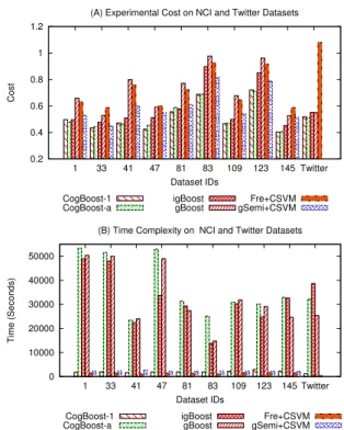
In this subsection, we evaluate the effectiveness of Cog-Boost for cost-sensitive learning and fast cutting-plane training in terms of average cost and runtime performance. The experimental results for NCI and Twitter graphs under default parameter settings are illustrated in Fig. 4.
Average Cost For average cost, Fig. 4. (A) demonstrates
that gBoost has the worst performance on 5 out of 10 datasets (i.e. the largest average cost). This is mainly because gBoost is a cost-insensitive algorithm, which con-siders that all training graphs are equally important in terms of their costs. As a result, gBoost fails to leverage the costs of graph samples to discover subgraph features mostly discriminative for differentiating graphs in the positive class, leading to deteriorated classification performance.
For igBoost, Fre+CSVM, and gSemi+CSVM, all of them have a mechanism to assign weight values to dif-ferent classes. Fig. 4. (A) shows that igBoost outperforms Fre+CSVM and gSemi+CSVM, which is mainly attributed to igBoost’s integration of discriminative subgraph selec-tion and classifier learning for graph classificaselec-tion. For Fre+CSVM and gSemi+CSVM, they decompose subgraph selection and classifier learning into two separated steps, without integrating them to gain mutual benefits, i.e., the subgraphs selected by frequency and gSemi score [7] may not be a good feature set for SVM learning. As a result, Fre+CSVM and gSemi+CSVM are inferior to igBoost.
This is, in fact, consistent with previous studies [5], which confirmed that gBoost outperforms a frequent subgraph based algorithm (mine frequent subgraphs as features and then apply SVMs).
The experimental results in Fig. 4 (A) show that Cog-Boost outperforms igCog-Boost. This is because the loss func-tion in igBoost is not a cost-sensitive loss funcfunc-tion, but heuristically adapted from the hinge loss function (i.e., simply assigning different weights to different classes). Therefore, it does not necessarily implement the Bayes decision rule and cannot guarantee minimum conditional risk.
In contrast, CogBoost-1 and CogBoost-a adopt an op-timal cost-sensitive loss function which implements the Bayes decision rule to achieve minimum cost. Evidently, both CogBoost-1 and CogBoost-a outperform gBoost over all graph datasets with significant performance gain, and outperforms igBoost for most graph datasets.
Runtime Performance The algorithm runtime in Fig.
4 (B) shows that gBoost, igBoost, and CogBoost-a all require an order of magnitude more time over CogBoost-1, Fre+CSVM, and gSemi+CSVM. For instance, CogBoost-1 only needs about 1,846 seconds on NCI-1 dataset whereas all other boosting algorithms take about over 50,000 sec-onds to complete the task. Overall, CogBoost-1 is 25 times faster the all other boosting algorithms. This result validates that reformulating our problem from Eq.(7) to a new problem (Eq. (10)) and using cutting plane algorithm to solve it can efficiently speed up the problem solving.
Note that Fre+CSVM and gSemi+CSVM have a little less runtime than CogBoost-1, this is because they only solve the SVM formulation (quadratic program) once, while our algorithm iteratively solves a linear program in each iterations.
Comparing the runtime of NCI and Twitter datasets, we found that although twitter dataset is significant larger than NCI, the time consumption for NCI and Twitter does not differ much. This is because the average number of nodes and edges for twitter dataset is much smaller than NCI, making it much efficient for subgraph mining for all algorithms.
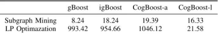
Runtime Consumption Details for Boosting algorithms
To better understand why CogBoost is more efficient than its peers, we investigate detailed runtime consumption in each step for boosting algorithms. These boosting methods all consist of two key steps in each iteration: i.e., optimal subgraph mining and linear problem solving. Accordingly, we report the algorithm runtime in each iteration in Fig. 6, and report average time consumption in Table 3.
Table 3 and Fig. 6 show that, on average, subgraph min-ing can be done in less than 20 seconds for all algorithms. At the first iteration, the subgraph mining step requires a significant amount of runtime. This is because gSpan needs to generate the search tree until the pruning condition is satisfied. Creating a new node is time consuming, because the list of embeddings is updated, and the minimality of the DFS code has to be checked (See [5] for more details). In the latter iterations, the time consumption for this process
0 200 400 600 800 1000 1200 1400 5 10 15 20 25 30 35 40 45 50 Time (seconds) No. of Iterations (A) Time consumption in each iteration for gBoost
Subgraph Mining Step LP Optimazation Step 0 200 400 600 800 1000 1200 1400 5 10 15 20 25 30 35 40 45 50 Time (seconds) No. of Iterations (B) Time consumption in each iteration for igBoost
Subgraph Mining Step LP Optimazation Step 0 200 400 600 800 1000 1200 1400 5 10 15 20 25 30 35 40 45 50 Time (seconds) No. of Iterations (C) Time consumption in each iteration for CogBoost-a
Subgraph Mining Step LP Optimazation Step 0 50 100 150 200 250 5 10 15 20 25 30 35 40 45 50 Time (seconds) No. of Iterations (D) Time consumption in each iteration for CogBoost-1
Subgraph Mining Step LP Optimazation Step
Fig. 6: Runtime performance in each iterations. Runtime consumption for (A) gBoost, (B) igBoost, (C) CogBoost-a, and (D) CogBoost-1.
TABLE 3:Average Time Consumption in Each Iteration (Seconds)
gBoost igBoost CogBoost-a CogBoost-l Subgraph Mining 8.24 18.24 19.39 16.33 LP Optimazation 993.42 954.66 1046.12 21.58
can be reduce greatly because the searching space can be reused. The node creation is necessary only if it were not created in previous iterations. As a result, we can observe that the algorithm is more efficient in the latter iterations.
As for the LP optimization steps, gBoost, igBoost, and a all consume much more time than CogBoost-1. This is because they all need to solve a linear problem (similar to Eq. (7) for gBoost and igBoost) with l slack variablesξi|i=1,···,l in each iteration (l is the total number
of graph examples). When l is large, it will require a very large amount of time to solve the linear problem. In contrast, CogBoost-1 solves the linear problem (Eq. (10)) with only one single slack variableξby using cutting plane algorithms (Algorithm 3). This new formulation can greatly reduce the time required for linear problem solving.
The results in Table 3 and Fig. 6 show that CogBoost-1 only needs about 21.58 seconds for one iteration while all other algorithms require about 1,000 seconds to complete this step. Because LP optimization step is the most compu-tationally intensive step for boosting algorithms, CogBoost-1 is much faster than all existing boosting algorithms for graph classification.
Comparison of CogBoost-1 and CogBoost-aThe
exper-iment results in Fig. 4 show that CogBoost-1 can always achieve similar (or very close) classification performance as CogBoost-a. This is because CogBoost-1 can always return an -tolerance solution to CogBoost-a in each it-eration. This, in fact, empirically proves the correctness of our CogBoost-1 formulation. Because CogBoost-1 can achieve accurate solutions to CogBoost-a but with much less runtime consumption than CogBoost-a, in the follow-ing experiments, we will report CogBoost-1 (termed as
CogBoost) for comparison with other algorithms.
0.2 0.4 0.6 0.8 1 1.2 5 10 15 20 25 Average Cost Value of C1 (A) Average Cost for NCI-1 gBoost igBoost CogBoost Fre+CSVM gSemi+CSVM 0.2 0.4 0.6 0.8 1 1.2 5 10 15 20 25 Average Cost Value of C1 (B) Average Cost for NCI-33 gBoost igBoost CogBoost Fre+CSVM gSemi+CSVM 0.2 0.4 0.6 0.8 1 1.2 5 10 15 20 25 Average Cost Value of C1 (C) Average Cost for NCI-41 gBoost igBoost CogBoost Fre+CSVM gSemi+CSVM 0.2 0.4 0.6 0.8 1 1.2 5 10 15 20 25 Average Cost Value of C1 (D) Average Cost for NCI-47 gBoost igBoost CogBoost Fre+CSVM gSemi+CSVM 0.2 0.4 0.6 0.8 1 1.2 5 10 15 20 25 Average Cost Value of C1 (E) Average Cost for NCI-81 gBoost igBoost CogBoost Fre+CSVM gSemi+CSVM 0.2 0.4 0.6 0.8 1 1.2 5 10 15 20 25 Average Cost Value of C1 (F) Average Cost for NCI-83 gBoost igBoost CogBoost Fre+CSVM gSemi+CSVM 0.2 0.4 0.6 0.8 1 1.2 5 10 15 20 25 Average Cost Value of C1 (G) Average Cost for NCI-109 gBoost igBoost CogBoost Fre+CSVM gSemi+CSVM 0.2 0.4 0.6 0.8 1 1.2 5 10 15 20 25 Average Cost Value of C1 (H) Average Cost for NCI-123 gBoost igBoost CogBoost Fre+CSVM gSemi+CSVM 0.3 0.6 0.9 1.2 1.5 1.8 1 2 3 4 5 Average Cost Value of C1 Average Cost for Twitter gBoost
igBoost Fre+CSVMCogBoost
Fig. 5: Average Cost with respect to differentC1 value
performance for cost-sensitive learning because the time complexity is relatively stable for each graph dataset with the same number of training graphs.
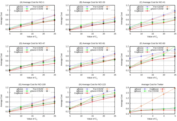
7.2.1 Performance w.r.t. different cost values
In order to study the algorithm performancew.r.t. different cost values, we vary the C1 values from 5 to 25 for NCI graphs and 1 to 5 for Twitter graphs and report the algorithm performance in Fig. 5 where the x-axis in each subfigure shows the C1 values and the y-axis show the average costs of different methods.
Fig. 5 shows that with the increasing of C1 value, the average costs of all all algorithms will increase. This is because the increasing ofC1 value results in a higher mis-classification cost of positive graphs. Comparing to gBoost, igBoost achieves less average cost on most graph datasets. This is mainly attributed to the uneven weight assignment scheme for different classes adopted in igBoost, which allows igBoost to deal with the cost-sensitive problem to some extend.
For all datasets, CogBoost achieves minimum average cost with respect to different C1 values. This is attributed to the optimal hinge loss function employed in CogBoost, which implements the Bayes decision rules and forces CogBoost to favor high cost samples in order to minimize the misclassification costs. This result is actually consistent with results from a previous study [22], which addresses cost-sensitive support vector machine algorithm for vector data, while CogBoost is a boosting algorithm for graph classification. 0.3 0.4 0.5 0.6 0.7 0.1 0.01 0.001 0.0001 0.00001 500 1000 1500 2000 2500
Average Cost Time (seconds)
Value of ε
(A) Time and Average Cost with Different ε on NCI-1 Time Cost 0.3 0.4 0.5 0.6 0.7 0.1 0.01 0.001 0.0001 0.00001 500 1000 1500 2000 2500
Average Cost Time (seconds)
Value of ε
(B) Time and Average Cost with Different ε on NCI-33 Time Cost
Fig. 7:Average cost (lefty-axis) and algorithm runtime (righty-axis) with respect to differentvalues (x−axis). (A) NCI-1, and (B) NCI-33
7.2.2 Performance w.r.t. differentvalues
In CogBoost, the parametercontrols CogBoost’s solutions in solving the cutting plane algorithm (Algorithm 3). In order to validate’s impact on the algorithm performance, we vary values and report CogBoost’s performance in Fig. 7.
Fig. 7 shows that for large values (e.g. = 0.1 on NCI-1 dataset), the corresponding average cost is also large. This is because a large value returns a solution far away from the optimal solution and results in poor performance for CogBoost. As continuously decreases (from 0.1 to 0.00001), the average cost on both NCI-1 and NCI-33 datasets decrease. This is because with a small value, CogBoost can return accurate solution for classification. However, the runtime consumption for smaller values will also increase because more iterations are required in the cutting algorithm. Our empirical results suggest that a moderate value (such as =0.01) has a good tradeoff between time complexity and average cost. So we set =0.01 as a default value in our experiments.
In summary, our experiments suggest that cost-sensitive graph classification is a much more complicated problem than traditional cost-sensitive learning, mainly because that graph classification heavily replies on subgraph feature exploration. Simply converting a graph dataset into a vec-tor representation, by using frequent subgraph features, and then applying cost-sensitive learning (like Fre+CSVM does) is far from optimal. Indeed, subgraph features play vital role for graph classification. By using a cost-sensitive subgraph exploration process and a cost-sensitive loss func-tion, CogBoost demonstrates its superb performance for cost-sensitive graph classification.
8
CONCLUSION
In this paper, we formulated a cost-sensitive graph classi-fication problem for large scale graph datasets. We argued that many real-world applications involve data with depen-dency structures and the cost of misclassifying samples in different classes is inherently different. This problem moti-vates us to consider effective graph classification algorithms with cost-sensitive capability and being suitable for large scale graph datasets. To solve the problem, we proposed a fast boosting algorithm, CogBoost, which embeds the costs into the subgraph exploration and the learning process. The boosting procedure utilizes an optimal loss function to minimize the misclassification costs by implementing the Bayes decision rule. To enable fast training on large scale graphs, a cutting plane formulation is derived so that the linear problem can be solved efficiently in each itera-tion. Experimental results on large real-life graph datasets validate our designs.
ACKNOWLEDGMENT
We thank the constructive comments from anonymous re-viewers. This work is partially supported by Australia ARC Discovery Project (DP140102206), and National ship for Building High Level Universities, China Scholar-ship Council (No. 2011630030).
R
EFERENCES[1] H. Kashima, K. Tsuda, and A. Inokuchi, Kernels for Graphs. Cambridge (Massachusetts): MIT Press, 2004, ch. In: Schlkopf B, Tsuda K, Vert JP, editors. Kernel methods in computational biology. [2] M. Fang and D. Tao, “Networked bandits with disjoint linear payoffs,” inProc. 20th ACM SIGKDD. ACM, 2014, pp. 1106– 1115.
[3] S. Pan, X. Zhu, C. Zhang, and P. S. Yu, “Graph stream classification using labeled and unlabeled graphs,” inProc. of ICDE. IEEE, 2013. [4] K. Riesen and H. Bunke, “Graph classification by means of lipschitz embedding,”IEEE Trans. on SMC - B, vol. 39, pp. 1472–1483, 2009. [5] H. Saigo, S. Nowozin, T. Kadowaki, T. Kudo, and K. Tsuda, “gboost: a mathematical programming approach to graph classification and regression,”Machine Learning, vol. 75, pp. 69–89, 2009. [6] Y. Zhu, J. Yu, H. Cheng, and L. Qin, “Graph classification: a
diversified discriminative feature selection approach,” in Proc. of CIKM. ACM, 2012, pp. 205–214.
[7] X. Kong and P. Yu, “Semi-supervised feature selection for graph classification,” inProc. of ACM SIGKDD, 2010.
[8] J. Tang and H. Liu, “An unsupervised feature selection framework for social media data,”IEEE Transactions on Knowledge and Data Engineering, vol. 26, no. 12, pp. 2914–2927, 2014.
[9] H. Fei and J. Huan, “Boosting with structure information in the functional space: an application to graph classification,” inProc. of ACM SIGKDD, 2010.
[10] J. Wu, X. Zhu, C. Zhang, and P. Yu, “Bag constrained structure pattern mining for multi-graph classification,”Knowledge and Data Engineering, IEEE Transactions on, vol. PP, no. 99, pp. 1–1, 2014. [11] S. Pan and X. Zhu, “Graph classification with imbalanced class
distributions and noise,” inIJCAI, 2013.
[12] P. Tiwari, J. Kurhanewicz, and A. Madabhushi, “Multi-kernel graph embedding for detection, gleason grading of prostate cancer via mri/mrs,”Medical Image Analysis, vol. 17, no. 2, pp. 219–235, 2013. [13] M. Deshpande, M. Kuramochi, N. Wale, and G. Karypis, “Frequent substructure-based approaches for classifying chemical compounds,”
IEEE TKDE, vol. 17, pp. 1036–1050, 2005.
[14] P. Domingos, “Metacost: a general method for making classifiers cost-sensitive,” inProc. of ACM KDD, 1999, pp. 155–164. [15] K. Veropoulos, C. Campbell, and N. Cristianini, “Controlling the
sensitivity of support vector machines,” inProc. of IJCAI, vol. 1999, 1999, pp. 55–60.
[16] C. Elkan, “The foundations of cost-sensitive learning,” in Inter-national joint conference on artificial intelligence, vol. 17, no. 1. Citeseer, 2001, pp. 973–978.
[17] S. Zhang, Z. Qin, C. X. Ling, and S. Sheng, “Missing is useful”: missing values in cost-sensitive decision trees,”IEEE TKDE, vol. 17, no. 12, pp. 1689–1693, 2005.
[18] F. R. Bach, D. Heckerman, and E. Horvitz, “Considering cost asymmetry in learning classifiers,”The Journal of Machine Learning Research, vol. 7, pp. 1713–1741, 2006.
[19] B. Zadrozny, J. Langford, and N. Abe, “Cost-sensitive learning by cost-proportionate example weighting,” in Proc. of IEEE ICDM, 2003.
[20] H. Masnadi-Shirazi and N. Vasconcelos, “Cost-sensitive boosting,”
IEEE PAMI, vol. 33, no. 2, pp. 294–309, 2011.
[21] A. C. Lozano and N. Abe, “Multi-class cost-sensitive boosting with p-norm loss functions,” inProc. of ACM KDD, 2008, pp. 506–514. [22] H. Masnadi-Shirazi and N. Vasconcelos, “Risk minimization,
prob-ability elicitation, and cost-sensitive svms,” inICML, 2010. [23] N. Abe, B. Zadrozny, and J. Langford, “An iterative method for
multi-class cost-sensitive learning,” inProc. ACM KDD, 2004, pp. 3–11.
[24] X. Zhu and X. Wu, “Class noise handling for effective cost-sensitive learning by cost-guided iterative classification filtering,”
IEEE TKDE, vol. 18, no. 10, pp. 1435–1440, 2006.
[25] S. Lomax and S. Vadera, “A survey of cost-sensitive decision tree induction algorithms,”ACM Computing Surveys, vol. 45, no. 2, 2013. [26] G. K. J. Shawe-Taylor, “Optimizing classifiers for imbalanced
train-ing sets,” inNIPS, vol. 11. MIT Press, 1999, p. 253.
[27] X. Yan and J. Han, “gspan: Graph-based substructure pattern min-ing,” inProc. of ICDM, Maebashi City, Japan, 2002.
[28] X. Wu, X. Zhu, G. Wu, and W. Ding, “Data mining with big data,”
IEEE TKDE, vol. 26, no. 1, pp. 97–107, 2014.
[29] S. Ranu and A. Singh, “Graphsig: A scalable approach to mining significant subgraphs in large graph databases,” inProc. of ICDE. IEEE, 2009, pp. 844–855.
[30] J. Wu, Z. Hong, S. Pan, X. Zhu, C. Zhang, and Z. Cai, “Multi-graph learning with positive and unlabeled bags,” inSIAM International Conference on Data Mining. SIAM, 2014, pp. 1–12.
[31] H. Fei and J. Huan, “Structure feature selection for graph classifi-cation,” inProc. of ACM CIKM, California, USA, 2008.
[32] N. Jin, C. Young, and W. Wang, “Graph classification based on pattern co-occurrence,” inProc. of ACM CIKM, 2009.
[33] M. Thoma, H. Cheng, A. Gretton, J. Han, H. Kriegel, A. Smola, L. Song, P. Yu, X. Yan, and K. Borgwardt, “Near-optimal supervised feature selection among frequent subgraphs,” inProc. of SDM, 2009. [34] T. Kudo, E. Maeda, and Y. Matsumoto, “An application of boosting to graph classification,” inProc. of NIPS, Vancouver, Canada, 2004. [35] J. Wu, S. Pan, X. Zhu, and Z. Cai, “Boosting for multi-graph
classification,”IEEE transactions on cybernetics, 2014.
[36] S. Pan, J. Wu, X. Zhu, and C. Zhang, “Graph ensemble boosting for imbalanced noisy graph stream classification.”IEEE transactions on cybernetics, 2014.
[37] W. Fan, S. J. Stolfo, J. Zhang, and P. K. Chan, “Adacost: misclassi-fication cost-sensitive boosting,” inICML, 1999, pp. 97–105. [38] H. Masnadi-Shirazi, N. Vasconcelos, and A. Iranmehr,
![Fig. 1: Training time w.r.t. different number of graphs on NCI-1 dataset for gBoost [5] and igBoost algorithm [11]](https://thumb-us.123doks.com/thumbv2/123dok_us/9788075.2470573/3.850.126.335.84.211/training-different-number-graphs-dataset-gboost-igboost-algorithm.webp)