Exposure at default models with and without the credit conversion factor

(1)

Contents lists available at ScienceDirect

European

Journal

of

Operational

Research

journal homepage: www.elsevier.com/locate/ejor

Decision

Support

Exposure

at

default

models

with

and

without

the

credit

conversion

factor

✩

Edward N. C. Tong

a,∗

_{, Christophe Mues}

b

_{, Iain Brown}

c

_{, Lyn C. Thomas}

b a_Bank_of_America,_One_Bryant_Park,_New_York,_NY_10036,_USA

b_Southampton_Business_School,_University_of_Southampton,_Southampton_SO17_1BJ,_United_Kingdom c_SAS_UK,_Wittington_House,_Henley_Road,_Marlow_SL7_2EB,_United_Kingdom

a

r

t

i

c

l

e

i

n

f

o

Articlehistory:

Received16February2014 Accepted25January2016 Availableonline1February2016

Keywords: Exposureatdefault Creditcards

Generalizedadditivemodels Regression

Riskanalysis

a

b

s

t

r

a

c

t

The Basel II and III Accords allow banks to calculate regulatory capital using their own internally developed models under the advanced internal ratings-based approach (AIRB). The Exposure at Default (EAD) is a core parameter modelled for revolving credit facilities with variable exposure. The credit conversion factor (CCF), the proportion of the current undrawn amount that will be drawn down at time of default, is used to calculate the EAD and poses modelling challenges with its bimodal distribution bounded between zero and one. There has been debate on the suitability of the CCF for EAD modelling. We explore alternative EAD models which ignore the CCF formulation and target the EAD distribution directly. We propose a mixture model with the zero-adjusted gamma distribution and compare its performance to three variants of CCF models and a utilization change model which are used in industry and academia. Additionally, we assess credit usage – the percentage of the committed amount that has been currently drawn – as a segmentation criterion to combine direct EAD and CCF models. The models are applied to a dataset from a credit card portfolio of a UK bank. The performance of these models is compared using cross-validation on a series of measures. We ﬁnd the zero-adjusted gamma model to be more accurate in calibration than the benchmark models and that segmented approaches offer further performance improvements. These results indicate direct EAD models without the CCF formulation can be an alternative to CCF based models or that both can be combined.

1. Introduction

The BaselII and III Accords deﬁne the standardsfor calculat-ing regulatory capital requirements for banks across the world (Basel Committee on Banking Supervision, 2005, 2011). Under the Advanced Internal Ratings-Based approach (AIRB), banks are allowedtoassesscreditrisk usingtheir owninternallydeveloped modelswhichtargetthreekeyparameters foreach creditfacility: (i)ProbabilityofDefault,PD,(ii)Loss GivenDefault,LGDand(iii) ExposureatDefault,EAD.Theseparameter estimatescanbeused toproduce an estimate forthe expectedloss (EL) orto estimate theunexpectedlossforwhichbanksmustholdcapital.Beyondthe purpose of calculating regulatory capital, these three parameters havewiderangingusesforbanks,servingasinputsintoeconomic

✩ _The_views_expressed_in_the_paper_are_those_of_the_authors_and_do_not_represent

theviewsoftheBankofAmerica. ∗ _{Corresponding}_author.

E-mailaddresses:[email protected](E.N.C.Tong),[email protected]

(C.Mues),[email protected](I.Brown),[email protected](L.C.Thomas).

capital models, stress testing, impairment forecasting, pricing and informingportfolio management across retail, corporate and wholesaleportfolios.

Inretail creditrisk, PD modelling hasbeenthe main focusof creditresearchforseveraldecadesandinrecentyears,LGDmodels withchallengingbimodaldistributionshavealsobeenthefocusof research (Loterman, Brown,Martens, Mues, & Baesens,2012). Al-though EAD distributions are comparatively asdiﬃcult tomodel, theyhavereceivedmuchlessattentionintheliterature.

For credit card and overdraft portfolios, EAD estimation has proven a hard problem to tacklein practice. Forﬁxed exposures suchasresidential mortgagesandpersonal loans,theestimatefor EADcansimplybetakenfromthecurrenton-balanceamountand littleifanymodellingisrequired.Forcreditcardsthough,the re-volving natureofthecredit lineposeschallengeswithregardsto predictingtheexposure atdefaulttime. Ascredit cardcustomers may borrow moremoney in the months prior to default, simply takingthecurrentbalancefornon-defaultedcustomerswouldnot produceaconservativeenoughestimatefortheamountdrawnby thetime ofdefault. The EADcould partiallybe driven bycurrent http://dx.doi.org/10.1016/j.ejor.2016.01.054

(2)

or recent customer behaviour (i.e. credit usage, drawn, undrawn amounts,changestoundrawnamountsovertime).Asanexample of two distinct behaviour groups, some customers, classiﬁed as transactors,tendtopayoff theirentirebalanceattheendofeach monthwhileothers,termedrevolvers,tendtopayoff onlypartof themonthlybalanceandhenceincurinterestcharges(So,Thomas, Seow,&Mues,2014).

ToestimatetheEADforcreditcardsorotherformsofrevolving credit,theBaselII/IIIAccordhassuggestedtheuseofhistoricdata to evaluatetheCreditConversion Factor(CCF),i.e.the proportion ofthecurrentundrawnamountthatwilllikelybedrawndownat time ofdefault(Valvonis,2008).The Accorddidnotexplicitly re-quireEADmodelstouseCCFcalculations;however,CCFsare reg-ularlyreferred tointheAccord.Oncea CCFestimate isproduced fora(segmentof)variableexposure(s),theEADisthengivenby: EAD=CurrentDrawnAmount+(CCF×CurrentUndrawnAmount). With this (indirect) approach, the accuracy of EAD prediction is obviously linked to thequality of theCCF modelandsuch mod-ellinghasposedsubstantialchallengesbecausethedistributionof CCFdoesnotconformtostandardstatisticaldistributions.CCF dis-tributions tend to be highly bimodal with a probability mass at zero(no change inbalance), anotheratone (borrowinghas gone uptothecreditlimit),andarelativelyﬂatdistributioninbetween, notunlikesomeLGDdistributions(Lotermanetal.,2012). Further-more,in manyCCF datasets,one mightseea substantialnumber ofnegativeCCFsandCCFsgreaterthanone(anexampleofthe lat-termaybewherethecreditlimithasincreasedbetweenthepoint of observationandthe time of default, allowing the customer to go overtheoriginal limit);sincetheﬁnal modelestimates them-selves wouldhavetobe constrainedbetweenzeroandone, such individualobservationsaresometimestruncatedtozeroorone, re-spectively(Jacobs,2010).

Traditional regression modelling with ordinary least squares (OLS) may be less suitable forthe CCF because predictedvalues maybe lessthan zeroorgreater thanone,leadingtoinvalid CCF predictions.Additionally,thenon-normalityoftheerrorterm un-derminesmanyoftheOLStests.Standardlogisticregression com-monly used forPD models would also be inappropriate because theCCFresponsevariableisproportionalandnotbinary. Appropri-atediscretization oftheCCF response wouldbe necessary,which could result in some information loss, or alternatively, fractional responseregressionshouldbeconsidered.

Taplin,Minh To, andHee, 2007haveargued that theCCF for-mulation is problematic because the bounded CCF distribution forces EADto be equal tothe credit limitwhen CCF equals 1.In practice,itiscommontoﬁndaccountswithEADgreaterthanthe creditlimitfromchargesaccruedduetoadditionalpurchasesover thelimitandinterestcharges,orcreditlimitchanges.Theauthors insteadsuggestedmodelsthatpredictEADdirectlyandignorethe CCF formulation.However, Yang andTkachenko (2012) have con-tended thatCCF modelsare moresuitablegiventhat theEAD re-sponsevariablemaybetoostatisticallydiﬃculttomodelgiventhe granular scale of currency amounts and that the CCF formula is less prone to such scaling issues with its range being limitedto theunitinterval.

Theaimsofthispaperaretoempiricallyassessalternative sta-tisticalmethods formodellingthe EADby targetingthe EAD dis-tributiondirectlyratherthanfocusingontheCCF;toevaluatethis, we usea creditcardportfoliofroma largeUK bank.We hypoth-esize that competitive EAD modelscan be developedby ignoring the CCF formulation and instead selecting EAD as the response variable in a statistical model. Two different direct EAD models areconsidered– anOLSmodelandazero-adjustedgammamodel (Rigby,&Stasinopoulos,2005,2007).

The zero-adjustedgamma (ZAGA)model wasexplored to deal withthepositivelyskewednatureofEADandconsideringitsprior

use in predicting the LGD amount of residential mortgage loans (Tong, Mues, & Thomas, 2013). In this model, the EAD amount is modelled as a continuous response variable using a semi-parametricdiscrete-continuous mixturemodel approachwith the zero-adjustedgammadistribution.Firstly,asthenon-zeroor pos-itiveEADamountdisplaysright-skewness,itismodelledwiththe gammadistribution.ThemeananddispersionofthepositiveEAD amountare modelledexplicitlyasafunction ofexplanatory vari-ables.Secondly, theprobability of the(non-)occurrence ofa zero EAD amountis modelledwitha logistic-additive model.All mix-turecomponents,i.e.thelogistic-additivecomponentforthe prob-abilityofzeroEADandthelog-additivecomponentsforthemean anddispersion of the EAD amount conditional on there beinga non-zero EAD, can be estimated using account-level behavioural characteristics.

TheperformanceofthesedirectEADmodelsarebenchmarked againstthreeCCFmodels(withCCFastheresponsevariable)using OLS, Tobit and fractional response regression and the utilization change model. These approaches are established methods used inindustry and/or academia forEAD andLGDmodelling(Brown, 2011;Bellotti&Crook,2012;Bijak&Thomas,2015).

When borrowers are already close to maxing out the credit lineandtheundrawnamountislow,theCCF can becomehighly volatileandmodelperformance maybe compromised(Qi,2009). Therefore, a combined approach is suggested that segments on credit usage (i.e. utilization rate, or the percentage of the com-mittedamountthathasbeencurrentlydrawn)andthenusestwo separatemodels,witheithertheCCForEADastheresponse vari-able,dependingontheutilizationsegmentthatthecreditcardfalls into.Wehypothesizethat thecombineduseofCCFmodellingfor accountswithlow utilizationanddirectEADmodelsforaccounts withhighutilizationmayimprovetheoverallmodelperformance. Ourdatasetincludedtime todefaultasavariable.Inpractical modeldevelopment, thisvariable would be considered unknown a priori for each customer and would not typically be used as a candidate covariate in predictive model ﬁtting. Nonetheless, it hasbeenused inprevious empiricalstudies tostudyexplanatory driversofCCF(Moral,2011;Brown,2014;Jacobs,2010).Therefore, discardingitwouldmakeourresultslesscomparabletothose re-portedby others.Furthermore,itwouldbe interesting toexplore this time effect on the various components of the ZAGA model, particularlythedispersioncomponentasonewouldintuitively ex-pecttheerrorvariancetoincreasethemoretimeelapsesbetween thepointofobservationanddefault.

Toallow a model with time to defaultas one of its explana-toryvariables to be applied to a prediction task, we propose an additionalsurvivalanalysismodelcomponent.Survivalanalysishas previously beenemployed tomodeltime to defaultinretailloan portfolios, providing insight into factors that predict when con-sumersaremorelikelytodefault(Stepanova&Thomas,2002; Ma-lik&Thomas,2010;Tong,Mues,&Thomas,2012).Similarly,we de-velopaPDmodelusingtheCoxproportionalhazardsmodel(Cox, 1972;Hosmer, Lemeshow, & May, 2008) with time to defaultas theeventof interestbutwiththe length ofthecohort periodas time horizon. Wethen show how theresulting monthlyPD esti-matescan becombinedwithan EAD modelthathastime to de-faultincludedasacovariate.ThismethodformodellingEADusing a consistent probabilistic deﬁnition and a direct EAD estimation approachwasproposed byWitzany (2011).Theirresearch termed thismethodthe‘weightedPDapproach’andsuggestedtheuseof defaultintensitiestoestimate EADbyconsideringthetimeto de-fault.Ourpaperextendstheirworkbyusingarealbankingdataset andexplicituseoftheCoxproportionalhazardsmodel.Leowand Crook (2015) have also combined survival and panel modelling methodscomprisingcreditlimitanddrawnbalancemodelsto pre-dict EAD for credit cards. We suggest thismethod could further

(3)

incorporatethetimetodefaultasapredictivecovariateinanEAD modeltoimprovemodelperformance.

The novel aspects of our studythus are that we (1)evaluate whethercompetitive EAD models can be developed by targeting the EAD distribution directly without using a CCF component, (2) assess credit usage as a segmentation criterion allowing us to combinetwo types of EAD models to further improve perfor-mance,(3)comparethe performanceof thesenewapproachesto CCF and utilization change models commonly used in industry and/or academia and (4) propose an additional survival analysis component to allow the use of time to default as a predictive covariate in EAD modelling. All models will be assessed out-of-sample using cross validation on a series of discrimination and calibrationmeasures.

The remainderofthe paperisorganizedasfollows.InSection 2, an overviewofthedataset along withtheapplicationand be-havioural characteristics used for the EAD models will be pre-sented.Thestatistical andvalidationmethods usedin our exper-imentsare discussedinSection3.Next,theresultsofthemodels arediscussedinSection 4.Section 5willconcludethepaperand suggestsomefurtheravenuesforresearch.

2. Data

Thedatasetconsistedof10,271observationsofaccountsfroma majorUK bank. Thedataset derived fromacredit cards portfolio observedover a three yearperiod fromJanuary 2001 to Decem-ber2004. Intheabsence ofadditionaldataaboutother potential defaulttriggers, forthe purposeof thisstudy, a defaultoccurred whenacharge off orclosurewasincurred onthecredit card ac-count.Achargeoff inthiscasewasdeﬁnedasthedeclarationby thecreditorthatanamountofdebtisunlikelytobecollected, de-claredatthepointof180daysor6monthswithoutpayment.To computetheobservedCCFvalue,theoriginaldatasetwasdivided intotwo twelve-monthcohorts.Theﬁrstcohortranfrom Novem-ber2002toOctober2003andthesecond cohortfromNovember 2003toOctober2004.InthecohortapproachforCCF,discrete cal-endarperiodsareusedtogroupdefaultedfacilitiesinto12-month periods,accordingtothedateofdefault. Data wasthen collected oncandidateEADrisk factorsanddrawn/undrawnamountsatthe beginningofthecalendarperiodanddrawnamountatthedefault date.

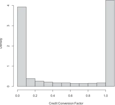
Fig.1showstheempiricalCCFdistributionaftertruncation;the meanCCF value herewas0.515 (sd=0.464).The value issimilar to that of S&P and Moody’sdefaulted borrowers’ revolving lines ofcreditfrom 1985to 2007,asreportedby Jacobs (2010); there, thetruncatedmeanwas0.422(sd=0.409).Notethat thebimodal nature of Fig. 1 shows similarities to reported LGD distributions (Lotermanetal.,2012;Bellotti& Crook,2012). Fig.2displaysthe distribution we observed for the EAD, clearly showing the posi-tivelyskewednatureofthisvariable.Pleasenotethatsomeofthe scalesontheﬁguresinthisstudyhavebeenremovedfordata con-ﬁdentialityreasons.

AsshowninTable1,atotalof11candidatevariableswere con-sideredforthemodels.TheﬁrstsixcandidatevariablesinTable1 were suggested by Moral (2011). They were generated from the monthlydataineachofthe cohorts,wheretd is thedefaultdate andtristhereferencedate(i.e.thestartofthecohort).Thelatter ﬁvevariableswerepreviouslysuggestedinBrown(2011),withthe aimofimprovingthepredictiveperformanceofthemodels.

The creditconversionfactorforaccounti,CCFi,wascalculated astheratiooftheobservedEADminus thedrawnamountatthe startofthecohortover thecreditlimit atthestartofthe cohort minusthedrawnamountatthestartofthecohort,i.e.:

CCFi=

E

(

td

)

i−E

(

tr

)

i L

(

tr

)

i−E

(

tr

)

i

(1)

Fig.1. Distributionofthecreditconversionfactor(aftertruncation).

Fig.2. Distributionofobservedexposureatdefault.

3. Statisticalmodels

Thefollowingsectionsoutlinethedifferentstatisticalmodelling approaches used to regress the EAD, CCF or utilization change againstthecandidatedriverslistedinTable1.ThedirectEAD mod-els(i.e.thosewithEADastheresponsevariable) aredescribedin Section 3.1. The three types ofCCF models used are outlined in Section 3.2. The utilizationchange model isdescribed in Section 3.3.Thesegmentedmodelsare introduced inSection3.4andthe survival modeladd-onis outlinedinSection 3.5.Finally,the pro-cessofmodelvalidationandtestingisdescribedinSection3.6. 3.1. DirectEADmodels

3.1.1. Zero-adjustedgammamodel

Thecreditcardsportfolioisstratiﬁedintotwogroups,theﬁrst group having zero EAD (in the absence of furtherdata, we have

(4)

Table1

CandidatevariablesconsideredforEADmodels.

Variable(s) Notation Description

Committedamount L(tr) Advisedcreditlimitatstartofcohort

Drawnamount E(tr) Exposureatstartofcohort

Undrawnamount L(tr)−E(tr) Limitminusexposureatstartofcohort

Drawnpercentage E(tr)

L(tr) Exposureatstartofthecohortdividedbycreditlimitatstartofthecohort(also commonlyreferredtoasutilizationrateorcreditusage)

Timetodefault td−tr Defaultdateminusreferencedate(months)

Ratingclass R(tr) Behaviouralscoreatstartofcohortgroupedinto4bins:(1)AAA-A,(2)BBB-B,(3)C,

(4)Unrated

Averagedaysdelinquent Averagenumberofdaysdelinquentinprevious3,6,9,or12months Undrawnpercentage L(tr)−E(tr)

L(tr) Undrawnamountatstartofcohortdividedbycreditlimitatstartofcohort Limitincrease Binaryvariableindicatingincreaseincommittedamountsince12monthspriorto

startofcohort

Absolutechangedrawn Absolutechangeindrawnamount:variableamountattrminusvariableamount3,6

or12monthspriortotr

Relativechangedrawn Relativechangeindrawnamount:variableamountattrminusvariableamount3,6or

12monthspriortotr,dividedbyvariableamount3,6or12monthspriortotr,

respectively.

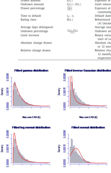
Fig.3. Candidatecontinuousdistributionsfornon-zeroEADontrainingset.

to assume these maypotentially include a number of special or technicaldefaultcases,charge-offsrelatedtootheraccounts, trun-cated/rounded observations, transfers of the outstanding amount to other repayment arrangements, orthey could be the resultof late paymentssubsequentto thedefaulttriggerentering theEAD calculation)andasecond grouphavingnon-zero EADs.Thelatter appears to have a continuouspositively skewed distribution (see Fig.3)andaccountsforthelargemajorityofcases.

Lety_idenotetheEADobservedfortheithaccount,i₌1,...,n(for simplicity, the indexi will be omitted from here on); x will be used todenotethe vectorof covariatesobserved fortheaccount. Amixeddiscrete-continuousprobabilityfunctionforycanthenbe speciﬁedas:

f

(

y

)

=

π

ify=0

(

1−

π

)

g

(

y

)

ify>0 (2)

whereg(y)isthedensityofacontinuousdistributionand

π

isthe probabilityofzeroEAD.

Fig.3 showsdifferentcandidatedistributions forg(y) ﬁttedto the non-zero EADs. Three positively skewed distributions were

explored:the gamma, inverse Gaussian and log normal distribu-tions;thenormaldistributionisshownasareferencecomparison. The candidate distributions were fitted onto a training set of a random representative sample. Fig. 3 indicates that the gamma distribution produced the most suitable fit for the histogram of positive EADs. There was further support for the fitted gamma distributionasitproduced thelowestAkaikeInformation Criteria (AIC) when compared to the inverse Gaussian and log normal distributions. The zero-adjusted gamma distribution was hence selectedto modelf(y). The resultingmodelwill be referredto in thispaperasZAGA-EAD.

The probability function of the ZAGA

(

μ

,

σ

,

π

)

model, a mixed discrete-continuous distribution, is deﬁned by Rigby and Stasinopoulos(2010): f

(

y

|

μ

,

σ

,

π

)

=

π

ify=0

(

1−

π

)

Gamma

(

μ

,

σ

)

ify>0 for0≤y<∞,

where0<

π

<1,mean

μ

>0,dispersion

σ

>0, Gamma

(

y,

μ

,

σ

)

= 1

(

σ2_μ

)

1/σ2 y 1 σ2−1 e−y/

(

σ2μ

)

₍

1/σ2

)

(3) with: E

(

y

)

=

(

1−

π

)

μ

andVar

(

y

)

=

(

1−

π

)

μ

2

_π

₊

_σ

2

₍₄₎

The ZAGA-EAD model is implemented using the Generalized Additive Models for Location, Scale and Shape (GAMLSS) frame-workdevelopedbyRigbyandStasinopoulos(2005).Theirapproach allows a range of skewed and kurtotic distributions to explic-itly model distributional parameters that may include the loca-tion/mean,scale/dispersion,skewnessandkurtosisasfunctionsof explanatoryvariables. GAMLSS also allows ﬁtting ofdistributions that do not belong to the exponential family as provided in the GeneralizedLinearModel(GLM)(Nelder&Wedderburn,1972)and GeneralizedAdditiveModel(GAM)frameworks(Hastie,Tibshirani, &Friedman,2009).

TheGAMLSSapproachisasemi-parametricmethodthatallows the relationship between the explanatory variables andresponse variabletobemodelledeitherparametrically(e.g.wherelinearity ismet),ornon-parametrically,usingsplinesmoothers,thelatterof whichisakeyfeatureoftheGAMapproach.

TherearethreecomponentstotheZAGA-EADmodel.Themean,

μ

,anddispersion,

σ

,ofanon-zeroEADandtheprobabilityofzero EAD,

π

, are modelled as a function of the explanatoryvariables

(5)

usingappropriaterespectivelinkfunctions: log

(

μ

)

=

η

1=x1

β

1+ J1 j=1 hj1

xj1

log

(

σ

)

=

η

2=x2

β

2+ J2 j=1 hj2

xj2

logit

(

π

)

=

η

3=x3

β

3+ J3 j=1 hj3

xj3

(5) wherexk

β

k denoteparametric terms,hjk(xjk) are non-parametric termssuch assmoothing splinesandwithk=1,2,3forthe dis-tributionparameters (hence, each modelcomponentcan haveits own selection of covariates). The dispersion of non-zero EAD is the squared coeﬃcient of variation,

δ

2_/

_μ

2_, _from _the _exponential

familyforthegammadensityfunction(McCullagh&Nelder,1989) where

δ

2 _denotes _the_variance _of _the _non-zero _EAD _{distribution.}

Thehjk(xjk)functionsaremodelledwithpenalizedB-splines(Eilers & Marx, 1996). Such non-parametric smoothing terms have the abilityto ﬁndnon-linearrelationships betweentheresponse and predictorvariables (Hastie etal., 2009). Penalized B-splines were chosenbecausetheyareabletoselectthedegreeofsmoothing au-tomaticallyusing penalizedmaximum likelihood estimation.This selection was done by minimizing the Akaike Information Crite-rion, i.e. AIC=−2L+kN, with L the log (penalized) likelihood, k thepenaltyparameter(setto2),andNthenumberofparameters intheﬁttedmodel(Akaike,1974).Automaticselectionof smooth-ingmaysuggestnon-linearorlinearrelationshipstotheresponse variableasdiscoveredinthedata.

Eachaccount,i,inthismodelisassociatedwithaprobabilityof zeroEAD,

π

i,andanon-zeroEADamount,yi.Thesepairsarethen usedtoformthefollowinglikelihoodfunction:

L= n i=1 f

(

yi

)

= yi=0

π

i yi>0

(

1−

π

i

)

Gamma

(

μ

i,

σ

i

)

(6) AnalgorithmdevelopedbyRigbyandStasinopoulos(2005)was used,whichisbased onpenalized(maximum)likelihood estima-tion.Theestimatesoftheprobability ofzeroEAD,meanand dis-persion of g(y) are used to compute an estimate for f(y) which combinestheprobability of EADandthe EAD amountgiventhat thereisanon-zeroEAD.

The modelwas developed andimplemented using the gamlss packagebyRigbyandStasinopoulos (2007)inR 3.0.1 software(R DevelopmentCoreTeam,Vienna,Austria).

3.1.2. Ordinaryleastsquares

The second direct EAD model was based on a standard OLS regression of the EAD response (untransformed) against the ex-planatory variables. We denote this model as OLS-EAD. A parsi-moniousmodelwasselectedthroughstepwiseselectionand back-wardeliminationbasedona5percent

α

-level.

3.2.CCFmodels

ThreemodelscomprisingOLS,Tobitandfractionalresponse re-gressionweredeveloped topredict theCCF (ratherthan theEAD directly).An account-level estimate forEAD isthen derived from thepredictedCCFasfollows:

EAD=CurrentDrawnAmount+

(

CCF×CurrentUndrawnAmount

)

(7)

Firstly,astandardOLSregressionmodel,denotedOLS-CCF,was ﬁttedfortheCCFtarget.Secondly,aTobitregressionmodel(Tobin, 1958; Greene, 1997), denoted Tobit-CCF, was developed, which treats observations with CCF below zero and above one as cen-sored withtheresponse only observedinthe interval [0,1]. The Tobitmodelassumesa latentvariabley∗,forwhichthe residuals conditionaloncovariatesxarenormallydistributed.Thetwo-sided Tobitmodelisgivenby:

y∗=x

β

+

ε

(8)

wherey∗

|

x∼N

(

μ

,

σ

2

₎

_and

y=0,ify∗≤0,

=y∗,if0<y∗<1,

=1,ify∗≥1 (9)

Maximum likelihood estimates are obtained for the

β

coeﬃ-cients;forfurtherdetailswerefertoGreene(1997).

Thirdly,afractionalresponseregression(denotedFRR-CCF)was run. This model has been used for modelling bimodal LGD dis-tributions ofcreditcards andcorporateloan portfolios(Bellotti& Crook, 2012; Qi & Zhao, 2011). FRR is a quasi-likelihood method proposed by Papke andWooldridge (1996)to model a fractional continuousresponsevariableboundedbetweenzeroandone,with validasymptoticinferenceandisgivenby:

E

CCF

|

x

=F

x

β

(10)

wherexisavectorofexplanatoryvariables,

β

isavectorof coeﬃ-cientsandF()representsthelogisticfunctionalformwhichensures thatpredictedvaluesareconstrainedbetweenzeroandone. F

x

β

= 1

1+exp

−x

β

(11)

To estimate the

β

coeﬃcients, the log-likelihood function is maximized,i.e.thesumoverallaccountsof:

l

β

=CCF×log

F

x

β

+

(

1−CCF

)

×log

1−F

x

β

(12) SimilarlytothedirectEADmodels,variableselectionforallCCF models wasperformed through stepwise selection and backward elimination. The OLS-EAD and all three CCF models were devel-opedwithSAS9.3software(SASInstituteInc.,Cary,NC,USA). 3.3. Utilizationchangemodel

An alternative benchmark model, which has been popular in industry, was developed based on the facility utilization change (Yang &Tkachenko,2012).Theutilizationchangemodelsthe out-standingdollar amount changeas a fractionofthe current com-mitmentamountandisdeﬁnedforaccountias

util=E

(

td

)

i−E

(

tr

)

i L

(

tr

)

i

(13) A Tobit model, denoted Tobit-UTIL, was ﬁtted as in Eq. (8) which treats observationswithutil belowzeroand above oneas censoredhencetheresponseisonlyobservedintheinterval[0,1]. 3.4. Creditusagesegmentationmodel

Segmentedmodelsweredevelopedusingthecreditusage vari-able topartition accountsinto low andhighutilization accounts. ACCFmodelwasthenﬁttedtothelow usagesubset ofthedata, anEAD modeltothelatter.Sensitivityanalysiswasusedto iden-tifyanoptimalcreditusagecut-off forthepartitioning.Model cal-ibration performance was evaluated by varying the credit usage segmentationcut-pointfrom10percentto95per cent.The cut-off thatproduced thehighestcalibrationperformance (i.e. lowest

(6)

MAE,RMSE;cf.Section3.6)wasselected.Whenacut-off was iden-tiﬁed,low usageaccountsweremodelledwithanFRR-CCFmodel since thisis themodelthat achieved thehighestcalibration per-formance among the CCF models considered earlier. High usage accounts were tackledwith OLS-EAD andZAGA-EAD models. We denote the two resulting segmentation models by OLS-USE (the onecomprisingFRR-CCFandOLS-EAD)andZAGA-USE(i.e.FRR-CCF combinedwithZAGA-EAD),respectively.

3.5. SurvivalEADmodel

To allow the time to default variable to be used as an ex-planatory variable in practical model development, we propose thataSurvivalPDmodelbedevelopedandappliedinconjunction withthe EADmodel,we termthiscombinationtheSurvival EAD model.Thetime todefaultvariableisunknown aprioriand can-notbeusedforpredictivemodellingwithconventionalEADmodel frameworks. To avoid having to discard the variable, a Survival PD model component was developed with the Cox proportional hazards(PH)approach.Severalaforementionedmodels,Tobit-CCF, FRR-CCF, Tobit-UTIL, ZAGA-EAD and ZAGA-USE, with time to de-faultasanexplanatoryvariable,wereconsideredfortheEAD com-ponent.

The semi-parametric approach in hazard formfor theCox PH modelisgivenby:

h

t

|

x

=h0

(

t

)

exp

x

β

(14)

where h

(

t

|

x

)

is the hazard ordefault intensity attime t condi-tional ona vector ofexplanatoryvariables x, andinwhich h0(t)

is the baseline hazard, i.e., the propensity of a default occurring aroundt(giventhatithasnotoccurredyet)whenallexplanatory variables are zero.The baseline hazard is left unspeciﬁedforthe CoxPHmodel.

CombiningestimatesfromtheCoxPHandEADmodels,we cal-culatetheexpectedEADforaccounti,asfollows:

EAD= 12 t=1 [S

(

t−1

)

−S

(

t

)

] 1−S

(

12

)

×EAD

(

t

)

(15) whereS

(

t

)

isthesurvivalfunctionattimet,[S

(

t₋1

)

₋S

(

t

)

]thus givestheprobabilityofdefaultoccurringinthetthmonth accord-ing to theCox PHmodel,andEAD

(

t

)

isthe EAD modelestimate (according to Tobit-CCF,FRR-CCF, Tobit-UTIL, ZAGA-EAD or ZAGA-USE)conditionalonthetimetodefaultbeingt.Hence(15)allows us to produce estimatesof EAD without any prior knowledge of thetimetodefaultvariable.

Note that,to produce validEAD estimates,the horizonlength for theCox model mustbe the length ofeach cohortperiod (12 months)andtheoriginoftimeistakentobethestartofthe co-hortperiodinwhichdefaultoccurs;thismeansnoeventtime cen-soring isobserved in the data and each of theproduced default probabilitiesareindeedconditionalontheaccountdefaultingover thecohortperiod(i.e.S(12)₌0).One couldarguethat,inthe ab-senceofcensoring, other(non-survival) regressionmethods could alsobeconsidered,butitsﬂexible baselinehazardstill makesthe Cox PHmodel an attractive candidate formodelling time to de-fault.TheCoxPHmodelwasdevelopedwithSAS9.4software(SAS Institute Inc., Cary, NC, USA). Table 8 displays the results of the modelsﬁttedusing(15).

3.6. Modelvalidationandtesting

To assess the out-of-sample performance of the models thoroughly, 10-fold cross validationwas conducted on the entire sample of accounts on a series of discrimination and calibration measures. All measures were derived from account-level EAD

predictions (either direct ones or produced indirectly through a predictedCCF)tohaveacommonbaseofcomparison.Toevaluate discriminatory power (i.e. the models’ ability to discriminate between different levels of EAD risk), the Pearson r and Spear-man’s

ρ

correlation were computed. The Pearson r measures linearassociationandtheSpearman’s

ρ

correlation measures the correlationbetweenthe rankorderings ofobservedandexpected EADs. Calibration performance (here seen as the model’s ability to come up with accurate account-level estimates of EAD) was assessedwith themeanabsoluteerror(MAE)andthe rootmean square error (RMSE). A normalized version of these measures was also produced, where MAE and RMSE were calculated for EAD/Commitment Amount, which facilitated a percentage inter-pretation. These measures were termed MAEnorm and RMSEnorm

respectively. 4. Results

Next,wepresentthe resultsobtainedfora directEAD model, two competing CCF models, the sensitivity analysis of the seg-mented model and the cross-validated performance measures to compareall models (reported valueshereare averages overeach 10runs).Finally,weshowtheﬁndingsfortheaddedsurvival com-ponent.

4.1. ZAGA-EADmodelparameters

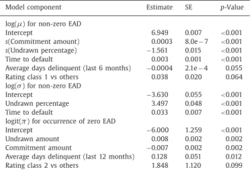
TheparametersofarepresentativeZAGA-EADmodelareshown inTable 2, withthe threesub-components for the occurrenceof zeroEAD,meanofnon-zeroEADanddispersionofnon-zeroEAD:

π

,

μ

and

σ

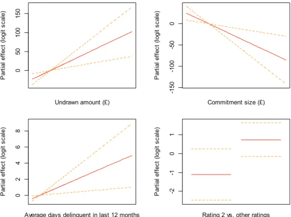
, respectively. The parameters ﬁttedwith splinesare denoted by s(.) in the table. The other estimates without spline functions are either ﬁtted as categorical variables or linearly as continuousvariables.

Fig.4 showsthe partial effectplots on logodds scalefor the occurrence ofzero EAD. Theseplots can be useful for interpret-ingcoeﬃcientestimates.Forexample,largerundrawnamountsare associatedwitha higherpropensity (andprobability)ofzeroEAD (seetop-leftplot)andlargerexposurecommitmentcorrespondsto a lower propensity of zeroEAD (see top-right plot). Precision of theestimatescanbegaugedwith95percentconﬁdenceintervals representedasdashedlines.

Forexample, in Fig.4, the partial effect of Rating 2 vsOther Ratings is shown as approximately −1 on the logit or log odds

Table2

Zero-adjustedgammamodel(ZAGA-EAD)basedonarepresentativetraining sam-ple.

Modelcomponent Estimate SE p-Value

log(μ)fornon-zeroEAD

Intercept 6.949 0.007 <0.001

s(Commitmentamount) 0.0003 8.0e−7 <0.001 s(Undrawnpercentage) −1.561 0.015 <0.001 Timetodefault 0.003 0.001 <0.001 Averagedaysdelinquent(last6months) −0.0004 2.1e−4 0.055 Ratingclass1vsothers 0.038 0.020 0.064 log(σ)fornon-zeroEAD

Intercept −3.630 0.055 <0.001

Undrawnpercentage 3.497 0.048 <0.001 Timetodefault 0.033 0.007 <0.001 logit(π)foroccurrenceofzeroEAD

Intercept −6.000 1.259 <0.001

Undrawnamount 0.008 0.002 0.002

Commitmentamount −0.007 0.002 0.002 Averagedaysdelinquent(last12months) 0.128 0.051 0.012 Ratingclass2vsothers 1.848 1.120 0.099

(7)

Fig.4. PropensityofzeroEADforzero-adjustedgammamodel.

scale, which represents the propensity of zero EAD after adjust-ment for the effect of other covariates in the model. Hence the oddsfortheoccurrenceofzeroEADwouldreduceby63percent

(

1−e−1

₎

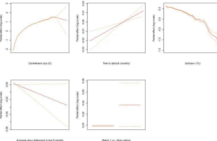
_for_Rating₂_vs_other_Ratings.

Importantly, Fig.5 showsthe partialeffects forthe meanand Fig.6 thedispersion ofnon-zero EAD. Forexample,the commit-ment size/amount plot in Fig. 5 suggests higher committed ex-posure islinked tolarger EAD, butthe relationship is non-linear (whichcould inpartbe explainedby theloglink functionused). AlongertimetodefaultisalsoassociatedwithhigherEAD.Allof theeffectsencounteredappeartobeintuitive.

InFig.6,theundrawnpercentageplotshowsastrongpositive linearrelationshipwherebyhigherundrawnproportionsare asso-ciatedwith higherdispersion inthe non-zeromean ofEAD. This impliestheZAGA-EAD modelhasgreateruncertaintyinEAD pre-diction foraccountswith low creditusage, which provides some justiﬁcation for including our segmented models (i.e. OLS-USE, ZAGA-USE)into thestudy.Also, time to defaulthasthe expected positive relationship with both conditional mean (as the drawn downamountcanaccumulate overtime)anddispersion (the far-therfromdefault,thehardertopredicttheﬁnalbalance)– hence, thereispotentialvalueinthesurvivalcomponentproposedearlier. 4.2.OLS-CCFandFRR-CCFmodelparameters

The OLS and FRR models with CCF as the response variable weretwo ofthe benchmarkmodels. Theparameter estimatesfor arepresentativetrainingsampleareshowninTable3forOLS-CCF andTable4forFRR-CCF.Forbrevityreasons,coeﬃcient estimates fortheTobit-CCF,Tobit-UTIL andOLS-EAD modelsare not shown butcanbemadeavailableonrequest.

Stepwise variable selection for both models resulted in simi-larchoicesofcovariates.Thedirectionofthecoefficient estimates frombothmodels isconsistentandconfirmsprevious findingsby Jacobs(2010) wheretheeffectofcreditusagewasnegativewhile commitmentamountandtimetodefaultwerepositiveinsign.

Table3

CCFmodelwithordinaryleastsquaresregression(OLS-CCF)basedona repre-sentativetrainingsample.

Parameter Estimate SE p-Value

Intercept 0.152 0.030 <0.001

Commitmentamount −5.8e−5 5.5e−6 <0.001 Drawnamount 7.9e−5 6.8e−6 <0.001 Creditusage(percent) −0.128 0.026 <0.001 Timetodefault 0.036 0.002 <0.001 Ratingclass1vs4 0.241 0.037 <0.001 Ratingclass2vs4 0.244 0.018 <0.001 Ratingclass3vs4 0.091 0.018 <0.001 Averagedaysdelinquent(last6months) 0.003 0.001 0.0019

Table4

CCFmodelwithfractionalresponseregression(FRR-CCF)basedona representa-tivetrainingsample.

Intercept −1.497 0.146 <0.001

Commitmentamount −2.7e−4 2.8e−5 <0.001 Drawnamount 3.6e4 3.5e−5 <0.001 Creditusage(percent) −0.591 0.125 <0.001 Timetodefault 0.158 0.011 <0.001 Ratingclass1vs4 1.058 0.177 <0.001 Ratingclass2vs4 1.055 0.089 <0.001 Ratingclass3vs4 0.407 0.089 <0.001 Averagedaysdelinquent(last6months) 0.012 0.004 0.004

4.3. Sensitivityanalysisofcreditusagebasedsegmentationmodels For the OLS-USE and ZAGA-USE segmented models, a line searchwasrequiredtodetermineanappropriatecutpointfor seg-mentingtheaccountsintolow-andhigh-usagesegments.Table5 showsthissensitivityanalysisfortheOLS-USEmodel.Theoptimal cut point (i.e. the one yielding the model combination with the

(8)

Fig.5. Meanofnon-zeroEADforzero-adjustedgammamodel.

Fig.6. Dispersionofnon-zeroEADforzero-adjustedgammamodel.

Table5

Performancemeasuresfrom10-foldcrossvalidationbyvaryingcreditusagesegmentationcut-off usedbytheOLS-USEmodel.

Measure Creditusagepercentagecut-off

10percent 20percent 30percent 50percent 70percent 80percent 90percent 95percent

Pearsonr 0.790 0.792 0.794 0.801 0.808 0.808 0.804 0.796

Spearmanρ 0.733 0.739 0.743 0.747 0.753 0.752 0.750 0.743

MAE 920.1 911.3 902.0 873.6 847.8 837.9 829.9 839.2

RMSE 1623.9 1620.3 1615.3 1597.2 1582.9 1575.9 1565.7 1571.7

lowest MAE) wasfoundto be at90per centcredit usage,which alsohappenedtobethemedianofthevariable.

4.4. Discriminationandcalibrationperformance

The discrimination and calibration performance of the mod-els, all in terms ofthe EAD predictions produced by them, were

assessed with10-fold cross validation andare shown inTable 6. There was broad similarity of discriminatory performance across modelsbasedonthePearsonrandSpearman

ρ

.Theredidnot ap-peartobeamodelthatwassuperiorbasedonthesemeasures.

The results did reveal performance differences based on the MAE,MAEnorm,RMSEandRMSEnorm calibrationmeasures.Among

(9)

Table6

Performancemeasuresfrom10-foldcrossvalidationforCCF,directEADandsegmentedcreditusagemodelsusingobservedtime todefault.

Measure OLS-CCF Tobit-CCF FRR-CCF Tobit-UTIL OLS-EAD ZAGA-EAD OLS-USE ZAGA-USE

Pearsonr 0.792 0.799 0.801 0.808 0.809 0.798 0.804 0.803 Spearmanρ 0.741 0.737 0.743 0.746 0.744 0.742 0.750 0.749 MAE 859.0 870.6 856.1 925.2 883.3 833.5 829.9 819.2 RMSE 1614.8 1586.3 1577.7 1654.3 1546.1 1602.5 1565.7 1571.0 MAEnorm 0.273 0.276 0.273 0.294 0.301 0.268 0.269 0.260 RMSEnorm 0.432 0.430 0.430 0.442 0.448 0.454 0.430 0.429

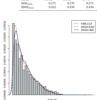
Fig.7. HistogramofobservedEADandpredictedEADdensitiesfrom10-foldcross validationforFRR-CCF,ZAGA-EADandZAGA-USEmodels.

Table7

CoxproportionalhazardsPDmodelcomponentofSurvivalEADmodelona rep-resentativetrainingsample.

Creditusage(percent) 0.239 0.038 <0.001 Ratingclass1vs4 −0.527 0.081 <0.001 Ratingclass2vs4 −0.635 0.039 <0.001 Ratingclass3vs4 −0.315 0.041 <0.001 Averagedaysdelinquent(last3months) 0.007 0.002 <0.001 Averagedaysdelinquent(last12months) −0.020 0.003 <0.001 Relativechangedrawn(last3months) −2.6e−6 1.1e−6 0.021 Absolutechangedrawn(last3months) 4.4e−5 1.3e−5 0.001

(bestperformance).Amongallmodels,theOLS-EADhadthe high-est MAE (worst performance). Although the RMSE was higher thanfor two of theCCF models,ZAGA-EAD hadthe lowest MAE and MAEnorm at 833.5 and 0.268, respectively, among all

non-segmented models. Segmentation by credit usage, i.e. using the OLS-USEand ZAGA-USE approach,reduced the MAE further. The ZAGA-USEhadthelowestMAEofallmodelapproacheswith819.2. Fig.7showstheobservedEADhistogramalongwithﬁttedEAD densitiesforFRR-CCF,ZAGA-EADandZAGA-USE.The ﬁttedvalues

were computedthrough 10-fold crossvalidation.Importantly, the ZAGA-EADmodelisabletoreproducethelargepeakatthelower boundofEAD morecloselythantheother models.Thisalso pro-videsaplausibleexplanationastowhyZAGA-EADwas character-ized by ahighly competitive MAEbuta somewhat disappointing RMSE,asproducingawiderdistributionmayresultinsomelarger residualsthatareheavilypenalizedbythelattercriterion. 4.5. Survivalmodelcomponent

AsurvivalmodelwastrainedtoshowhowanEADmodel hav-ing time todefaultasa covariate could stillbe applied ina pre-diction setting.The resultsofﬁttingtheCox proportionalhazards modelontoarepresentativetrainingsampleareshowninTable7. Positivecoeﬃcientestimatesimplythataunitincreaseinthe vari-ableisassociatedwithanincreasedhazard(andthusshortertime to default)and, conversely,negativevalues indicatereduced haz-ardsofdefaulting(defaulttendstooccurlater).

TheestimatedsurvivalprobabilitiesproducedbythisCoxmodel were then combined with: the ZAGA-EAD model described in Section 3.1; ZAGA-USE, i.e. the best performing segmentation model(cf.Section 3.4);severalofthecompetingCCF modelsand the UTIL model, against which both ZAGA models were bench-markedintheprevioussection.Foreach resultingmodel conﬁgu-ration,predictedEADvalueswerecomputedaccordingtoEq.(15), i.e. by weighting the EAD estimates produced for different de-faulttimeintervalsbythemonthlyPDestimatesfromthesurvival component. As all accounts were guaranteed to defaultwithin a 12 month time horizon, the estimated survival function was set to zero att₌12, i.e.no accountssurvived beyond 12 months in the sample. Each such model combination (referred to as Cox-ZAGA, Cox-ZAGA-USE,Cox-Tobit-CCF, Cox-FRR-CCF,and Cox-Tobit-UTIL, respectively) is a particular instance of the Survival EAD modeldescribedinSection3.5.Thisapproacheliminatestheneed foranypriorknowledgeoftime todefault, andthus allowsusto verifywhethertheperformance improvements obtainedwiththe ZAGAapproachesaremaintainedinapracticaldeploymentsetting where forward-lookingpredictions are required.Table 8 provides the modelperformance comparison forall such selected Survival EADmodelconﬁgurations.

The Cox-ZAGA model demonstrated good discrimination abil-itywithaPearson rof0.798andSpearman

ρ

of0.741.TheMAE andMAEnorm were830.3and0.266.TheRMSEandRMSEnorm were Table8

Performancemeasuresfrom10-foldcrossvalidationforSurvivalEADmodelsusingPDweightingmethod ofEq.(15).

Measure Cox-Tobit-CCF Cox-FRR-CCF Cox-Tobit-UTIL Cox-ZAGA Cox-ZAGA-USE

Pearsonr 0.792 0.792 0.801 0.798 0.798 Spearmanρ 0.721 0.723 0.733 0.741 0.736 MAE 908.8 903.5 1176.2 830.3 860.1 RMSE 1617.5 1615.2 1865.3 1603.2 1593.4 MAEnorm 0.287 0.286 0.375 0.266 0.273 RMSEnorm 0.437 0.437 0.497 0.455 0.435

(10)

1603.2and0.455.Theseresultsshowedverycompetitive explana-torypowercomparedtoasettingwheretime todefaultwouldbe allowedtoentertheEADcalculationdirectly.Infact,thiscombined model,whichdoesnotrelyontimetodefault,performedbetterin terms ofMAEthan mostoftheprevious modelcomponents that usedobservedtimetodefault,exceptforthesegmentedcredit us-age models (see Table 6). Furthermore,Table 8 corroboratesour earlierﬁndingsbyshowingbothZAGAmodelcombinations(cf.the tworight-mostcolumns)stilloutperformedthecompetingmodels intermsofMAE.

5. Conclusionsandfutureresearch

Our study considered the development of EAD models which target the EAD distribution directly in lieuof the CCF.Two such direct models were developed using OLS and the zero-adjusted gammaapproach.Thesewerecomparedtomorecommonlyknown CCF variants using OLS, Tobit and fractional response regression and the utilization change model. Segmentation by credit usage wasalsoattempted,whichinvolvescombiningCCFanddirectEAD modelsbasedonasuitablecut-off level.

ThecrossvalidateddiscriminationmeasuresreportedinTable6 broadly showed that direct EAD models and CCF models risk ranked similarly. In terms of calibration measures (the MAE, MAEnorm,RMSEandRMSEnorm),theFRR-CCFmodelhadthe

high-estperformanceamongCCFvariants.TheOLS-EADmodelhadthe lowestRMSE;however,themodelproduced15negativeﬁtted val-uesofEADasits outputisnotconstrainedtobe apositivevalue. Although thesevalues could intheory be truncated, this maybe considered a drawbackofusing theOLS modelfortargetingEAD directly. The OLS-CCFmodel had the second lowest MAEamong CCF models butitalso produced10 negativeﬁttedvalues ofCCF predictions below zero.The utilization changemodel, Tobit-UTIL, didnotperformaswellastheothermodels.

When comparing the non-segmented models, the ZAGA-EAD showed the highestperformance amongthe CCF anddirect EAD models, havingthelowest MAEandMAEnorm fromthecross

val-idated ﬁndings (see Table 6). Additionally, the ZAGA-EAD model doesnotproducenegativeEADvaluesasthezero-adjustedgamma distributiononlypredictsvaluesofzeroandabove.

The notion that CCF modelsperform better forlow credit us-ageaccountsandthat directEADmodels performbetter forhigh credit usage accounts appeared to be supported by various ﬁnd-ings.Thepositiverelationshipoftheundrawnpercentagewiththe dispersion parameter in the ZAGA-EAD model indicated that di-rect EADmodels providelesspreciseestimatesforlowcredit us-age.Also, thesegmentedcredit usagemodels developedby com-bining CCF and direct EAD models provided further performance improvements (see Table 6). Although the discrimination results remained broadly similar relative to non-segmented models, the calibrationperformancewasimprovedwithlower MAEandRMSE valuesobservedforbothtypesofsegmentedmodels.TheOLS-USE model produced thesecond lowest MAEamong all modeltypes; the ZAGA-USEmodelhadthe lowestMAEwhich representedthe mostaccuratemodelforthisstudy.

OurmodelsfromTable6includedtheobservedtimetodefault asapredictivecovariate.Weshowedthatthetimetodefault vari-able,whichisunknown aprioriforacreditline,cannonetheless beappliedinapredictioncontextbyusingasurvivalmodel com-ponentalongsideadirectEADmodelapproach.ThisprovidesEAD estimatesforeachmonthweightedbytherespectivePD.According toTable8,theSurvivalEADmodelswerecompetitiveandhad sim-ilar performance comparedto the use ofa model withobserved values oftime todefault. When combinedwiththe weightedPD approach,theCox-ZAGA-EADmodelhadthelowestMAEwhilethe Cox-ZAGA-USEmodelhadthesecond lowestMAEandthelowest

RMSE.Inotherwords,theZAGA approachproved highly competi-tive,notjustwithobservedtimeofdefaultbutequallywhen com-binedwithasurvivalmodelcomponentthatdoesnotrequireprior knowledgeofthisvariable.

The direct EAD models had some limitations with respect to drawnbalances.BaselcompliancerequiresestimatedEADtobeat leastequaltoorabovethedrawnbalanceofthecreditline.Some accountsfromdirectEAD modelscouldhavepredictedavalue of EADthat is lessthan thedrawn balance. Thus duringmodel im-plementation, appropriate overrides could be used to floor such account-levelEADpredictionsattheobserveddrawnbalance.This effectwould not occur fortruncated CCF models where the CCF cannot take values below zero.We note however that if the di-rect EAD model is used to pool accounts intodifferent EAD risk grades,account-levelestimatesofEADthatfall outsideofthe ex-pectedrangewouldpresentlessofa problemandtheZAGA-EAD model’s better calibration performance would likely implybetter grade-levelestimatesofEAD.However, thedirectEADmodelsare morecomplexwithmoreparameterstoestimate;hence,forusein industry,modeldevelopersshouldconsider potentialimplications ofthislevelofcomplexityformodelimplementationandauditing. Future avenues for research could explore further improving thesegmentedcreditusagemodelsbyconsideringalternativeCCF model components, for example, using a beta inflated mixture model (Rigby & Stasinopoulos, 2010) to accommodate the highly bimodal nature of the CCF distribution. Other EAD distributions withlongtails mayalsobe tried aspartofthe directEAD mod-els,e.g.usingtwocomponentgammadistributionsfortwo under-lying subpopulationsof low andhighEAD amounts. Thesurvival modelcomponentmaybefurtherdevelopedusingparametric sur-vivalmodelswithtruncatedsurvivaldistributionswhichallowsfor fixedmaximumtimehorizonsgivendefaultedaccountshavedone sowithina12monthhorizon.

In summary,our results suggest direct EAD models using the gammamodelwithouttheCCFformulationofferacompetitive al-ternative toCCF orutilizationchange basedmodels. Theﬁndings alsoindicatemodelsegmentationbycreditusagemayimprove cal-ibrationperformancefurther,whichimpliesdirectEADmodelsare acomplementto CCFbased models.Thisis apositive ﬁndingfor EADmodelsasthefocusofpredictionisnotonlyonrisk ranking abilitybutontheconcordanceoftheobservedandpredicted val-ues.WesuggestEADmodeldevelopersconsiderexploringtheuse ofdirectEADmodelsandcreditusageasasegmentationcriterion forupliftincalibrationperformanceandtoimproverisksensitivity ofcreditriskmodels.

Acknowledgements

We thank several anonymous reviewers, as well as Professor Joe Whittaker (University of Lancaster) and Dr. Katarzyna Bijak (UniversityofSouthampton)fortheirrecommendationswhich im-provedthemanuscript.

References

Akaike,H.(1974).Anewlookatthestatisticalmodelidentiﬁcation.IEEE Transac-tionsonAutomaticControl,19,716–723.

BaselCommitteeonBankingSupervision(2005).Internationalconvergenceof capi-talmeasurementandcapitalstandards:Arevisedframework.Basel,Switzerland: BankforInternationalSettlements.

BaselCommitteeonBankingSupervision(2011).BaselIII:Aglobalregulatory frame-workformoreresilientbanksandbankingsystems.Basel,Switzerland:Bankfor InternationalSettlements.

Bellotti,T.,&Crook,J.(2012).Lossgivendefaultmodelsincorporating macroeco-nomicvariablesforcreditcards.InternationalJournalofForecasting,28,171–182. Bijak,K.,&Thomas,L.C.(2015). ModellingLGDfor unsecuredretailloansusing

Bayesianmethods.JournaloftheOperationalResearchSociety,66,342–352. Brown,I.(2011). Regressionmodeldevelopmentforcredit cardexposure atdefault

(EAD)usingSAS/STAT® _and _SAS® _Enterprise _MinerTM _5.3_. _Las _Vegas,_NV: _SAS GlobalForum.

(11)

Brown,I.L.J.(2014).DevelopingcreditriskmodelsusingSASenterpriseminerand SAS/STAT:Theoryandapplications.Carey,NC:SASInstitute.

Cox,D.R.(1972).Regressionmodelsandlife-tables.JournaloftheRoyalStatistical Society:SeriesB(Methodological),34,187–220.

Eilers,P.H.C.,&Marx,B.D.(1996).FlexiblesmoothingwithB-splinesandpenalties.

StatisticalScience,11,89–102.

Greene,W.H.(1997).Econometricanalysis.London:PrenticeHallInternational. Hastie,T.,Tibshirani,R.,&Friedman,J.(2009).Theelementsofstatisticallearning:

Datamining,inference,andprediction.NewYork,NY:Springer.

Hosmer,D., Lemeshow,S., &May,S.(2008). Appliedsurvivalanalysis:Regression modelingoftimetoeventdata.Wiley-Interscience.

Jacobs,M.,Jr.(2010).Anempiricalstudyofexposureatdefault.JournalofAdvanced StudiesinFinance,1,31–59.

Leow,M.,&Crook,J.(2015).Anewmixturemodelfortheestimationofcreditcard exposureatdefault.EuropeanJournalofOperationalResearch,249(2),487–497. Loterman,G.,Brown,I.,Martens,D.,Mues,C.,&Baesens,B.(2012).Benchmarking

regression algorithmsfor lossgivendefaultmodeling.InternationalJournalof Forecasting,28,161–170.

Malik,M.,&Thomas,L.(2010).Modellingcreditriskofportfolioofconsumerloans.

JournaloftheOperationalResearchSociety,61,411–420.

Mccullagh,P.,&Nelder,J.A.(1989).Generalizedlinearmodels.NewYork:Chapman andHall.

Moral,G.(2011).EADestimatesforfacilitieswithexplicitlimits.InB.Engelmann, &R.Rauhmeier(Eds.),TheBaselIIriskparameters:Estimation,validation,stress testing– withapplicationstoloanriskmanagement(2nded).Berlin:Springer. Nelder,J.A.,&Wedderburn,R.W.M.(1972).Generalizedlinearmodels.Journalof

theRoyalStatisticalSociety:SeriesA(General),135,370–384.

Papke,L.E., &Wooldridge,J.M.(1996).Econometric methodsfor fractional re-sponsevariableswithanapplicationto401(k)planparticipationrates.Journal ofAppliedEconometrics,11,619–632.

Qi,M.(2009).Exposureatdefaultofunsecuredcreditcards.Economicsworkingpaper 2009-2.OﬃceoftheComptrolleroftheCurrency.

Qi,M.,&Zhao,X.(2011).Comparisonofmodelingmethodsforlossgivendefault.

JournalofBanking&Finance,35,2842–2855.

Rigby,R.A.,&Stasinopoulos,D.M.(2005).Generalizedadditivemodelsforlocation, scaleandshape.JournaloftheRoyalStatisticalSocietySeriesC,54,507–554. Rigby,R.A.,&Stasinopoulos,D.M.(2007).Generalizedadditivemodelsforlocation

scaleandshape(GAMLSS)inR.JournalofStatisticalSoftware,23,1–46.

Rigby, R.A. & Stasinopoulos, D.M. (2010). A ﬂexible regression approach us-ing GAMLSS in R. http://www.gamlss.org/wp-content/uploads/2013/01/ book-2010-Athens1.pdf

So,M.C.,Thomas,L.C.,Seow,H.-V.,&Mues,C.(2014).Usingatransactor/revolver scorecardtomakecreditandpricingdecisions. DecisionSupportSystems,59, 143–151.

Stepanova,M., &Thomas,L. (2002).Survival analysismethodsfor personalloan data.OperationsResearch,50,277–289.

Taplin,R.,MinhTo,H.,&Hee,J.(2007).Modelingexposureatdefault,credit con-versionfactorsandtheBaselIIaccord.TheJournalofCreditRisk,3,75–84. Tobin,J.(1958).Estimationofrelationshipsforlimiteddependentvariables.

Econo-metrica,26,24–36.

Tong,E.N.C.,Mues,C., &Thomas,L.(2013).A zero-adjustedgammamodelfor mortgageloanlossgivendefault.InternationalJournalofForecasting,29,548– 562.

Tong,E.N.C.,Mues,C.,&Thomas,L.C.(2012).Mixturecuremodelsincredit scor-ing:Ifandwhenborrowersdefault.EuropeanJournal ofOperationalResearch, 218,132–139.

Valvonis,V.(2008).EstimatingEADforretailexposuresforBaselIIpurposes.The JournalofCreditRisk,4,79–109.

Witzany,J.(2011).Exposureatdefaultmodelingwithdefaultintensities.European FinancialandAccountingJournal,6,20–48.

Yang,B.H.,&Tkachenko,M.(2012).Modeling exposureat defaultand lossgiven de-fault:Empiricalapproachesandtechnicalimplementation.TheJournalofCredit Risk,8,81–102.