sound diffraction, delay, and reflection. The simplicity of the model permits efficient implementation in DSP hardware, and thus facilitates real-time operation. Additionally, the parameters in the model can be adjusted to fit a particular individual’s characteristics, thereby producing individualized head-related transfer functions. Experimental tests verify the perceptual ef-fectiveness of the approach.
Index Terms—Binaural, head-related transfer functions,
local-ization, spatial hearing, 3-D sound, virtual auditory space.
I. INTRODUCTION
T
HREE-DIMENSIONAL (3-D) sound is becoming in-creasingly important for scientific, commercial, and en-tertainment systems [1]–[3]. It can greatly enhance auditory interfaces to computers, improve the sense of presence for virtual reality simulations, and add excitement to computer games. Current methods for synthesizing 3-D sound are either simple but limited, or complicated but effective. We present a modeling approach that promises to be both simple and effective.It is well known that the physical effects of the diffraction of sound waves by the human torso, shoulders, head and outer ears (pinnae) modify the spectrum of the sound that reaches the ear drums [4], [5]. These changes are captured by the head-related transfer function (HRTF), which not only varies in a complex way with azimuth, elevation, range, and frequency, but also varies significantly from person to person [6], [7]. The same information can also be expressed in the time domain through the head-related impulse response (HRIR), which reveals interesting temporal features that are hidden in the phase response of the HRTF.
Strong spatial location effects can be produced by con-volving a monaural signal with HRIR’s for the two ears and either presenting the results through properly compensated headphones [8] or through cross-talk-canceled stereo speakers Manuscript received September 7, 1996; revised August 20, 1997. This work was supported by the National Science Foundation under Grant IRI-9214233. Any opinions, findings, and conclusions or recommendations ex-pressed in this paper are those of the authors and do not necessarily reflect the views of the National Science Foundation. The associate editor coordinating the review of this manuscript and approving it for publication was Dr. Dennis R. Morgan.
C. P. Brown is with the Department of Electrical Engineering, University of Maryland, College Park, MD 20742 USA (e-mail: cpbrown@isr.umd.edu). R. O. Duda is with the Department of Electrical Engineering, San Jose State University, San Jose, CA 95192 USA (e-mail: duda@best.com).
Publisher Item Identifier S 1063-6676(98)05938-0.
finite impulse response (FIR) filter coefficients derived from experimentally measured HRIR’s and indexed by azimuth and elevation [2]. Furthermore, to produce the most convincing elevation effects, the HRIR must be measured separately for each listener, which is both time consuming and highly inconvenient.
To simplify spatial audio systems, several researchers have proposed replacing measured HRIR’s with computational models [9]–[11]. Azimuth effects (or, more properly, later-alization effects) can be produced merely by introducing the proper interaural time difference (ITD). Adding the appropriate interaural level difference (ILD) improves the coherence of the sound images. Introducing notches into the monaural spectrum creates definite elevation effects [12], [13]. However, there are major person-to-person variations in elevation perception, and the effects are very difficult to control. In addition, sounds in front frequently appear to be too close, and front/back reversals are not uncommon.
In this paper, we present a simple and effective signal processing model of the HRIR for synthesizing binaural sound from a monaural source. The components of the model have a one-to-one correspondence with the shoulders, head, and pin-nae, with each component accounting for a different temporal feature of the impulse response. Thus, our model is developed primarily in the time domain.
The question of whether it is better to model in the fre-quency domain or the time domain is an old debate that is not easily settled. Of course, the two domains are mathematically equivalent, so that a model that captures the time-domain response without error also captures the frequency-domain response without error. The problem is that any model will introduce error, and the relation between time-domain and frequency-domain errors is not always clear.
Psychoacoustically, critical-band experiments show that the ear is usually not sensitive to relative timing or phase, as long as the signal components lie in different critical bands [14]. In particular, it is not possible to discriminate monaurally between the temporal order of events that occur in intervals shorter than 1–2 ms [15]. These kinds of observations lend support to Helmholz’s conclusion that the ear is “phase deaf,” and have caused most researchers to favor frequency-domain modeling [11]. However, the ear can discriminate interaural time differences that are as short as 10 s [14]. Thus, when different models are developed for the two ears, it is important 1063–6676/98$10.00 1998 IEEE
BROWN AND DUDA: BINAURAL SOUND SYNTHESIS 477
to control the time-domain as well as the frequency-domain errors.
However, our primary reason for focusing on the time domain is that many of the characteristics of HRTF’s are a consequence of sound waves reaching the ears by multiple paths. Signals that arrive over paths of very different lengths interact in ways that are obscure in the frequency domain, but are easy to understand in the time domain. This greatly simplifies the process of determining the structure of the model. Ultimately, the final test is the degree to which the model correctly captures spatial information as revealed by psychoacoustic testing.
We begin by reviewing the physical basis for the HRIR. We first consider the low-frequency effects of the head alone, and then investigate the effects of the shoulders and pinnae. In each case, we present a simple signal processing model that captures major temporal features of the HRIR. The model is parameter-ized to allow for individual variations in size and shape. We then present the results of testing three subjects to see how well their individualized models compare to their measured HRIR’s in localizing sounds. Here we focus on the difficult problem of elevation estimation, but we simplify the situation by restricting ourselves to sources in front of the listener. We conclude with some observations on unsolved problems.
II. SOUNDDIFFRACTION AND THE HRTF A. Rayleigh’s Spherical Model
While it is theoretically possible to calculate the HRTF by solving the wave equation, subject to the boundary conditions presented by the torso, shoulders, head, pinnae, ear canal, and ear drum, this is analytically beyond reach and computationally formidable. However, many years ago Lord Rayleigh obtained a simple and very useful low-frequency approximation by deriving the exact solution for the diffraction of a plane wave by a rigid sphere [16]. The resulting transfer function
gives the ratio of the phasor pressure at the surface of the sphere to the phasor free-field pressure [17]. Here is the radian frequency and is the angle of incidence, the angle between a ray from the center of the sphere to the sound source and a ray from the center of the sphere to the observation point. Because the results scale with the radius , they are usually expressed in terms of the normalized frequency given by
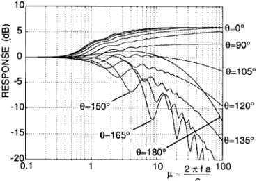
(1) where is the speed of sound (approximately 343 m/s). For the commonly cited 8.75-cm average radius for an adult human head [17], corresponds to a frequency of about 624 Hz. Normalized amplitude response curves for Rayleigh’s solu-tion are shown in Fig. 1. These results account for the so-called “head shadow,” the loss of high frequencies when the source is on the far side of the head. For binaural listening, the phase response is even more important than the amplitude response. The properties of the phase and group delay for a sphere are reviewed by Kuhn [17]. For , the difference between the time that the wave arrives at the observation point and the time it would arrive at the center of the sphere in free
Fig. 1. Frequency response of an ideal rigid sphere (f = frequency, a = radius,c = speed of sound). Note that the response drops off with the angle of incidence up to about 150, and then rises again to the “bright spot” at 180. space is well approximated by Woodworth and Schlosberg’s frequency-independent formula [4], which we write as
if if
(2)
However, for the relative delay increases beyond this value, becoming approximately 50% greater than the value predicted by (2) as [17].
B. An Approximate Spherical-Head Model
As a first-order approximation, one can model an HRTF by simple linear filters that provide the relative time delays specified by (2). This will provide useful ITD cues, but no ILD cues. Furthermore, the resulting ITD will be independent of frequency, which is contrary to Kuhn’s observations [17]. Both of these problems can be addressed by adding a minimum-phase filter to account for the magnitude response. We have obtained useful results by cascading a delay element corre-sponding to (2) with the following single-pole, single-zero head-shadow filter:
(3)
where the frequency is related to the radius of the sphere by (4) The normalized frequency corresponding to is
. The coefficient , which is a function of the angle of incidence , controls the location of the zero. If , there is a 6 dB boost at high frequencies, while if there is a cut. To match the response curves shown in Fig. 1, one must relate to . As Fig. 2 illustrates, the choice
(5)
Fig. 2. Frequency response of a simple one-pole-one-zero spherical-head model [cf., Fig. (1)]. The pole is fixed at = 2, and the zero varies with the angle of incidence.
good approximation to the ideal solution shown in Fig. 1. Furthermore, note that at low frequencies also introduces
a group delay , which
adds to the high-frequency delay specified by (2). In fact, at the head-shadow filter provides exactly the 50% additional low-frequency delay observed by Kuhn [17]. Thus, a model based on (2)–(5) provides an approximate but simple signal processing implementation of Rayleigh’s solution for the sphere.
C. Experimental Procedure
Because there is no theoretical solution to the more compli-cated diffraction effects produced when sound waves strike a human listener, all of the results in the rest of this pa-per come from expa-perimental measurements. The expa-periments
were made in a 2 2 2.4 m anechoic chamber at
San Jose State University. The measurements were made with the Snapshot system built by Crystal River Engi-neering. This system uses computer-generated Golay codes [18] to excite a Bose Acoustimass loudspeaker. The acoustic signals were picked up either by two Etymotic Research ER-7C probe microphones or by two small Panasonic blocked-meatus microphones intended to be inserted into a human subject’s ear canals. Although blocked-meatus microphones disturb the boundary conditions and cannot capture the ear-canal resonance, it is generally believed that they capture the directionally dependent components of the HRTF [19].
The standard Snapshot system uses minimum-phase recon-struction to obtain shorter, time-aligned impulse responses. However, it also provides access to the unprocessed impulse responses through its “oneshot” function. This was used to obtain the impulse response for the chain consisting of the D/A converter, amplifier, loudspeaker, microphones, and A/D converter. Sampling was done at 44.1 kHz, with a signal-to-noise ratio in excess of 70 dB. The record length was 256 samples, or about 5.8 ms, which provided a frequency resolution of 172 Hz. All impulse responses decayed to less than 1% of their peak values in less than 2.5 ms.
Fig. 3. The interaural polar coordinate system. Note that a surface of constant azimuth is a cone of basically constant interaural time difference. Also, note that it is elevation, not azimuth, that distinguishes front from back.
To provide reference data, the free-field responses were measured with the microphones suspended in the empty cham-ber. A minimum-phase reconstruction showed that the free-field responses were essentially minimum-phase, and their inverses were stable. At high frequency, these free-field re-sponses were relatively flat: dB in the range from 2–20 kHz. Below 2 kHz, there was a steady 6-dB/octave rolloff, due primarily to the loudspeaker. While that made it difficult to compensate the response below 200 Hz, no more than 30-dB correction was required for the range from 200–20 kHz. Free-field compensation of the response measurements was done by windowing the free-field response, dividing the FFT of a measured impulse response by the FFT of the windowed free-field response, and inverse transforming the results. This operation cannot be done at DC, where the speaker provides no energy at all. Because any measured response must approach the free-field response as the frequency approaches zero, we corrected the resulting frequency responses by setting the DC values to unity before the inversion.
D. KEMAR Impulse Responses
Many studies of HRTF’s have used the acoustic manikin, Knowles Electronics Manikin for Acoustic Research (KE-MAR). [17], [20], [21]. KEMAR has the advantage over other dummy heads of having a torso and detachable pinnae. As Kuhn has demonstrated, by removing the pinnae one can see the effect of the torso and the nonspherical head, and by remounting the pinnae one can see the modifications that the pinnae introduce [21].
KEMAR was mounted on a pipe that could be rotated about its vertical axis. The source was located relative to the head using the head-centered interaural-polar coordinate system shown in Fig. 3. For a source in the horizontal plane, azimuths of 0 , 90 , or 90 correspond to a sound coming from the front, the right side, or the left side, respectively. KEMAR was equipped with the so-called “small orange pinnae.” When the pinnae were removed, the resulting cavities were filled in and the probe microphone was placed inside the head, with the opening of probe tube flush with the head surface. When the pinnae were attached, the ear canals were blocked with modeling clay, so that the results could be directly
BROWN AND DUDA: BINAURAL SOUND SYNTHESIS 479
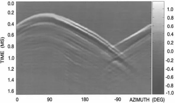
Fig. 4. Image representation of the impulse response of the right ear of the KEMAR manikin without pinna. Each column is an impulse response, where brightness corresponds to value according to the scale at the right. Note the shoulder reflection that occurs about 0.35 ms after the main pulse. Note also the bright spot around0100 azimuth where the waves traveling around the front and back meet.
compared with subsequent blocked-meatus measurements of human subjects. The probe microphone was taped to the top of the head above the ear, with the opening of the probe tube at the center of the entrance to the blocked ear canal. The Snapshot system was used to make a series of impulse response measurements. The loudspeaker was directed at the center of KEMAR’s head at a distance of 1 m, and KEMAR was rotated in 5 increments between measurements.
Head shadow caused the impulse response for the right ear to be large for azimuths near 90 and small for azimuths near 90 . To compensate for the loss of high frequencies on the shadowed side, we filtered the responses with the inverse of the head-shadow filter given by (3). The resulting impulse responses are presented as an image in Fig. 4. Each column in the image corresponds to an impulse response at a particular azimuth, and each row corresponds to a moment in time. The gray level of a pixel representing the value of the response is in accordance with the intensity scale at the right side of the image. The arrival of the main pulse is clearly seen as the bright arc at the top of the image. The time delay, which closely follows (2), is smallest near the right ear location at 100 , and largest around the left-ear location at 100 . Between 80 and 100 the impulse response is more complicated, as waves around the front of the head and around the back of the head combine. Although HRTF’s are generally minimum-phase [6], a minimum-phase reconstruction of the impulse response indicates that the HRTF is not minimum-phase in this range; the perceptual importance of this observation is unknown.1
1In general, the perceptual significance of particular visual features in the
HRIR images is unclear. Many visual patterns can be seen, but it is hard to say whether or not the auditory system is sensitive to them. Conversely, aspects of the HRIR that are important for auditory perception may be hidden by such a visual representation. Nevertheless, we find image displays useful to identify general trends in the data and to hypothesize models. Auditory
Between 20 and 180 , one can also see a faint echo that arrives about 0.35 ms after the main pulse. This delay time corresponds to a path length difference of 13 cm, which is consistent with a shoulder reflection; the fact that the echo is most prominent in the azimuth range where the shoulder is most strongly “illuminated” also supports that interpretation.
Addition of the pinna introduces new complexity into the impulse responses. Fig. 5 shows the impulse responses after compensation for head shadow. The pinna introduces a series of strong additional ridges. Over much of the range the initial pulse is followed about 60–80 s later by a strong second pulse. This also shows up in the spectrum as a sharp null or notch in the 8–6-kHz range. Although the detailed physical behavior of the pinna is quite complex [22], it is tempting to interpret these ridges either as echoes or resonances. Batteau [23] proposed a simple two-echo model of the pinna that produced elevation effects in subsequent psychoacoustic tests by Watkins [13]. However, the pinnae primarily influence the response at high frequencies, and when the wavelength approaches the physical size of diffracting objects, describing its behavior in terms of reflections or echoes becomes problematic [4], [5], [22].
E. Elevation Effects of the Pinna
Although the pinna provides some azimuth information, it has been studied primarily because of its importance for elevation estimation. In measuring elevation, most researchers employ a vertical-polar spherical coordinate system. However, we prefer the interaural-polar system, because in that system surfaces of constant azimuth are cones of essentially constant interaural time difference (see Fig. 3). Here the azimuth is restricted to the interval from 90 to 90 , while the tests are required to determine the validity of these models.
Fig. 5. Impulse response of the right ear of the KEMAR manikin with pinna. The splitting of the initial pulse into a pair of pulses shows up in the spectrum as a notch in the 6 to 8 kHz range. The multiple ridges can be interpreted as multiple “echoes” or as resonances in the pinna cavities.
Fig. 6. Elevation dependence of the HRIR for the median plane ( = 0) for a human subject. Note that arrival times of the “pinna echoes” increase as the source moves from overhead to below. The fainter echoes that have the opposite trend are due to shoulder and torso reflection.
elevation ranges over the full interval from 180 to 180 . This means that with interaural-polar coordinates, it is elevation rather than azimuth that distinguishes front from back. For simplicity, we restricted all of our measurements on human subjects to the frontal half space, so that the elevation was also restricted to the interval from 90 to 90 .
To measure the elevation variation of the HRIR, the loud-speaker was mounted on a fixture that allowed it to be pointed directly at the center of the head and rotated about an axis aligned with the interaural axis. The subjects were seated with
the blocked-meatus microphones inserted in their ear canals, using ear ring seals to block the ear-canal resonance and to keep the microphones in place. Measurements were taken at 5 increments for three human subjects, identified as PB, RD, and NH. As expected, the arrival times for these measurements were essentially the same for all elevations.
Fig. 6 shows how the left-ear impulse response for PB varies with elevation in the median plane ( ). In this and in all subsequent images, the responses were free-field corrected and compensated for head shadow. In addition, to remove
BROWN AND DUDA: BINAURAL SOUND SYNTHESIS 481
Fig. 7. A schematic representation of the major features in the impulse response image. These define what are called the “pinna events.”
the effects of timing differences due to small head motions and/or positioning inaccuracies, the individual impulse re-sponses were interpolated by a factor of four and time aligned. Time alignment not only removed distracting wiggles from the images, but also greatly simplified comparisons between different cases.
Because the physical interpretation of pinna elevation cues is somewhat controversial, we shall refer to the ridges and troughs that can be seen in the impulse response as “events.” After examining many images like Fig. 6, we adopted a standard way to describe them in terms of the schematic characteristics depicted in Fig. 7. The initial ridge is followed by a sequence of ridges and troughs. These features are similar to the envelope peaks observed by Hiranaka and Yamasaki [24], who noted that a source in front produces two or more major reflections, which fuse with the main pulse as the elevation approaches 90 . In Fig. 6, a second ridge occurs roughly 50 s after the initial ridge and varies only slightly with elevation. It is followed by a very prominent trough and ridge pair whose latency varies nearly monotonically
with elevation from about 100 s at to 300 s
at . The sharply positive sloping diagonal events are due to a shoulder reflection and its replication by pinna effects. Other fainter patterns can often be seen, perhaps due to resonances of the pinna cavities (cavum concha and fossa), or to paths over the top of the head and under the chin. The importance of these weaker events remains unclear.
Fig. 8 shows time-aligned impulse responses for both the contralateral and ipsilateral ear (far and near ear) for five different azimuth angles. As one would expect from the geometry, the shoulder echoes vary significantly with azimuth. The pinna events also exhibit some azimuth dependence, but it is not pronounced. It is particularly interesting that the tim-ing patterns, includtim-ing the azimuth variation, are remarkably similar for the ipsilateral and the contralateral ears.
III. HRIR AND HRTF MODELS A. The Problem
The HRIR and the HRTF are functions of four vari-ables—three spatial coordinates and either time or frequency. Both functions are quite complicated, and they vary signifi-cantly from person to person. As we mentioned earlier, the most effective systems for 3-D sound synthesis have stored large tables of FIR filter coefficients derived from HRIR measurements for individual subjects. The desirability of replacing such tables by functional approximations has been recognized for some time [11]. In principle, this is merely a problem in system identification, for which there are well known standard procedures. However, four major problems complicate the system identification task.
1) It is difficult to approximate the effects of wave propaga-tion and diffracpropaga-tion by low-order parameterized models that are both simple and accurate.
2) The HRIR and HRTF functions do not factor, resulting in strong interactions between the four variables. If the model parameters vary with spatial location in such a complex way that they themselves must be stored in large tables, the advantages of modeling are lost. 3) There is no quantitative criterion for measuring the
ability of an approximation to capture directional infor-mation that is perceptually relevant.
4) An approximation that works well for one individual may not work well for another. Thus, it may be nec-essary to solve the system identification repeatedly for each listener.
This last problem might not be too serious in practice, since it may well be possible to treat HRTF’s like shoes, providing a small number of standard “sizes” from which to choose [25]. The lack of an objective error criterion is more troubling. There is no reason to believe that a model that seems to do
(a)
(b)
Fig. 8. Azimuth dependence of the head-related impulse response. (a) Far ear, head-shadow removed. (b) Near ear. Unlike the shoulder reflection, the events that arrive early do not vary much with azimuth in this range of azimuths. A faint “parabolic” reflection seen in the far ear around 30 azimuth is conjectured to be due to the combination of waves traveling over the top of the head and under the chin.
well at matching visually prominent features or that minimizes mean square error in either the time or the frequency domains will also produce perceptually convincing effects. Many re-searchers have attempted to identify those characteristics of the HRTF that control spatial perception (see [4], [5], and refer-ences therein). Fewer researchers have explored the HRIR, and they have primarily been concerned with localization in the median plane [23], [24], [26]. The perceptual effects of time-domain errors are far from clear. Thus, the only currently avail-able way to evaluate a model is through psychoacoustic tests.
To date, three different approaches have been taken to devel-oping models: 1) rational-function approximations (pole/zero models) plus time delay; 2) series expansions; and 3) structural models. We consider each of these in turn.
B. Pole/Zero Models
The head-shadow filter given by (3) is a particularly simple example of a rational function approximation to an HRTF. Indeed, we include it in the model that we propose. Used all by itself, it can produce fairly convincing azimuth effects, even
BROWN AND DUDA: BINAURAL SOUND SYNTHESIS 483
though it matches only the gross magnitude characteristics of the HRTF spectrum. Its effectiveness can be noticeably enhanced by adding an all-pass section to account for propaga-tion delay and thus the interaural time difference. This leads to a head model of the form
(6)
where is obtained by adding to (2) to keep the delays causal, is given by (4), by (5), and where specifies the location of the entrance to the ear canal, e.g.,
100 for the right ear and 100 for the left ear.
Elementary as it is, this model has many of the character-istics that we desire. In listening tests, the apparent location of a sound source varies smoothly and convincingly between the left and right ear as varies between 90 and 90 . It can be individualized by adjusting its four parameters , , , and . Finally, while it does not factor into one function of frequency times another function of azimuth, it is sufficiently simple that real-time implementation is easy.
Of course, this model produces only azimuth effects, while it is well known that individualized HRTF’s can produce both azimuth and elevation effects [27]. To capture both azimuth and elevation cues, we must now contend with a function of three variables, . In evaluating Batteau’s two-echo theory, Watkins showed that merely by changing the time delay in a monaural model of the form
(7) he could produce a spectrum with an appropriately moving notch. His psychoacoustic tests showed that this produced the effect of vertical motion in the frontal plane, at least for elevation angles between 45 and 45 [13]. This and other research on localization in the median plane tended to support a first-order theory that azimuth cues are binaural while eleva-tion cues are monaural [28]. This in turn suggested that it might be possible to factor the HRTF into an azimuth-dependent part and an elevation-dependent part, and models having this structure have been proposed [9]. However, the interaural level difference is both azimuth and elevation dependent [29], and elevation effects produced only by monaural cues tend to be rather weak.
Being unable to factor the problem, researchers have ap-plied various filter design, system identification, and neural network techniques in attempts to fit multiparameter models to experimental data [30]–[37]. Unfortunately, many of the resulting filter coefficients are themselves rather complicated functions of both azimuth and elevation, and models that have enough coefficients to be effective in capturing individual-ized directional cues do not provide significant computational advantages.
C. Series Expansions
Although HRTF’s appear to be complicated, one can argue on a physical basis that they should be completely determined
by a relatively small number of physical parameters—the aver-age head radius, head eccentricity, maximum pinna diameter, cavum concha diameter, etc. This suggests that the intrinsic dimensionality of the HRTF’s might be small, and that their complexity primarily reflects the fact that we are not viewing them correctly.
In the search for simpler representations, several researchers have applied principal components analysis (or, equivalently, the Karhunen–Lo´eve expansion) to the log magnitude of the HRTF [6], [38], or to the complex HRTF itself [39]. This produces both a directionally independent set of basis functions and a directionally dependent set of weights for combining the basis functions. One can also exploit the periodicity of the HRTF’s and use a Fourier series expansion [29]. The results of expanding the log-magnitude can be viewed as a cascade model, and is most natural for representing head diffraction, ear-canal resonance, and other operations that occur in sequence. The results of expanding the complex HRTF can be viewed as a parallel model, and is most natural for representing shoulder echoes, pinna “echoes,” and other multipath phenomena.
In all of these cases, it has been found that a relatively small number of basis functions are sufficient to represent the HRTF, and series expansions have proved to be a valuable tool for studying the characteristics of the data. Furthermore, it may be possible to relate them to anthropometric measurements and to scale them to account for individual differences [40]. Unfortunately, they still require significant computation for real-time synthesis when head motion or source motion is involved, because the weights are relatively complex functions of azimuth and elevation that must be tabulated, and the resynthesized HRTF’s must be inverse-Fourier transformed to obtain the HRIR’s needed to process the signals.
D. Structural Models
A third approach to HRTF modeling is to base it on a sim-plified analysis of the physics of wave propagation and diffrac-tion. Lord Rayleigh’s spherical model can be viewed as a first step in this direction, as can Batteau’s two-echo theory of the pinna and the more sophisticated analysis by Lopez–Poveda and Meddis [41]. The most ambitious work along these lines is the model developed by Genuit [42], [43]. In his thesis research, Genuit identified 34 measurements that characterized the shape of the shoulders, head, and pinnae. To formulate the problem analytically, he approximated the head and pinnae by tubes and circular disks, and he then proposed combining these solutions heuristically to create a structural model.
Genuit’s model has several appealing characteristics. First and foremost, each component is present to account for some well identified and significant physical phenomenon. Second, it is economical and well suited to real-time implementation. Third, it offers the promise of being able to relate filter parameters to anthropometric measurements. Finally, it is neither a cascade nor a multipath model, but rather a structural model that is naturally suited to the problem. The model has been successfully incorporated in a commercial product [44]. However, to the best of our knowledge, it has not been
Fig. 9. A structural model of the head-related transfer function. Separate modules account for head shadow, shoulder reflections, and pinna effects.
objectively evaluated, and its detailed structure has not been revealed.
IV. A STRUCTURAL MODEL A. Structure of the Model
Our observations on the HRIR data suggest an alternative structural model based on combining an infinite impulse response (IIR) head-shadow model with an FIR pinna-echo model and an FIR shoulder-echo model. Our model has the general form shown in Fig. 9. Here the ’s are reflection coefficients and the ’s and ’s are time delays. The rationale for this structure is that sounds can reach the neighborhood of the pinnae via two major paths—diffraction around the head and reflection from the shoulders. In either case, the arriving waves are altered by the pinna before entering the ear canal.
Any such model is an approximation, and can be either refined or further simplified. For example, an examination of the shoulder echo patterns in Fig. 8 reveals that the shoulder reflection coefficients and vary with elevation. Furthermore, since the shoulder echoes arrive at the ear from a different direction than the direct sound, they should really pass through a different pinna model. All of this is further complicated by the fact that these directional relations will change if the listener turns his or her head. Fortunately, informal listening tests indicated that the modeled shoulder echoes did not have a strong effect on the perceived elevation of a sound, and we actually decided to omit the shoulder-echo component from our evaluation tests.
Carlile [5] divides pinna models into three classes: res-onator, reflective, and diffractive. Our model can be described as being reflective, but we allow negative values for two of the pinna reflection coefficients, which might correspond to a longitudinal resonance. These coefficients and their corre-sponding delays vary with both azimuth and elevation. For a symmetrical head, the coefficients for the left ear for an azimuth angle should be the same as those for the right ear for an azimuth angle . Although the pinna events definitely depend on azimuth, we were somewhat surprised to find that their arrival times were quite similar for the near and the
far ear (see Fig. 8). If this were also true for the reflection coefficients, it would imply that the ILD is independent of elevation, which is not the case [29]. Thus, differences in the pinna parameters are needed to account for the variation of the ILD with elevation.
B. Parameter Values
Examination of the impulse responses indicated that most of the pinna activity occurs in the first 0.7 ms, which corresponds to 32 samples at a 44.1-kHz sampling rate. Thus, a single 32-tap FIR filter was selected for the elevation model. Six pinna events were deemed to be sufficient to capture the pinna response. There are two quantities associated with each event, a reflection coefficient and a time delay . Informal listening tests indicated that the values of the reflection co-efficients were not critical, and we assigned them constant values, independent of azimuth, elevation, and the listener. The time delays did vary with azimuth, elevation, and the listener. Because functions of azimuth and elevation are always periodic in those variables, it was natural to approximate the time delay using sinusoids. We found empirically that the following formula seemed to provide a reasonable fit to the time delay for the th pinna event:
(8) where is an amplitude, is an offset, and is a scaling factor.2In our experience, which was limited to three subjects, only had to be adapted to individual listeners. The time delays computed by (8) never coincided exactly with sample times. Thus, in implementing the pinna model as an FIR filter, we used linear interpolation to “split” the amplitude between surrounding sample points. This produced a sparse FIR filter with 12 nonzero filter coefficients.
2Our experimental measurements were made at = 0; 15; 30; 45, and
60, and the formula in (8) fits the measured data well. However, it fails near
the pole at = 90, where there can be no elevation variation. Furthermore, (8) implies that the timing of the pinna events does not vary with azimuth in the frontal plane, where = 90. While this was the case in the data we examined, it needs further investigation and verification.
BROWN AND DUDA: BINAURAL SOUND SYNTHESIS 485 TABLE I
COEFFICIENTVALUES FOR THEPINNAMODEL
It is natural to ask how well the resulting model matches the measured HRIR. If the shoulder components are ignored, the visual appearance of the resulting impulse response resembles Fig. 7 more than it resembles Fig. 6. Initially, we thought that this was a problem, and we added a lowpass “monaural compensation filter” to broaden the impulse response. Such a filter can also be used to introduce or to cancel ear-canal resonance, compensate for headphone characteristics, or introduce other desired equalization that is not directionally dependent. While the filter changed the timbre of sounds, it had little effect on perceived elevation. This serves to reinforce the observation we made earlier that we lack a quantitative criterion for measuring the ability of an approximation to capture perceptually relevant directional information, and that the only meaningful way to evaluate the model is through psychoacoustic tests.
V. EVALUATION
Informal listening tests done by three subjects indicated that the apparent location of sounds synthesized by the model were similar to those of sounds synthesized using the measured HRIR’s. There was little sense of externalization in either case. Although there are reports of externalization with diffuse-field-compensated anechoic HRTF’s [45], weak externalization is not unusual for uncompensated HRTF’s measured in anechoic chambers, since they lack the distance cues derived from room reverberation [46]. However, they do preserve significant azimuth and elevation information.
Values for the coefficients in the model were estimated by visual examination of the measured impulse responses, adjusting the coefficients to align the pinna events in the model with the events seen in the HRIR’s. In most cases, the exact values were not critical. Only one of the coefficients had to be customized to the individual listener. This may well be a consequence of the small number of subjects used in our study, and a larger-scale study is needed to establish the parameters that are most sensitive to person-to-person variation. The coefficients used are shown in Table I.
Because informal listening tests showed the azimuth model was quite effective, and because azimuth is not nearly as prob-lematic as elevation, no formal tests were conducted on the effectiveness of the azimuth model. The same tests indicated that perceived elevation changed smoothly and monotonically with the elevation parameter.
To evaluate the elevation effects of the model formally, listening tests were performed on the three subjects at a fixed
azimuth angle of . The evaluation test employed a matching task, in which each subject was asked 50 times to match a target noise burst filtered by the subject’s measured HRIR with the same burst filtered by the subject’s modeled HRIR. To establish a baseline, the subject was first asked 50 times to match the target to a noise burst that was also filtered by his or her measured HRIR. This baseline test showed how well the subject could perform the matching task when there was no modeling error. Each subject was then asked to repeat this test when the noise burst was filtered by the model. The increase in error in this evaluation test was used to measure the quality of the model.
All listening tests were implemented in identical fashion. Etymotic model ER-2 in-ear phones were used to avoid the need for headphone compensation. All testing was done using a Power Macintosh and a MATLAB program. A graphical user interface (GUI) allowed the subject to interact with the program. The monaural sound source was a fixed, randomly generated 500 ms burst of “frozen” Gaussian white noise having an instantaneous onset and offset. This noise burst was convolved with the experimentally measured and the modeled HRIR’s for all elevations to produce two sets of binaural noise bursts, and . Each of the noise bursts in was the result of filtering by one of the 35 experimentally measured HRIR’s ( to 90 in 5 increments). Similarly, each of the noise bursts in was the result of filtering by one of the 35 modeled HRIR’s.
The whole process began with an informal practice run to familiarize the subject with the procedure. The subject began a formal baseline or evaluation test by pushing a “play” button in the GUI, which resulted in a random selection of a target noise burst from . The subject was then asked to ignore any timbre differences and to match the perceived elevation of the target to one of the candidate noise bursts in for the baseline test, or to one of the candidate noise bursts in for the evaluation test. The subject used a slider bar calibrated in degrees and the “play” button in the GUI to select a candidate burst. No restrictions were placed on the number of times the subject could listen to either the target or the candidates before making the final choice for the best match. Each subject then repeated this task for a total of 50 randomly selected elevations. Because the elevations were selected at random, it was possible for some elevations to be repeated and some to be not chosen at all. However, a review of the data showed a basically uniform distribution of the tested elevations.
The results for the baseline test and for the model evaluation test are shown in Fig. 10(a) and (b), respectively. The data points for each subject are represented by “o,” “+,” and “*.” The dashed line represents an ideal match. The solid line is a best fit straight line to the data points for all three subjects. The mean errors (mean absolute deviations from ideal) and standard deviations from the tests are provided in Table II. It is difficult to compare these numbers to hu-man perforhu-mance on absolute localization tasks [27] since our comparison is relative. However, these tests indicate the degree to which the model can substitute for the measured HRIR.
(a) (b)
Fig. 10. (a) The ability of three subjects (“o” for PB, “+” for NH, “*” for RD) to match the elevation of a white-noise source based on their own measured transfer functions. (b) The ability of the same subjects to match the elevation of a white-noise source to models of their own measured transfer functions.
TABLE II
ERRORS IN THEELEVATIONMATCHING TASKS
VI. COMPUTATIONALREQUIREMENTS
A simple measure of the computational requirements of any model is the number of required multiplications per HRIR. This is particularly critical for the input signal, which must be processed every 23 s for a 44.1-kHz sample rate. However, it can also be important for the filter coefficients, which must be updated roughly every 50 ms to account for head and source motion.
One of the major advantages for the proposed model is that the formulas for all of the coefficients are very simple [see (2)–(4) and (8)]. In particular, only the formulas for the five pinna delays depend on both azimuth and elevation, and they factor into a product of a function of azimuth and a function of elevation. Furthermore, unlike pole/zero coefficients, their numerical values do not have to be computed with high precision. Thus, coefficient values can be stored in small tables, and the time required to compute the coefficients dynamically is negligible.
For the model in Fig. 9, the IIR head-shadow filter requires three multiplications. The FIR filter for requires 32 taps for memory, but no weighting. The bulk of the computational
load is in the pinna model, which is also a 32-tap FIR filter. While one could exploit the fact that it is a sparse FIR filter, no more than 32 multiplications are required. Thus, the model used in our tests required only 35 multiplications per HRIR.
Other implementations that employ FIR and IIR filters also have a relatively small number of coefficients [33]–[37]. For example, Hartung and Raab [36] report good results with as few as 44 coefficients. However, many of these coefficients are complicated functions of azimuth and elevation that do not factor, which significantly increases either the time or the space costs.
VII. DISCUSSION AND CONCLUSIONS
We have presented a simple and effective signal processing model for synthesizing binaural sound from a monaural source. The model contains separate components for azimuth (head shadow and ITD) and elevation (pinna and shoulder echoes). The simplicity of the IIR head-shadow filters and FIR echo fil-ters enables inexpensive real-time implementation without the need for special DSP hardware. Furthermore, the parameters of the model can be adjusted to match the individual listener and to produce individualized HRTF’s.
While we adapted only one parameter in our experiments, we worked with only three subjects. A considerably larger scale study would be required to determine which parameters are most important for customization. There is also a clear need for an objective procedure for extracting model parameters from HRTF data, and a clear opportunity for using optimiza-tion techniques to improve performance. While we believe that the parameter values can be derived from anthropometric measurements such as those identified by Genuit [42], this remains to be shown.
BROWN AND DUDA: BINAURAL SOUND SYNTHESIS 487
Our evaluation of the model was limited to how well it substituted for experimentally measured HRIR’s. Unfortu-nately, this does not answer the question of how well the model creates the illusion that a sound source is located at a particular point in space. In particular, even though subjects were asked to ignore timbre differences between the model and the measured HRIR, timbre matching may have occurred. Future work should include absolute localization tests.
Our investigation was limited to the frontal half space, and we did not address front/back discrimination problems. While head motion is highly effective in resolving front/back confu-sion, the shoulder echo may play an important role for static discrimination. An even more important area for improvement is the introduction of range cues. Some researchers believe that the combination of accurately measured HRTF’s and properly compensated headphones is sufficient for externalization, but this is not universally accepted, and this issue has not been resolved. The addition of environmental reflections is known to be effective in producing externalization, but at the expense of reducing azimuth and elevation accuracy [46]. Although there are many cues for range, they go beyond HRTF’s per se, and involve the larger problem of how to create a virtual auditory space [11]. While much remains to be done, we believe that structural HRTF models will play a key role in future spatial auditory interfaces.
ACKNOWLEDGMENT
This work stems from an M.S. thesis by the first author [47]. Any opinions, findings, and conclusions or recommendations expressed in this material are those of the authors and do not necessarily reflect the views of the National Science Foundation. The authors are grateful to Apple Computer, Inc., which provided both equipment support and extended access to KEMAR. They also would like to thank N. Henderson for his generous cooperation and W. Martens for his help and insights with the spherical model. They are particularly indebted to R. F. Lyon, who encouraged and inspired them with his examples of the image representations of HRIR’s, and to the referees for their meticulous reading of the manuscript and many helpful recommendations.
REFERENCES
[1] E. M. Wenzel, “Localization in virtual acoustic displays,” Presence, vol. 1, pp. 80–107, Winter 1992.
[2] D. R. Begault, 3-D Sound for Virtual Reality and Multimedia. New York: Academic, 1994.
[3] G. Kramer, Ed., Auditory Display: Sonification, Audification, and Audi-tory Interfaces. Reading, MA: Addison-Wesley, 1994.
[4] J. P. Blauert, Spatial Hearing, rev. ed. Cambridge, MA: MIT Press, 1997.
[5] S. Carlile, “The physical basis and psychophysical basis of sound localization,” in Virtual Auditory Space: Generation and Applications, S. Carlile, Ed. Austin, TX: R. G. Landes, 1996, pp. 27–28. [6] D. J. Kistler and F. L. Wightman, “A model of head-related transfer
functions based on principal components analysis and minimum-phase reconstruction,” J. Acoust. Soc. Amer., vol. 91, pp. 1637–1647, Mar. 1992.
[7] E. M. Wenzel, M. Arruda, D. J. Kistler, and F. L. Wightman, “Localiza-tion using nonindividualized head-related transfer func“Localiza-tions,” J. Acoust. Soc. Amer., vol. 94, pp. 111–123, July 1993.
[8] H. Møller, D. Hammershøi, C. B. Jensen, and M. F. Sørensen, “Transfer characteristics of headphones measured on human ears,” J. Audio Eng. Soc., vol. 43, pp. 203–217, Apr. 1995.
[9] P. H. Myers, “Three-dimensional auditory display apparatus and method utilizing enhanced bionic emulation of human binaural sound localiza-tion,” U.S. Patent no. 4 817 149, Mar. 28, 1989.
[10] R. O. Duda, “Modeling head related transfer functions,” in Proc. 27th Ann. Asilomar Conf. Signals, Systems and Computers, Asilomar, CA, Nov. 1993.
[11] B. Shinn-Cunningham and A. Kulkarni, “Recent developments in virtual auditory space,” in Virtual Auditory Space: Generation and Applications, S. Carlile, Ed. Austin, TX: R. G. Landes, 1996, pp. 185–243. [12] P. J. Bloom, “Creating source elevation illusions by spectral
manipula-tion,” J. Audio Eng. Soc., vol. 25, pp. 560–565, 1977.
[13] A. J. Watkins, “Psychoacoustical aspects of synthesized vertical locale cues,” J. Acoust. Soc. Amer., vol. 63, pp. 1152–1165, Apr. 1978. [14] B. C. J. Moore, An Introduction to the Psychology of Hearing. New
York: Academic, 1989.
[15] J. H. Patterson and D. M. Green, “Discrimination of transient signals having identical energy spectra,” J. Acoust. Soc. Amer., vol. 48, pp. 894–905, 1970.
[16] J. W. Strutt (Lord Rayleigh), “On the acoustic shadow of a sphere,” Phil. Trans. R. Soc. London, vol. 203A, pp. 87–97, 1904; The Theory of Sound, 2nd ed. New York: Dover, 1945.
[17] G. F. Kuhn, “Model for the interaural time differences in the azimuthal plane,” J. Acoust. Soc. Amer., vol. 62, pp. 157–167, July 1977. [18] B. Zhou, D. M. Green, and J. C. Middlebrooks, “Characterization of
external ear impulse responses using Golay codes,” J. Acoust. Soc. Amer., vol. 92, pp. 1169–1171, 1992.
[19] D. Hammershøi and H. Møller, “Sound transmission to and within the human ear canal,” J. Acoust. Soc. Amer., vol. 100, pp. 408–427, July 1996.
[20] M. D. Burkhard and R. M. Sachs, “Anthropometric manikin for acoustic research,” J. Acoust. Soc. Amer., vol. 58, pp. 214–222, 1975. [21] G. F. Kuhn, “Acoustics and measurements pertaining to directional
hearing,” in Directional Hearing, W. A. Yost and G. Gourevitch, Eds. Berlin, Germany: Springer-Verlag, 1987, pp. 3–25.
[22] E. A. G. Shaw, “Acoustical features of the human external ear,” in Binaural and Spatial Hearing in Real and Virtual Environments, R. H. Gilkey and T. R. Anderson, Eds. Mahwah, NJ: Lawrence Erlbaum, 1997, pp. 25–47.
[23] D. W. Batteau, “The role of the pinna in human localization,” Proc. R. Soc. Lond. B, vol. 168, pp. 158–180, 1967.
[24] Y. Hiranaka and H. Yamasaki, “Envelope representation of pinna impulse responses relating to three-dimensional localization of sound sources,” J. Acoust. Soc. Amer., vol. 73, pp. 291–296, 1983.
[25] S. Shimada, N. Hayashi, and S. Hayashi, “A clustering method for sound localization transfer functions,” J. Audio Eng. Soc., vol. 42, pp. 577–584, July 1994.
[26] D. Wright, J. H. Hebrank, and B. Wilson, “Pinna reflections as cues for localization,” J. Acoust. Soc. Amer., vol. 56, pp. 957–962, 1974. [27] F. L. Wightman and D. J. Kistler, “Headphone simulation of free-field
listening. II: Psychophysical validation,” J. Acoust. Soc. Amer., vol. 85, pp. 868–878, Feb. 1989.
[28] J. C. Middlebrooks and D. M. Green, “Sound localization by human listeners,” Ann. Rev. Psych., vol. 42, pp. 135–159, 1991.
[29] R. O. Duda, “Elevation dependence of the interaural transfer function,” in Binaural and Spatial Hearing in Real and Virtual Environments, R. H. Gilkey and T. R. Anderson, Eds. Mahwah, NJ: Lawrence Erlbaum, 1997, pp. 49–75.
[30] G. S. Kendall and C. A. P. Rodgers, “The simulation of three-dimensional localization cues for headphone listening,” in Proc. 1982 Int. Comput. Music Conf., 1982.
[31] F. Asano, Y. Suzuki, and T. Sone, “Role of spectral cues in median plane localization,” J. Acoust. Soc. Amer., vol. 88, pp. 159–168, 1990. [32] J. B. Chen, B. D. Van Veen, and K. E. Hecox, “External ear transfer
function modeling: A beamforming approach,” J. Acoust. Soc. Amer., vol. 92, pp. 1933–1945, 1992.
[33] J. Sandvad and D. Hammershøi, “Binaural auralization: Comparison of FIR and IIR filter representations of HIR’s,” in 96th Conv. Audio Eng. Soc., 1994, preprint 3862.
[34] A. Kulkarni and H. S. Colburn, “Efficient finite-impulse-response mod-els of the head-related transfer function,” J. Acoust. Soc. Amer., vol. 97, p. 3278, May 1995.
[35] , “Infinite-impulse-response models of the head-related transfer function,” J. Acoust. Soc. Amer., vol. 97, p. 3278, May 1995. [36] K. Hartung and A. Raab, “Efficient modelling of head-related transfer
functions,” Acustica—Acta Acustica, vol. 82, supp. 1, p. S88, Jan./Feb. 1996.
seigenschaften,” Ph.D. dissertation, Rheinisch-Westfalischen Tech. Hochschule Aachen, Germany, Dec. 1984.
[43] , “Method and apparatus for simulating outer ear free field transfer function,” U.S. Patent 4 672 569, June 9, 1987.
[44] K. Genuit and W. R. Bray, “The Aachen head system,” Audio, vol. 73, pp. 58–66, Dec. 1989.
[45] F. L. Wightman and D. J. Kistler, “Monaural sound localization revis-ited,” J. Acoust. Soc. Amer., vol. 101, pp. 1050–1063, 1996.
[46] N. I. Durlach et al., “On the externalization of auditory images,” Presence, vol. 1, pp. 251–257, Spring 1992.
[47] C. P. Brown, “Modeling the elevation characteristics of the head-related impulse response,” M.S. thesis, San Jose State Univ., San Jose, CA, May 1996.
Richard O. Duda (S’57–M’58–SM’68–F’80) was
born in Evanston, IL, in 1936. He received the B.S. and M.S. degrees in engineering from the University of California, Los Angeles, in 1958 and 1959, respectively, and the Ph.D. degree in electri-cal engineering from the Massachusetts Institute of Technology, Cambridge, in 1962.
He was a member of the Artificial Intelligence Center at SRI International, Menlo Park, CA, from 1962 to 1980, where he participated in research on pattern recognition and expert systems. As a result of this work, he was elected a Fellow of the IEEE and a Fellow of the American Association for Artificial Intelligence. He joined the faculty of San Jose State University in 1988, where he is a Professor of Electrical Engineering.
Dr. Duda is a member of the Acoustical Society of America and the Audio Engineering Society.