1
An object-based convolutional neural network (OCNN) for urban land use
1classification
2Ce Zhang a, *, Isabel Sargent b, Xin Pan c, d, Huapeng Li d, Andy Gardiner b, Jonathon Hare e,
3
Peter M. Atkinson a, *
4
a Lancaster Environment Centre, Lancaster University, Lancaster LA1 4YQ, UK; b Ordnance Survey, Adanac 5
Drive, Southampton SO16 0AS, UK; c School of Computer Technology and Engineering, Changchun Institute of 6
Technology, 130021 Changchun, China; d Northeast Institute of Geography and Agroecology, Chinese 7
Academic of Science, Changchun 130102, China; e Electronics and Computer Science (ECS), University of 8
Southampton, Southampton SO17 1BJ, UK 9
Abstract Urban land use information is essential for a variety of urban-related applications 10
such as urban planning and regional administration. The extraction of urban land use from 11
very fine spatial resolution (VFSR) remotely sensed imagery has, therefore, drawn much 12
attention in the remote sensing community. Nevertheless, classifying urban land use from 13
VFSR images remains a challenging task, due to the extreme difficulties in differentiating 14
complex spatial patterns to derive high-level semantic labels. Deep convolutional neural 15
networks (CNNs) offer great potential to extract high-level spatial features, thanks to its 16
hierarchical nature with multiple levels of abstraction. However, blurred object boundaries 17
and geometric distortion, as well as huge computational redundancy, severely restrict the 18
potential application of CNN for the classification of urban land use. In this paper, a novel 19
object-based convolutional neural network (OCNN) is proposed for urban land use 20
classification using VFSR images. Rather than pixel-wise convolutional processes, the 21
OCNN relies on segmented objects as its functional units, and CNN networks are used to 22
analyse and label objects such as to partition within-object and between-object variation. 23
Two CNN networks with different model structures and window sizes are developed to 24
predict linearly shaped objects (e.g. Highway, Canal) and general (other non-linearly shaped) 25
objects. Then a rule-based decision fusion is performed to integrate the class-specific 26
classification results. The effectiveness of the proposed OCNN method was tested on aerial 27
photography of two large urban scenes in Southampton and Manchester in Great Britain. The 28
OCNN combined with large and small window sizes achieved excellent classification 29
accuracy and computational efficiency, consistently outperforming its sub-modules, as well 30
as other benchmark comparators, including the pixel-wise CNN, contextual-based MRF and 31
object-based OBIA-SVM methods. The proposed method provides the first object-based 32
CNN framework to effectively and efficiently address the complicated problem of urban land 33
use classification from VFSR images. 34
2
Keywords: convolutional neural network; OBIA; urban land use classification; VFSR remotely 35
sensed imagery; high-level feature representations 36
37
1. Introduction
38
Urban land use information, reflecting socio-economic functions or activities, is essential for
39
urban planning and management. It also provides a key input to urban and transportation
40
models, and is essential to understanding the complex interactions between human activities
41
and environmental change (Patino and Duque, 2013). With the rapid development of modern
42
remote sensing technologies, a huge amount of very fine spatial resolution (VFSR) remotely
43
sensed imagery is now commercially available, opening new opportunities to extract urban
44
land use information at a very detailed level (Pesaresi et al., 2013). However, urban land
45
features captured by these VFSR images are highly complex and heterogeneous, comprising
46
the juxtaposition of a mixture of anthropogenic urban and semi-natural surfaces. Often, the
47
same urban land use types (e.g. residential areas) are characterized by distinctive physical
48
properties or land cover materials (e.g. composed of different roof tiles), and different land use
49
categories may exhibit the same or similar reflectance spectra and textures (e.g. asphalt roads
50
and parking lots) (Pan et al., 2013). Meanwhile, information on urban land use within VFSR
51
imagery is presented implicitly as patterns or high-level semantic functions, in which some
52
identical low-level ground features or object classes are frequently shared amongst different
53
land use categories. This complexity and diversity of spatial and structural patterns in urban
54
areas makes its classification into land use classes a challenging task (Hu et al., 2015).
55
Therefore, it is important to develop robust and accurate urban land use classification
56
techniques by effectively representing the spatial patterns or structures lying in VFSR remotely
57
sensed data.
58
Over the past few decades, tremendous effort has been made in developing automatic urban
59
land use classification methods. These methods can be categorized broadly into four classes
60
based on the spatial unit of representation (i.e. pixels, moving windows, objects and scenes)
61
(Liu et al., 2016). The pixel-level approaches that rely purely upon spectral characteristics are
62
able to classify land cover, but are insufficient to distinguish land uses that are typically
63
composed of multiple land covers, and such problems are particularly significant in urban
64
settings (Zhao et al., 2016). Spatial information, that is, texture (Herold et al., 2003; Myint,
65
2001) or context (Wu et al., 2009), was incorporated to analyse urban land use patterns through
66
moving kernel windows (Niemeyer et al., 2014). However, it could be argued that both
3
based and moving window-based methods require to predefine arbitrary image structures,
68
whereas actual objects and regions might be irregularly shaped in the real world (Herold et al.,
69
2003). Therefore, object-based image analysis (OBIA) that is built upon automatically
70
segmented objects from remotely sensed imagery is preferable (Blaschke, 2010), and has been
71
considered as the dominant paradigm over the last decade (Blaschke et al., 2014). Those image
72
objects, as the base units of OBIA, offer two kinds of information with a spatial partition,
73
specifically; within-object information (e.g. spectral, texture, shape) and between-object
74
information (e.g. connectivity, contiguity, distances, and direction amongst adjacent objects).
75
Many studies applied OBIA for urban land use classification using within-object information
76
with a set of low-level features (such as spectra, texture, shape) of the ground features (e.g.
77
Blaschke, 2010; Blaschke et al., 2014; Hu and Wang, 2013). These OBIA approaches, however,
78
might overlook semantic functions or spatial configurations due to the inability to use
low-79
level features in semantic feature representation. In this context, researchers have attempted to
80
incorporate between-object information by aggregating objects using spatial contextual
81
descriptive indicators on well-defined land use units, such as cadastral fields or street blocks.
82
Those descriptive indicators were commonly derived by means of spatial metrics to quantify
83
their morphological properties (Yoshida and Omae, 2005) or graph-based methods that model
84
the spatial relationships (Barr and Barnsley, 1997; Walde et al., 2014). However, the ancillary
85
geographic data for specifying the land use units might not be available for some regions, and
86
the spatial contexts are often hard to describe and characterize as a set of “rules”, even though
87
the complex structures or patterns might be recognizable and distinguishable by human experts
88
(Oliva-Santos et al., 2014). Thus, advanced data-driven approaches are highly desirable to learn
89
land use semantics automatically through high-level feature representations.
90
Recently, deep learning has become the new hot topic in machine learning and pattern
91
recognition, where the most representative and discriminative features are learnt end-to-end,
92
hierarchically (Chen et al., 2016a). This breakthrough was triggered by a revival of interest in
93
the use of multi-layer neural networks to model higher-level feature representations without
94
human-designed features or rules. Convolutional neural networks (CNNs), as a
well-95
established and popular deep learning method, has produced state-of-the-art results for multiple
96
domains, such as visual recognition (Krizhevsky et al., 2012), image retrieval (Yang et al.,
97
2015) and scene annotation (Othman et al., 2016). Owing to its superiority in higher-level
98
feature representation and scene understanding, the CNN has demonstrated great potential in
99
many remote sensing tasks such as vehicle detection (Chen et al., 2014; Dong et al., 2015),
4
road network extraction (Cheng et al., 2017), remotely sensed scene classification (Othman et
101
al., 2016; Sargent et al., 2017), and semantic segmentation (Zhao et al., 2017b). Interested
102
readers are referred to a comprehensive review of deep learning in remote sensing (Zhu et al.,
103
2017).
104
Land use information extraction from remotely sensed data using CNN models has been
105
undertaken in the form of land-use scene classification, which aims to assign a semantic label
106
(e.g. tennis court, parking lot, etc.) to an image according to its content (Chen et al., 2016b;
107
Nogueira et al., 2017). There are broadly two strategies to exploit the CNN models for
scene-108
level land use classification, namely; i) pre-trained or fine-tuned CNN, and ii) fully-trained
109
CNN from scratch. The first strategy relies on pre-trained CNN networks transferred from an
110
auxiliary domain with natural images, which has been demonstrated empirically to be useful
111
for land-use scene classification (Hu et al., 2015; Nogueira et al., 2017). However, it requires
112
three input channels derived from natural images with RGB only, whereas the multispectral
113
remotely sensed imagery often involves the near infrared band, and such a distinction restricts
114
the utility of pre-trained CNN networks. Alternatively, the (ii) fully-trained CNN strategy gives
115
full control over the network architecture and parameters, which brings greater flexibility and
116
expandability (Chen et al., 2016). Previous researchers have explored the feasibility of the
117
fully-trained strategy in building CNN models for scene level land-use classification. For
118
example, Luus et al. (2015) proposed a multi-view CNN with multi-scale input strategies to
119
address the issue of land use scene classification and its scale-dependent characteristics.
120
Othman et al. (2016) used convolutional features and a sparse auto-encoder for scene-level
121
land-use image classification, which further demonstrated the superiority of CNNs in feature
122
learning and representation. Xia et al., (2017) even constructed a large-scale aerial scene
123
classification dataset (AID) for performance evaluation among various CNN models and
124
architectures developed by both strategies. However, the goal of these land use scene
125
classifications is essentially image categorization, where a small patch extracted from the
126
original remote sensing image is labelled into a semantic category, such as ‘airport’, ‘residential’
127
or ‘commercial’ (Maggiori et al., 2017). Land-use scene classification, therefore, does not meet
128
the actual requirement of remotely sensed land use image classification, which requires all
129
pixels in an entire image to be identified and labelled into land use categories (i.e., producing
130
a thematic map).
131
With the intrinsic advantages of hierarchical feature representation, the patch-based CNN
132
models provide great potential to extract higher-level land use semantic information. However,
5
this patch-wise procedure introduces artefacts on the border of the classified patches and often
134
produces blurred boundaries between ground surface objects (Zhang et al., 2018a, 2018b), thus,
135
introducing uncertainty in the classification. In addition, to obtain a full resolution
136
classification map, pixel-wise densely overlapped patches were used at the model inference
137
phase, which inevitably led to extremely redundant computation. As an alternative, Fully
138
Convolutional Networks (FCN) and its extensions have been introduced into remotely sensed
139
sematic segmentation to address the pixel-level classification problem (e.g. Liu et al., 2017;
140
Paisitkriangkrai et al., 2016; Volpi and Tuia, 2017). These FCN-based methods are, however,
141
mostly developed to solve low-level semantic (i.e. land cover) classification tasks, due to the
142
insufficient spatial information in the inference phase and the lack of contextual information at
143
up-sampling layers (Liu et al., 2017). In short, we argue that the existing CNN models,
144
including both patch-based and pixel-level approaches, are not well designed in terms of
145
accuracy and/or computational efficiency to cope with the complicated problem of urban land
146
use classification using VFSR remotely sensed imagery.
147
In this paper, we propose an innovative object-based CNN (OCNN) method to address the
148
complex urban land-use classification task using VFSR imagery. Specifically, object-based
149
segmentation was initially employed to characterize the urban landscape into functional units,
150
which consist of two geometrically different objects, namely linearly shaped objects (e.g.
151
Highway, Railway, Canal) and other (non-linearly shaped) general objects. Two CNNs with
152
different model structures and window sizes were applied to analyse and label these two kinds
153
of objects, and a rule-based decision fusion was undertaken to integrate the models for urban
154
land use classification. The innovations of this research can be summarised as 1) to develop
155
and exploit the role of CNNs under the framework of OBIA, where both within-object
156
information and between-object information is used jointly to fully characterise objects and
157
their spatial context. 2) to design the CNN networks and position them appropriately with
158
respect to object size and geometry, and integrate the models in a class-specific manner to
159
obtain an effective and efficient urban land use classification output (i.e., a thematic map). The
160
effectiveness and the computational efficiency of the proposed method were tested on two
161
complex urban scenes in Great Britain.
162
The remainder of this paper is organized as follows: Section 2 introduces the general workflow
163
and the key components of the proposed methods. Section 3 describes the study area and data
164
sources. The results are presented in section 4, followed by a discussion in section 5. The
165
conclusions are drawn in the last section.
6 167
2. Method
168
2.1 Convolutional Neural Networks (CNN) 169
A Convolutional Neural Network (CNN) is a multi-layer feed-forward neural network that is
170
designed specifically to process large scale images or sensory data in the form of multiple
171
arrays by considering local and global stationary properties (LeCun et al., 2015). The main
172
building block of a CNN is typically composed of multiple layers interconnected to each other
173
through a set of learnable weights and biases (Romero et al., 2016). Each of the layers is fed
174
by small patches of the image that scan across the entire image to capture different
175
characteristics of features at local and global scales. Those image patches are generalized
176
through alternative convolutional and pooling/subsampling layers within the CNN framework,
177
until the high-level features are obtained on which a fully connected classification is performed
178
(Schmidhuber, 2015). Additionally, several feature maps may exist in each convolutional layer
179
and the weights of the convolutional nodes in the same map are shared. This setting enables
180
the network to learn different features while keeping the number of parameters tractable.
181
Moreover, a nonlinear activation (e.g. sigmoid, hyperbolic tangent, rectified linear units)
182
function is taken outside the convolutional layer to strengthen the non-linearity (Strigl et al.,
183
2010). Specifically, the major operations performed in the CNN can be summarized as:
184
Ol poolp(
(Ol1Wlbl)) (1)185
Where the l1
O denotes the input feature map to the lth layer, the l
W and the bl represent the
186
weights and biases of the layer, respectively, that convolve the input feature map through linear
187
convolution*, and the () indicates the non-linearity function outside the convolutional layer.
188
These are often followed by a max-pooling operation with p×p window size (poolp) to 189
aggregate the statistics of the features within specific regions, which forms the output feature
190
map l
O at the lth layer (Romero et al., 2016).
191
2.2 Object-based CNN (OCNN) 192
An object-based CNN (OCNN) is proposed for the urban land use classification using VFSR
193
remotely sensed imagery. The OCNN is trained as the standard CNN models with labelled
194
image patches, whereas the model prediction is to label each segmented object derived from
195
image segmentation. The segmented objects are generally composed of two distinctive objects
196
in geometry, including linearly shaped objects (LS-objects) (e.g. Highway, Railway and Canal)
7
and other (non-linearly shaped) general objects (G-objects). To accurately predict the land use
198
membership association of a G-object, a large spatial context (i.e. a large image patch) is
199
required when using the CNN model. Such a large image patch, however, often may lead to a
200
large uncertainty in the prediction of LS-objects due to narrow linear features being ignored
201
throughout the convolutional process. Thus, a large input window CNN (LIW-CNN) and a
202
range of small input window CNNs (SIW-CNN) were thereafter trained to predict the G-object
203
and the LS-object, respectively, where the appropriate convolutional positions of both models
204
were derived from a novel object convolutional position analysis (OCPA). The final
205
classification results were determined by the decision fusion of the LIW-CNN and the
SIW-206
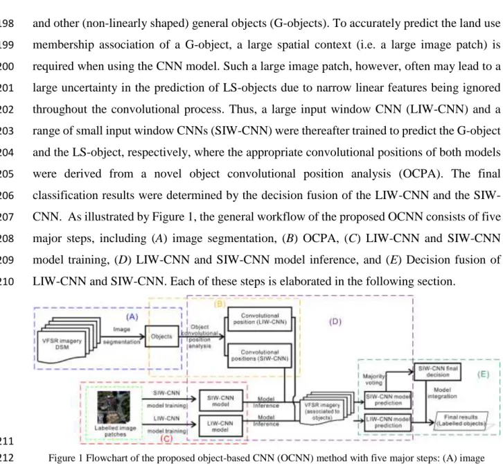
CNN. As illustrated by Figure 1, the general workflow of the proposed OCNN consists of five
207
major steps, including (A) image segmentation, (B) OCPA, (C) LIW-CNN and SIW-CNN
208
model training, (D) LIW-CNN and SIW-CNN model inference, and (E) Decision fusion of
209
LIW-CNN and SIW-CNN. Each of these steps is elaborated in the following section.
210
211
Figure 1 Flowchart of the proposed object-based CNN (OCNN) method with five major steps: (A) image
212
segmentation, (B) object convolutional position analysis (OCPA), (C) LIW-CNN and SIW-CNN model
213
training, (D) LIW-CNN and SIW-CNN model inference, and (E) fusion decision of LIW-CNN and SIW-CNN.
214
2.2.1 Image segmentation 215
The proposed method starts with an initial image segmentation to achieve an object-based
216
image representation. Mean-shift segmentation (Comaniciu and Meer, 2002), as a
217
nonparametric clustering approach, was used to partition the image into objects with
218
homogeneous spectral and spatial information. Four multispectral bands (Red, Green, Blue,
219
and Near Infrared) together with a digital surface model (DSM), useful for differentiating urban
220
objects with height information (Niemeyer et al., 2014), were incorporated as multiple input
221
data sources for the image segmentation (Figure 1(A)). A slight over-segmentation rather than
222
under-segmentation was produced to highlight the importance of spectral similarity, and all the
223
image objects were transformed into GIS vector polygons with distinctive geometric shapes.
8 2.2.2 Object convolutional position analysis (OCPA) 225
The object convolutional position analysis (OCPA) is employed based on the moment
226
bounding (MB) box of each object to identify the position of LIW-CNN and those of
SIW-227
CNNs. The MB box, proposed by Zhang and Atkinson, (2016), refers to the minimum
228
bounding rectangle built upon the moment orientation (the orientation of the major axis) of a
229
polygon (i.e. an object), derived from planar characteristics defined by mechanics (Zhang and
230
Atkinson, 2016; Zhang et al., 2006). The MB box theory is briefly described hereafter.
231
Suppose that (x, y) is a point within a planar polygon (S) (Figure 2), whose centroid isC(x,y).
232
The moment of inertia about the x-axis (Ixx ) and y-axis (Iyy), and the product of inertia (Ixy)
233
are expressed by Equations 2, 3 and 4, respectively.
234
y dA Ixx 2 (2) 235
x dA Iyy 2 (3) 236
xydA Ixy (4) 237Note, dA(= dxdy) refers to the differential area of point (x, y) (Timoshenko and Gere 1972).
238
239
Figure 2 A patch (S) with centroid C (x,y), dA is the differential area of point (x, y), Oxy is the geographic
240
coordinate system.
241
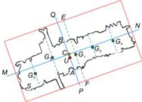
As illustrated by Figure 3, two orthogonal axes (MN and PQ), the major and minor axes, pass
242
through the centroid (C), with the minimum and maximum moment of inertia about the major
243
and minor axes, respectively. The moment orientation MB(i.e. the orientation of the major
244
axis) is calculated by Equations 5 and 6 (Timoshenko and Gere, 1972).
245 xx yy xy MB I I I 2 2 tan (5) 246
9 ) 2 ( tan 2 1 1 xx yy xy MB I I I (6) 247
The moment bounding (MB) box (the rectangle in red shown in Figure 3) that minimally
248
encloses the polygon, S, is then constructed by taking MBas the orientation of the long side
249
of the box, and EF is the perpendicular bisector of the MB box with respect to its long side.
250
The discrete forms of Equations 2-6 suitable for patch computation, are further deduced by
251
associating the value of a line integral to that of a double integral using Green’s theorem (see
252
Zhang et al. (2006) for theoretical details).
253
254
Figure 3 Moment bounding (MB) box and the CNN convolutional positions of a polygon S.
255
The CNN convolutional positions are determined by the minor axis (PQ) and the bisector of
256
the MB box (EF) to approximate the central region of the polygon (S). For the LIW-CNN, the
257
central point (the red point U) of the line segment (AB) intersected by PQ and polygon S is
258
assigned as the convolutional position. As for the SIW-CNN, a distance parameter (d) (a user
259
defined constant) is used to determine the number of SIW-CNN sampled along the polygon.
260
Given the length of a MB box as l, the number (n) of SIW-CNNs is derived as:
261 d d l n (7) 262
The convolutional positions of the SIW-CNN are assigned to the intersection between the
263
centre of the bisector (EF) as well as its parallel lines and the polygon S. The points (G1, G2, …,
264
G5) in Figure 3 illustrate the convolutional positions of SIW-CNN for the case of n = 5.
265
2.2.3 LIW-CNN and SIW-CNN model training 266
Both the LIW-CNN and SIW-CNN models are trained using image patches with labels as input
267
feature maps. The parameters and model structures of these two models are empirically tuned
268
as demonstrated in the Experimental Results and Analysis sections. Those trained CNN models
269
are used for model inference in the next stage.
10 2.2.4 LIW-CNN and SIW-CNN model inference 271
After the above steps, the trained LIW-CNN and SIW-CNN models, and the convolutional
272
position of LIW-CNN and those of SIW-CNN for each object are available. For a specific
273
object, its land use category can be predicted by the LIW-CNN at the derived convolutional
274
position within the VFSR imagery; at the same time, the predictions on the land use
275
membership associations of the object can also be obtained by employing SIW-CNN models
276
at the corresponding convolutional positions.Thus each object is predicted by both LIW-CNN
277
and SIW-CNN models.
278
2.2.5 Fusion decision of LIW-CNN and SIW-CNN 279
Given an object, the two LIW-CNN and SIW-CNN model predictions might be inconsistent
280
between each other, and the distinction might also occur within those of the SIW-CNN models.
281
Therefore, a simple majority voting strategy is applied to achieve the final decision of the
SIW-282
CNN model. A fusion decision between the LIW-CNN and the SIW-CNN is then conducted
283
to give priority to the SIW-CNN model for LS-objects, such as roads, railways etc.; otherwise,
284
the prediction of the LIW-CNN is chosen as the final result.
285
2.3 Accuracy assessment 286
Both pixel-based and object-based methods were adopted to comprehensively test the
287
classification performance using the testing sample set through five-fold cross validation. The
288
pixel-based approach was assessed based on the overall accuracy and Kappa coefficient as well
289
as per-class mapping accuracy computed from a confusion matrix. The object-based
290
assessment was based on geometry (Clinton et al., 2010; Li et al., 2015; Radoux and Bogaert,
291
2017). Specifically, suppose that a classified object Mi overlaps a set of reference objects Oij, 292
where j = 1, 2, ⋯r, r refers to the total number of reference objects overlapped by Mi. For each 293
pair of objects (Mi, Oij), a weight parameter deduced by the ratio between the area of a reference 294
object (area (Oij)) and the total area of reference objects
r
j 1area(Oij)was introduced to 295
calculate over-classification OC(Mi) and under-classification UC(Mi) error indices as: 296 1 1 area( ) area( ) ( ) ( (1 )), area( ) area( ) r i ij ij i r i ij j ij M O O OC M w w O O
(8) 297 1area( ) ( ) 1 area( ) r i ij j i i M O UC M M
(9) 29811
The total classification error (TCE) of Mi is designed to integrate the over-classification and 299
under-classification error as:
300 2 2 ( ) ( ) ( ) 2 i i i OC M UC M TCE M (10) 301
All three indices (i.e. OC, UC, and TCE) represent the average of all the classified objects for
302
each land use category in the classification map to formulate the final validation results.
303
3. Experimental Results and Analysis
304
3.1 Study area and data sources 305
In this research, two UK cities, Southampton (S1) and Manchester (S2), lying on the Southern
306
coast and in North West England, respectively, were chosen as our case study sites (Figure 4).
307
Both of the study areas are highly heterogeneous and distinctive from each other in land use
308
characteristics, and are thereby suitable for testing the generalization capability of the proposed
309
land use classification algorithm.
310
Aerial photos of S1 and S2 were captured using Vexcel UltraCam Xp digital aerial cameras on
311
22/07/2012 and 20/04/2016, respectively. The images have four multispectral bands (Red,
312
Green, Blue and Near Infrared) with a spatial resolution of 50 cm. The study sites were subset
313
into the city centres and their surrounding regions with spatial extents of 5802×4850 pixels for
314
S1 and 5875×4500 pixels for S2, respectively. Land use categories of the study areas were
315
defined according to the official land use classification system provided by the UK government
316
Department for Communities and Local Government (DCLG). Detailed descriptions of each
317
land use class and its corresponding sub-classes in S1 and S2 are listed in Tables 1 and 2,
318
respectively. 10 dominant land use classes were identified within S1, including high-density
319
residential, commercial, industrial, medium-density residential, highway, railway, park and
320
recreational area, parking lot, redeveloped area, and harbour and sea water. In S2, nine land
321
use categories were found, including residential, commercial, industrial, highway, railway,
322
park and recreational area, parking lot, redeveloped area, and canal.
12 324
Figure 4 The two study areas of urban scenes: S1 (Southampton) and S2 (Manchester).
325 326
Table 1. The land use classes in S1 (Southampton) and the corresponding sub-class components.
327
Land Use Class Train Test Sub-class Components
High-density residential 1026 684 Residential houses, terraces, a small coverage of green space Medium-density residential 984 656 Residential flats with a large green space and parking lots
Commercial 972 648 Commercial services with complex buildings, and parking lots
Industrial 986 657 Marine transportation, car factories
Highway 1054 703 Asphalt road, lane, cars
Railway 1008 672 Rail tracks, gravel, sometimes covered by trains
Parking lot 982 655 Asphalt road, parking line, cars
Park and recreational area 996 664 A large coverage of green space and vegetation, bare soil, lake Redeveloped area 1024 683 Bare soil, scattered vegetation, reconstructions
Harbour and sea water 1048 698 Sea shore, ship, sea water
328
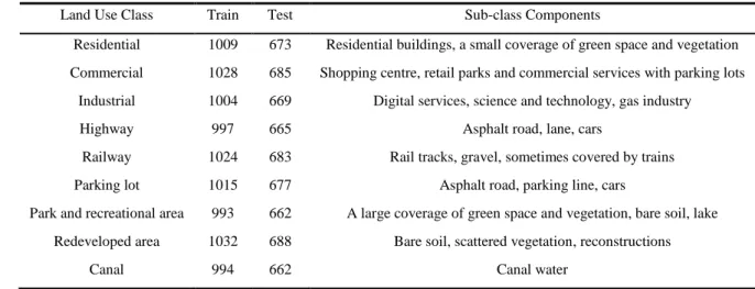
Table 2. The land use classes in S2 (Manchester) and the corresponding sub-class components.
329
Land Use Class Train Test Sub-class Components
Residential 1009 673 Residential buildings, a small coverage of green space and vegetation Commercial 1028 685 Shopping centre, retail parks and commercial services with parking lots
Industrial 1004 669 Digital services, science and technology, gas industry
Highway 997 665 Asphalt road, lane, cars
Railway 1024 683 Rail tracks, gravel, sometimes covered by trains
Parking lot 1015 677 Asphalt road, parking line, cars
Park and recreational area 993 662 A large coverage of green space and vegetation, bare soil, lake Redeveloped area 1032 688 Bare soil, scattered vegetation, reconstructions
Canal 994 662 Canal water
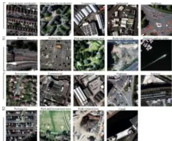
13 331
Figure 5 Representative exemplars (image patches) of each land use category at the two study sites (S1 and S2).
332
In addition to the above-mentioned aerial photographs, Digital Surface Models (DSM) of the
333
study sites with 50 cm spatial resolution were incorporated into the process of image
334
segmentation. Moreover, other data sources, including Google Maps, Microsoft Bing Maps,
335
and the MasterMap Topographic Layer (a highly detailed vector map from Ordnance Survey)
336
(Regnauld and Mackaness, 2006), were fully consulted and cross-referenced to gain a
337
comprehensive appreciation of the land cover and land use within the study sites.
338
Sample points were collected using a stratified random scheme from ground data provided by
339
local surveyors and photogrammetrists, and split into 60% training samples and 40% testing
340
samples for each class. The training sample size was guaranteed above an average of 1,000 per
341
class, which is sufficient for CNN networks, as recommended by Chen et al., (2016a). In S1, a
342
total of 10,080 training samples and 6,720 testing samples were obtained, and each category’s
343
sample size together with its sub-class components are listed in Table 1. In S2, 9,096 training
344
samples and 6,064 testing samples were acquired (see Table 2 for the detailed sample size per
345
class and the corresponding sub-classes). Figure 5 demonstrates typical examples of the land
346
use categories: note that they are highly heterogeneous and spectrally overlapping. Field
347
survey was conducted throughout the study areas in July 2016 to further check the validity and
348
precision of the selected samples.
349
3.2 Model structure and parameter settings 350
The proposed method was implemented based on vector objects extracted by means of image
351
segmentation. The objects were further classified through object-based CNN networks
352
(OCNN). Detailed parameters and model structures optimised by S1 and directly generalised
353
in S2 were clarified as follows.
14 3.2.1 Segmentation parameter settings
355
The initial mean-shift segmentation algorithm was implemented using the Orfeo Toolbox
356
open-source software. Two spatial and spectral bandwidth parameters, namely the spatial
357
radius and the range (spectral) radius, were optimized as 15.5 and 20 through cross-validation
358
coupled with a small amount of trial-and-error. In addition, the minimum region size (the scale
359
parameter) was chosen as 80 to produce a small amount of over-segmentation and, thereby,
360
mitigate salt and pepper effects simultaneously.
361
3.2.2 LIW-CNN and SIW-CNN model structures and parameters 362
Within the two study sites, the highway, railway in S1 and the highway, railway, and canal in
363
S2 belong to linearly shaped objects (LS-objects) in consideration of the elongated geometric
364
characteristics (e.g. Figure 6(B), (C)), while all the other objects belong to general objects
(G-365
objects) (e.g. Figure 6(A)). The LIW-CNN with a large input window (Figure 6(A)), and
SIW-366
CNNs with small input windows (Figure 6(B), (C)) that are suitable for the prediction of
G-367
objects and LS-objects, respectively, were designed here. Note, the other type of CNN models
368
employed on each object, namely, the SIW-CNNs in Figure 6(A) and the LIW-CNN in both
369
Figure 6(B) and 6(C) were not presented in the figure to gain a better visual effect. The model
370
structures and parameters of LIW-CNN and SIW-CNN are illustrated by Figure 7(a) and 7(b)
371
and are detailed hereafter.
372
373
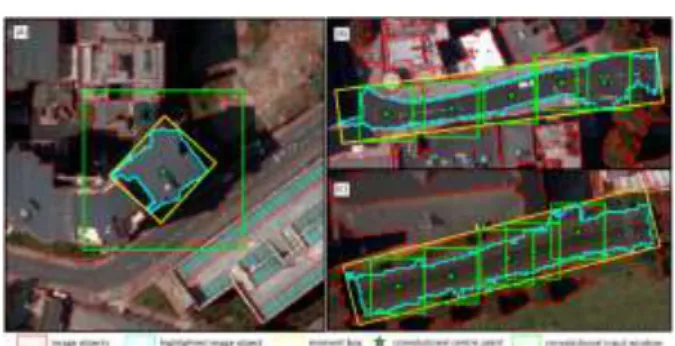
Figure 6 An illustration of object convolutional position analysis with the moment box (yellow rectangle), the
374
convolutional centre point (green star), and the convolutional input window (green rectangle), as well as the
375
highlighted image object (in cyan). All the other segmented objects are demonstrated as red polygons. (A)
376
demonstrates the large input window for a general object, and (B), (C) illustrate the small input windows for
377
linearly shaped objects (highway and railway, respectively, in these exemplars).
378
15
Figure 7 The model architectures and structures of the large input window CNN (LIW-CNN) with 128×128
380
input window size and eight-layer depth and small input window CNN (SIW-CNN) with 48×48 input window
381
size and six-layer depth.
382
The model structure of the LIW-CNN was designed similar to the AlexNet (Krizhevsky et al.,
383
2012) with eight layers (Figure 7(a)) using a large input window size (128×128), but with small
384
convolutional filters (3×3) for the majority of layers except for the first one (which was 5×5).
385
The input window size was determined through cross-validation on a range of window sizes,
386
including {48×48, 64×64, 80×80, 96×96, 112×112, 128×128, 144×144, 160×160} to
387
sufficiently cover the contextual information of general objects relevant to land use semantics.
388
The number of filters was tuned to 64 to extract deep convolutional features effectively at each
389
level. The CNN network involved alternating convolutional (conv) and pooling layers (pool)
390
as shown in Figure 7(a), where the maximum pooling within a 2×2 window was used to
391
generalize the feature and keep the parameters tractable.
392
The SIW-CNN (Figure 7(b)) with a small input window size (48×48) and six-layer depth is a
393
simplified structure with similar parameters to the LIW-CNN network, except for the number
394
of convolutional filters at each layer, which was reduced to 32 in order to avoid over-fitting the
395
model. The input window size was cross-validated on linear objects with a range of small
396
window sizes, including {24×24, 32×32, 40×40, 48×48, 56×56, 64×64, 72×72}, and 48×48
397
was found to be optimal to capture the contextual information about land use for linear objects.
398
All the other parameters for both CNN networks were optimized empirically based on standard
399
computer vision. For example, the number of neurons for the fully connected layers was set as
400
24, and the output labels were predicted through softmax estimation with the same number of
401
land use categories. The learning rate and the epoch were set as 0.01 and 600 to learn the deep
402
features through backpropagation.
403
3.2.3 OCNN parameter settings 404
In the proposed OCNN method, the LIW-CNN and the SIW-CNN networks were integrated to
405
predict the land use classes of general objects and linearly shaped objects at the model inference
406
phase. Based on object convolutional position analysis (OCPA), the LIW-CNN with a 128×128
407
input window (denoted as OCNN128) was employed only once per object, and the SIW-CNNs
408
with a 48×48 input window (denoted as OCNN48*, the 48* here represents multiple image
409
patches sized 48×48) were used at multiple positions to predict the land use label of an object
410
through majority voting (see section 2.2.2 for theoretical details). The parallel distance
16
parameter d in OCPA that controls the convolutional locations and the number of small window
412
size CNNs, was estimated by the length distribution of the moment box together with a
trial-413
and-error procedure in a wide search space (0.5 m – 20 m) with a step of 0.5 m. The d was
414
optimized as 5 m for the objects with moment box length (l) larger than or equal to 20 m, and
415
was estimated by l/4 for those objects with l less than 20 m (i.e. the minimum number of small
416
window size CNNs was 3) to perform a statistical majority voting. The proposed method
417
(OCNN128+48*) integrates both OCNN128 and OCNN48*, which is suitable for the prediction of
418
urban land use semantics for any shaped objects.
419
3.2.4 Other benchmark methods and their parameters 420
To evaluate the classification performance of the proposed method, three existing benchmark
421
methods (i.e. Markov Random Field (MRF), object-based image analysis with support vector
422
machine (OBIA-SVM), and the pixel-wise CNN) that each incorporate spatial context were
423
compared comprehensively, as follows:
424
MRF: The Markov Random Field, a spatial contextual classifier, was used as a benchmark
425
comparator. The MRF was constructed by the conditional probability formulated by a support
426
vector machine (SVM) at pixel level, which was parameterized through grid search with a
5-427
fold cross-validation. The spatial context was incorporated by a fixed size of neighbourhood
428
window (7×7) and a parameter γ that controls the smoothness level, set as 0.7, to achieve an
429
appropriate level of smoothness in the MRF. The simulated annealing optimization approach
430
with a Gibbs sampler (Berthod et al., 1996) was employed in the MRF to maximize the
431
posterior probability through iteration.
432
OBIA-SVM: The multi-resolution segmentation was implemented initially to segment objects
433
through the image. A range of features was further extracted from these objects, including
434
spectral features (mean and standard deviation), texture (grey-level co-occurrence matrix) and
435
geometry (e.g. perimeter-area ratio, shape index). In addition, the contextual pairwise similarity
436
that measures the degree of similarity between an image object and its neighbouring objects
437
was deduced to account for the spatial context. All these hand-coded features were fed into a
438
parameterized SVM for object-based classification.
439
Pixel-wise CNN: The standard pixel-wise CNN was trained to predict all pixels within the
440
images using densely overlapping image patches. The most important parameters that influence
441
directly the classification performance of the pixel-wise CNN are the input image patch size
442
and the number of layers (depth). Following the discussion by Längkvist et al., (2016), the
17
input image size was chosen from {28×28, 32×32, 36×36, 40×40, 44×44, 48×48, 52×52 and
444
56×56} to evaluate the influence of contextual area on classification performance. The optimal
445
input image patch size for the pixel-wise CNN was found to be 48×48 to leverage the training
446
sample size and the computational resources (e.g. GPU memory). The depth configuration of
447
the CNN network plays a key role in classification accuracy because the quality of the learnt
448
features is highly influenced by the level of abstraction and representation. As suggested by
449
Chen et al., (2016a), the number of CNN layers was chosen as six to balance the network
450
complexity and robustness. Other CNN parameters were tuned empirically through
cross-451
validation. For example, the filter size was set to 3×3 for the convolutional layer with a stride
452
of 1, and the number of filters was set to 24 to extract multiple convolutional features at each
453
level. The learning rate was set as 0.01 and the number of epochs was chosen as 600 to fully
454
learn the features through backpropagation.
455
3.3 Classification results and analysis 456
The classification performance of the proposed OCNN128+48* method using the
above-457
mentioned parameters was investigated on both S1 (experiment 1) and S2 (experiment 2). The
458
proposed method was compared with OCNN128 and OCNN48* as well as the benchmark MRF,
459
OBIA-SVM and the pixel-wise CNN. Visual inspection and quantitative accuracy assessment,
460
including pixel-based overall accuracy (OA), Kappa coefficient (κ) and the per-class mapping
461
accuracy as well as object-based accuracy assessment, were adopted to evaluate the
462
classification results hereafter.
463
Experiment 1: A desirable classification result was obtained in S1 by using the proposed
464
OCNN128+48*. To provide a useful visualization, three subsets of S1 classified by different
465
approaches were presented in Figure 8, with the correct or incorrect classification results
466
marked in yellow or red circles, respectively. In general, the proposed method achieved the
467
smoothest visual results with precise boundary information compared with other benchmark
468
methods. Most importantly, the semantic contents of complex urban land uses (e.g. commercial,
469
industrial etc.) were effectively characterized, and the linearly shaped features including
470
highway and railway were identified with high geometric fidelity. As shown by Figure 8(a)
471
and 8(c), the highway (a linear feature) was misclassified as a parking lot (red circles) by
472
OCNN128, whereas the highway feature was accurately identified by the OCNN48* (yellow
473
circles). However, OCNN48* was inferior to OCNN128 when identifying general objects, as
474
demonstrated by Figure 8(b). Fortunately, these complementary behaviours of the two
18
modules were captured by the proposed OCNN128+48*, which was able to label the highway
476
accurately (yellow circles in Figure 8(b)). The pixel-wise CNN demonstrated some capacity
477
for extracting semantic functions for complex objects; for example, the commercial area in
478
Figure 8(b) was correctly distinguished (yellow circle). However, classification errors along
479
the edges or boundaries between objects were found. For example, the edges of the highway
480
were misclassified as high-density residential as shown by Figure 8(a). For the OBIA-SVM,
481
the simple land uses with less within-object variation (e.g. highway) were more accurately
482
classified (yellow circle in Figure 8(a) and 8(c)), whereas, those highly complex land uses with
483
great within-object variation (e.g. commercial, industrial etc.) were more likely to be
484
misclassified (red circle in Figure 8(b)). In addition, the OBIA-SVM could also discover some
485
sub-objects (e.g. balcony on the residential house) through the information context. The results
486
of the MRF, in contrast to the other object-based approaches, were the least smooth even
487
though local neighbourhood information was used. Nevertheless, there were still some benefits
488
of the MRF: spectrally distinctive land uses, such as highway, park and recreational area, were
489
classified with a relatively high accuracy.
490
491
Figure 8 Three typical image subsets (a, b and c) in study site S1 with their classification results. Columns from
492
left to right represent the original images (R G B bands only), and the MRF, OBIA-SVM, Pixel-wise CNN,
493
OCNN48*, OCNN128, and the proposed OCNN128+48* results. The red and yellow circles denote incorrect and 494
correct classification, respectively.
495 496
The effectiveness of the OCNN128+48* was also demonstrated by quantitative classification
497
accuracy assessment. As shown in Table 2, the OCNN128+48* achieved the largest overall
498
accuracy of 89.52% with a Kappa coefficient (κ) of 0.88, consistently larger than its
sub-499
module OCNN128 (87.31% OA and κ of 0.86) and the OCNN48* (OA of 84.23% and κ of 0.82),
500
respectively. The accuracy increase was much more dramatic in comparison with other
19
benchmark methods, including the pixel-wise CNN (81.62% OA and κ of 0.80), the
OBIA-502
SVM (79.54% OA and κ of 0.78), as well as the MRF (OA of 78.67% and κ of 0.76). The
503
superiority of the proposed OCNN128+48* was further demonstrated by the per-class mapping
504
accuracy (Table 3). From the table, it can be seen that the accuracies of highway and railway
505
were increased significantly by 5.34% and 4.64% respectively, compared with the OCNN128.
506
This was followed by a moderate increase of 3.24% for the parking lot class. Other land use
507
classes (e.g. commercial, industrial, etc.) were slightly increased in terms of classification
508
accuracy (less than 1.5%) without statistical significance in comparison with OCNN128. When
509
comparing with the OCNN48*, the accuracy increase of the proposed OCNN128+48* was
510
remarkable for the majority of general object classes, with increases of up to 6.06%, 6.51%,
511
4.98%, 4.7% and 4.68%, for the classes of commercial, industrial, redeveloped area, park and
512
recreational area, and high-density residential, respectively; whereas the accuracies of the
513
medium-density residential and the parking lot increased moderately, by 3.31% and 3.81%,
514
respectively. For linearly shaped objects, however, the OCNN128+48* was not substantially
515
superior to the OCNN48*, with just a slight accuracy increase of 1.52% for highway and 2.41%
516
for railway, respectively. For general objects with complex semantic functions, including
517
commercial, industrial, redeveloped area, park and recreational area, and high-density
518
residential, the increase in accuracy of the OCNN128+48* was much more significant, by up to
519
6.06%, 6.51%, 4.98%, 4.7% and 4.68%, respectively.
520
In terms of the pixel-wise CNN, effectiveness was observed for certain complex objects (e.g.
521
the accuracy for the industrial land use was up to 80.23%). However, the simple and
522
geometrically distinctive land use classes were not accurately mapped, with the largest
523
accuracy difference up to 6.57% for the class highway compared with the OCNN128+48*. By
524
contrast, the OBIA-SVM demonstrated some advantages on simple land use classes (e.g. the
525
accuracy of railway up to 90.65%), but it failed to accurately identify more complex general
526
objects (e.g. an accuracy as low as 71.87% for commercial land use). The MRF presented the
527
smallest classification accuracy for most land use classes, especially the complex general land
528
uses (e.g. 12.37% accuracy lower than the OCNN128+48* for commercial land use).
529 530
Table 3. Classification accuracy comparison amongst MRF, OBIA-SVM, Pixel-wise CNN, OCNN48*, OCNN128, 531
and the proposed OCNN128+48* method for Southampton using the per-class mapping accuracy, overall accuracy 532
(OA) and Kappa coefficient (κ). The bold font highlights the greatest classification accuracy per row.
533
Class MRF OBIA-SVM Pixel-wise CNN OCNN48* OCNN128 OCNN128+48*
20
highway 77.23 78.04 76.12 78.17 74.35 79.69
industrial 67.28 69.01 71.23 78.24 83.87 84.75
high-density residential 81.52 80.59 80.05 81.75 85.35 86.43
medium-density residential 82.74 84.42 85.27 87.28 90.34 90.59
park and recreational area 91.05 93.14 92.34 92.59 96.41 97.09
parking lot 80.09 83.17 84.76 86.02 85.59 88.83
railway 88.07 90.65 86.57 89.51 87.28 91.92
redeveloped area 89.13 90.02 89.26 89.71 94.57 94.69
harbour and sea water 97.39 98.43 98.54 98.62 98.75 98.95
Overall Accuracy (OA) 78.67% 79.54% 81.62% 84.23% 87.31% 89.52%
Kappa Coefficient (κ) 0.76 0.78 0.8 0.82 0.86 0.88
534
An object-based accuracy assessment was implemented in S1 to validate the classification
535
performance in terms of over-classification (OC), under-classification (UC), and total
536
classification error (TCE). Three typical methods, including OBIA-SVM (denoted as OBIA),
537
pixel-wise CNN (denoted as CNN), and the proposed OCNN128+48* method (denoted as OCNN),
538
were evaluated, with accuracy comparisons of each land use class listed in Table 4. Clearly,
539
the proposed OCNN method produced the smallest OC, UC, and TCE errors, respectively
540
(highlighted by bold font), constantly smaller than those of the CNN and OBIA. Generally, the
541
UC errors are smaller than OC errors, demonstrating that a slight over-segmentation was
542
produced. Specifically, the OCNN demonstrates excellent object-level classification, with the
543
majority of classes less than 0.2 in TCE. Those complex land use classes, including commercial
544
and industrial, can be segmented precisely and classified with small TCE of 0.22 and 0.20, less
545
than those of CNN (0.29 and 0.27) and OBIA (0.39 and 0.38). The parking lot objects with
546
complex land use patterns, were also recognised accurately with high fidelity (OC of 0.22, UC
547
of 0.13, and TCE of 0.17), less than CNN (0.28, 0.17, and 0.22) as well as OBIA (0.41, 0.32,
548
and 0.37). For those LS-objects, the OCNN achieved promising accuracy in comparison with
549
the other two benchmarks. For example, the TCEs of highway and railway produced by the
550
OCNN were 0.17 and 0.09, smaller than those of the CNN (0.25 and 0.22) and OBIA (0.20 and
551
0.18). All the other land use categories demonstrate increased segmentation accuracy. For
552
instance, the TCE of park and recreational area was 0.18 with the OCNN, less than for the CNN
553
of 0.24 and OBIA of 0.32.
554 555
Table 4 Object-based accuracy assessment among OBIA-SVM (OBIA), Pixel-wise CNN (CNN), and the
556
proposed OGC-CNN128+48* method (OCNN) for Southampton using error indices of OC, UC, and TCE. The bold 557
font highlights the smallest classification error of a specific index per row.
558
Class OC UC TCE
21 commercial 0.45 0.33 0.26 0.34 0.26 0.18 0.39 0.29 0.22 highway 0.23 0.29 0.19 0.17 0.21 0.16 0.20 0.25 0.17 industrial 0.42 0.31 0.23 0.36 0.24 0.17 0.38 0.27 0.20 high-density residential 0.34 0.28 0.14 0.26 0.19 0.08 0.30 0.23 0.11 medium-density residential 0.29 0.21 0.16 0.21 0.14 0.09 0.25 0.17 0.12
park and recreational area 0.36 0.29 0.24 0.28 0.19 0.12 0.30 0.24 0.18
parking lot 0.41 0.28 0.22 0.32 0.17 0.13 0.37 0.22 0.17
railway 0.25 0.27 0.12 0.11 0.18 0.06 0.19 0.21 0.09
redeveloped area 0.37 0.32 0.21 0.29 0.25 0.13 0.33 0.28 0.17
harbour and sea water 0.18 0.19 0.14 0.07 0.11 0.06 0.12 0.15 0.09
559
Experiment 2: The most accurate classification performance was also achieved in S2 by the
560
proposed method, as illustrated by the quantitative accuracy results in Table 5. From the table,
561
it can be seen that OCNN128+48* obtained the greatest overall accuracy (OA) of 90.87% with a
562
Kappa coefficient (κ) of 0.88, significantly larger than the OCNN128 (OA of 88.74% and κ of
563
0.86), the OCNN48* (OA of 85.06% with κ of 0.83), the Pixel-wise CNN (OA of 82.39% and
564
κ of 0.81), the OBIA-SVM (OA of 80.37% with κ of 0.79), and the MRF (OA of 78.52% with
565
κ of 0.76). The effectiveness of the OCNN128+48* was also demonstrated by the per-class
566
mapping accuracy. Compared with the OCNN128, the classes formed by linearly shaped objects,
567
including the highway, railway and canal, had significantly increased accuracies of up to 5.36%,
568
3.06% and 3.48%, respectively (Table 5). Such increases can also be noticed in Figure 9 (a
569
subset of S2), where the misclassifications of railway and highway shown in Figure 9(g) were
570
rectified in Figure 9(h) classified by the OCNN128+48*. At the same time, the parking lot land
571
use class was moderately increased by 2.28%. Whereas, other land use classes had slightly
572
increases in accuracy of less than 1% on average. In contrast, the OCNN128+48* led to no
573
significant increases over the OCNN48* for the linear object classes, with accuracy increases
574
for highway, railway and canal of 1.8%, 0.42% and 1.22%, respectively. For the general classes,
575
especially the complex land uses (e.g. commercial, industrial etc.), remarkable accuracy
576
increases were achieved with an average up to 6.75%. Figure 9(f) (classified by OCNN48*) also
577
showed the confusion between the commercial and industrial land use classes, which was
578
revised in Figure 9(h). With respect to the benchmark comparators, the accuracy increase of
579
OCNN128+48* was much more obvious for most of the land use classes, with the largest accuracy
580
increase up to 12.39% for parking lot, 11.21% for industrial, and 8.56% for commercial,
581
compared with the MRF, OBIA-SVM and Pixel-wise CNN, respectively. The undesirable
582
visual effects and misclassifications can also be seen in Figure 9(c-e), which were corrected in
583
Figure 9(h).
22 585
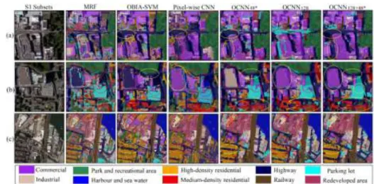
Figure 9 Classification results in study site S2, with (a) an image subset (R G B bands only), (b) the ground
586
reference, (c) MRF classification, (d) OBIA-SVM classification, (e) Pixel-wise CNN classification, (f) OCNN48* 587
classification, (g) OCNN128 classification, and (h) OCNN128+48* classification. 588
589
Table 5 Classification accuracy comparison amongst MRF, OBIA-SVM, Pixel-wise CNN, OCNN48*, OCNN128, 590
and the proposed OCNN128+48* method for Manchester, using the per-class mapping accuracy, overall accuracy 591
(OA) and Kappa coefficient (κ). The bold font highlights the greatest classification accuracy per row.
592
Class MRF OBIA-SVM Pixel-wise CNN OCNN48* OCNN128 OCNN128+48*
commercial 71.11 72.47 74.16 76. 27 82.43 82.72 highway 80.43 79.26 80.59 82.57 79.01 84.37 industrial 73.52 72.05 74.84 76.22 82.19 83.26 residential 78.41 80.45 80.56 83.09 84.75 84.99 parking lot 79.63 82.06 84.37 87.86 89.74 92.02 railway 85.94 88.14 88.32 91.06 88.42 91.48
park and recreational area 88.42 89.54 90.76 91.34 94.38 94.59
redeveloped area 82.07 84.15 87.04 88.83 93.16 93.75
canal 90.02 92.28 94.18 97.52 95.26 98.74
Overall Accuracy (OA) 78.52% 80.37% 82.39% 85.06% 88.74% 90.87%
Kappa Coefficient (κ) 0.76 0.79 0.81 0.83 0.86 0.88
593
Similar to S1, the object-based accuracy assessment was conducted in S2 to investigate the
594
over-, under-, and total classification errors of each class using the OCNN, CNN and OBIA
595
methods (Table 6). The error indices in S2 (Table 6) present a similar trend with those in S1
596
(Table 4), although the geometric errors for S2 are smaller than for S1 due to the relatively
597
regular land use structures and configurations in Manchester city centre. The proposed OCNN
598
yielded the greatest classification accuracy with the smallest error indices (highlighted by bold
599
font), smaller than those of the CNN and OBIA. The OCNN accurately differentiated the
600
complex land use classes, with a TCE of 0.20, 0.17, and 0.15 for the classes of commercial,
601
industrial and parking lot, respectively (Table 6), significantly smaller than for the CNN (0.27,
602
0.26, and 0.24), and OBIA (0.37, 0.35, and 0.32). Those linearly shaped objects, including
23
highway, railway, and canal, were precisely characterised by the OCNN method, with a TCE
604
of 0.16, 0.09, and 0.08, significantly smaller than for the CNN (0.22, 0.21, and 0.14) and OBIA
605
(0.18, 0.19, and 0.12). The residential land use was also clearly improved with a very small
606
TCE of 0.10, smaller than for the CNN (0.22) and OBIA (0.26). Other land use classes, such
607
as the park and recreational area and the redeveloped area, were also better distinguished by
608
the OCNN (0.16 and 0.15 in terms of TCE), smaller than for the CNN (0.21 and 0.25) and
609
OBIA (0.28 and 0.30).
610
Table 6 Object-based accuracy assessment among OBIA-SVM (OBIA), Pixel-wise CNN (CNN), and the
611
proposed OGC-CNN128+48* method (OCNN) for Manchester using error indices of OC, UC, and TCE. The bold 612
font highlights the lowest classification error of a specific index per row.
613
Class OC UC TCE
OBIA CNN OCNN OBIA CNN OCNN OBIA CNN OCNN
commercial 0.41 0.32 0.24 0.32 0.23 0.16 0.37 0.27 0.20 highway 0.22 0.27 0.18 0.15 0.19 0.15 0.18 0.23 0.16 industrial 0.39 0.31 0.20 0.31 0.22 0.14 0.35 0.26 0.17 residential 0.30 0.24 0.12 0.22 0.20 0.09 0.26 0.22 0.10 parking lot 0.37 0.26 0.19 0.28 0.22 0.12 0.32 0.24 0.15 railway 0.22 0.25 0.10 0.14 0.19 0.07 0.18 0.22 0.09
park and recreational area 0.31 0.25 0.21 0.26 0.17 0.10 0.28 0.21 0.16
redeveloped area 0.34 0.29 0.18 0.26 0.22 0.12 0.30 0.25 0.15
canal 0.16 0.17 0.12 0.08 0.12 0.05 0.12 0.14 0.08
614
A sensitivity analysis was conducted to further investigate the effect of different input window
615
sizes on the overall accuracy of urban land use classification (see Figure 10). The window sizes
616
varied from 16×16 to 144×144 with a step size of 16. From Figure 10, it can be seen that both
617
S1 and S2 demonstrated similar trends for the proposed OCNN and the pixel-wise CNN (CNN).
618
With window sizes smaller than 48×48 (i.e. relatively small windows), the classification
619
accuracy of OCNN is lower than that of CNN, but the accuracy difference decreases with an
620
increase of window size. Once the window size is larger than 48×48 (i.e. relatively large
621
windows), the overall accuracy of the OCNN increases steadily until the window is as large as
622
128×128 (up to around 90%), and outperforms the CNN which has a generally decreasing trend
623
in both study sites. However, an even larger window size (e.g. 144×144) in OCNN could result
624
in over-smooth results, thus reducing the classification accuracy.
24 626
Figure 10 The influence of CNN window size on the overall accuracy of pixel-wise CNN and the proposed
627
OCNN method for both study sites S1 and S2.
628 629
3.4 Computational efficiency 630
The computational efficiency of the proposed method was evaluated and compared with the
631
other methods listed in Table 7. The classification experiments were implemented using
632
Keras/Tensorflow under a Python environment with a laptop of NVIDIA 940M GPU and 12.0
633
GB memory. As shown in Table 7, the training time of the Pixel-wise CNN, OCNN48*,
634
OCNN128 and the proposed OCNN128+48* were similar in both experiments, with an average
635
time of 4.27 h, 4.36 h, 4.74 h, and 4.78 h, respectively. The prediction time for the Pixel-wise
636
CNN was the longest compared with other OCNN-based approaches with 321.07 h on average,
637
about 100 times longer than those of the OCNN-based approaches. Among the three OCNN
638
methods, the OCNN128 and the OCNN128+48* were similar in computational efficiency with
639
average of 2.81 h and 2.9 h, respectively, longer than that of the OCNN48* (1.78 h on average)
640
for the two experiments. The benchmark methods, the MRF and OBIA-SVM, spent much less
641
time on the training and prediction phases than the CNN-based methods, with an average of
642
1.4 h and 1.2 h for the two experiments, about 20 times and 3 times less than the pixel-wise
643
CNN and the OCNN-based approaches, respectively.
644
Table 7. Comparison of computational times amongst MRF, OBIA-SVM, Pixel-wise CNN, OCNN48*, OCNN128, 645
and the proposed OCNN128+48* approach in S1 and S2. 646 Study area No. of object Mean Area (m2) Computation time (h) MRF OBIA-SVM Pixel-wise
CNN OCNN48* OCNN128 OCNN128+48*
Train S1 6328 25.37 1.42 0.58 4.45 4.45 4.88 4.92 S2 6145 25.92 1.37 0.44 4.08 4.27 4.59 4.64 Predict S1 61 921 26.61 1.52 1.76 326.78 1.82 2.83 2.94 S2 58 408 25.75 1.33 1.55 315.36 1.74 2.78 2.86 647 648 649