School system evaluation by value-added analysis under endogeneity

(1)

2010/46

■

School system evaluation by

value-added analysis under endogeneity

Jorge Manzi, Ernesto San Martin

and Sébastien Van Bellegem

Center for Operations Research

and Econometrics

Voie du Roman Pays, 34

B-1348 Louvain-la-Neuve

Belgium

http://www.uclouvain.be/core

(2)

CORE DISCUSSION PAPER 2010/46

School system evaluation by value-added analysis under endogeneity

Jorge MANZI 1_{, Ernesto SAN MARTIN}2

and Sébastien VAN BELLEGEM 3

July 2010

Abstract

Value-added analysis is a common tool in analysing school performances. In this paper, we analyse the SIMCE panel data which provides individual scores of about 200,000 students in Chile, and whose aim is to rank schools according to their educational achievement. Based on the data collection procedure and on empirical evidences, we argue that the exogeneity of some covariates is questionable. This means that a nonvanishing correlation appears between the school-specific effect and some covariates. We show the impact of this phenomenon on the calculation of the value-added and on the ranking, and provide an estimation method that is based on instrumental variables in order to correct the bias of endogeneity. Revisiting the definition of the value-added, we propose a new calculation robust to endogeneity that we illustrate on the SIMCE data.

Keywords: value-added, school effectiveness, multilevel model, endogeneity, instrumental variables.

JEL Classification: Primary C33, secondary C51, I21

1_{Measurement Center MIDE UC (Pontificia Universidad Cat}_ó_{lica de Chile, Chile).}

2_{Measurement Center MIDE UC & Dep. Of Statistics (Pontificia Universidad Cat}_ó_{lica de Chile, Chile).}

3 _{Toulouse School of Economics, France;}

Université catholique de Louvain, CORE, B-1348 Louvain-la-Neuve, Belgium. E-mail: [email protected]

We thank Jorge González, Jean Hindriks, Daniel Koretz, Michel Mouchart, Sally Thomas and Marijn Vershelde for helpful discussions. This paper was presented at the International Meeting on School Progress and Value-added Models organized by the Measurement Center MIDE UC, May 2010, Santiago, Chile. This work was supported by the “Agence National de le Recherche” under contract ANR-09-JCJC-0124-01 and the CORFO INNOVA Grant No. 07CN13IEM-91 Development of standardized tests and of a value-added methodology to assess progress of learning in Mathematics and Language students, second cycle of primary school. The authors are grateful to the SIMCE Office of the Chilean Ministry of Education for providing access to the database. All opinions and conclusions expressed in this paper are those of the authors and not of the Ministry of Education. This paper presents research results of the Belgian Program on Interuniversity Poles of Attraction initiated by the Belgian State, Prime Minister's Office, Science Policy Programming. The scientific responsibility is assumed by the authors.

(3)

1 Introduction

A typical way to measure the school performance is to compare the progress that students make between two or more test occasions. Among the numerous measurement methods, the “value-added analysis” has often been considered in empirical studies (see e.g. OECD (2008) and the references therein). The value-added analysis aims at measuring the gain (or the loss) of beeing in a given school with respect to an average school. This average school is defined as the average performance of the schools that are found in the data set, and there-fore the value-added provides a data-driven measure of school effectiveness. Another aspect of the value-added analysis is that it usualy controls for a set of variables such as individ-ual characteristics (e.g. students gender or socio-economic level) or school/environmental characteristics. Moreover, the previous attained score of the students is always considered as a control variable.

Measuring the value-added requires an appropriate model for the test score. Due to the hierarchical structure found in educational data sets, the multilevel generalized linear model is used routinely in this analysis. In the statistical parlance, the value-added in this model is calculated as the predictor of the random school-effect of the multilevel regression (Raudenbush and Willms, 1995; Tekweet al., 2004).

The recent literature however has shown that systematic bias problems occur in the inference for the multilevel model on educational data. A typical source of bias is due to omitted variables (Kim and Frees, 2006; Lockwood and McCaffrey, 2007). The reason may be explained as follows. We have recalled that the multilevel regression model used in the value-added analysis contains the prior attainment score as a regressor. Suppose that a variable is omitted in this model and this variable is correlated with both the actual test score and the prior test score. Because the variable is omitted, it is therefore included in the error term of the multilevel model. Therefore, the error of the model is not uncorrelated with the prior attainment score. This correlation is a source of bias in the standard estimation for regression model, and is sometimes called an endogeneity bias (Halaby, 2004; Steele, Vignoles and Jenkins, 2007).

The last argument will be extensively described and discussed in this paper. It has an important impact on the inference for multilevel models because it is not obvious to understand which variable is omitted or, if so, it is not always easy to measure this omitted variable. For instance, the school effect is by definition unobserved and is influential on both the previous attainment score and the actual score, provided that the student has not switched schools between the two tests. In more technical terms, there is a non vanishing correlation between the random school-effect and the prior attaintment score as soon as the student has already been “treated” by its school at the time of the first test occasion. This shows why the endogeneity bias is systematic when there is little movement of students between test occasions.

The literature contains some methods of estimation to circumvent the endogeneity bias in multilevel models. Two major contributions are Ebbes, B¨ockenholt and Wedel (2004) and Kim and Frees (2007), and we also cite the recent work of Grilli and Rampichini (2009) in the context of general measurement errors. The present paper aims to study the impact of the endogeneity on the measure of the value-added. We show that, in the presence of

(4)

endogeneity, an additive correcting term must be applied on the usual calculation of the value-added indicator of a school. We provide the exact form of the correction term and show how to calculate it from data.

Our methodology is motivated and illustrated by the study of the Chilean school per-formance. A rich dataset is used in which the score in mathematics and other covariates of 163,286 students from 1,886 schools were measured in 2004 and 2006. A description of the Chilean educational system and of the research on school effectiveness in that country is to be found in Section 2 below. In Section 3, the dataset is described. Section 4 starts with a structural definition of the value-added and shows the result of a value-added analysis under standard assumptions (e.g. under exogeneity of all covariates). In Section 4.3, we argue that the endogeneity of some covariates is not avoidable and we describe the impact of this endogeneity on the value-added. The calculated value-added may be used in order to rank schools according to their performance. We show what is the impact of the endogene-ity on the school ranking. In Section 4.4, we demonstrate how the value-added has to be corrected, and we show the impact of this correction on the value-added of the 1,886 chilean schools. A formal definition of the multilevel model under endogeneity is also presented in the Appendix. The appendix describes the steps that are used in order to calculate the value-added under endogeneity.

2 Chilean Educational System and School Effectiveness

Re-search

2.1 The SIMCE test

One of the most important aspects in the development and achievements of a country is having a satisfactory educational system that is accessible to all, or the big majority, of its individuals. In Chile, it is widely acknowledged that the state of its educational system is a hindrance to its development. A key aspect that has been criticized is the poor quality of some school teachers with limited knowledge of the material that they need to teach. Another aspect is the inequality between public schools and private schools (see OECD (2007)). However during the last decades Chile has worked to improve the quality of its education leading to the generation of novel public policies to tackle a part of the problems. Some examples are the increase in the amount of time that students should spend at school, and a new law stating that it is mandatory that all students get education for the four years that correspond to secondary education. The Preferential Subsidy Law (passed by the Senate on May 4, 2009) is another example. Broadly speaking, this new law fixes conditions to evaluating students’ performance and, based on them, to classify schools into three types: charter school, emerging school, and recovery school. Economical and administrative support are provided to schools according to that classification.

With the aim of uncovering the possible causes of deficiency in the educational system, the Chilean government has been systematically gathering data since 1988 about students’ performance. This large scale data collection is known as the SIMCE test (SIMCE stands forSistema de Medici´on de Calidad de la Educaci´on). This policy is consistent with what

(5)

the Organization for Economic Co-operation and Development (OECD) has found to be the first step to unveil the problems in the educational system (OECD, 2008). Together with the national voucher system, a national evaluation of student performance was conceived that would provide parents with necessary information to make decisions about schools. In 1988, students in all Chilean schools begun to be tested with the SIMCE test, which was given in alternating years in 4th and 8th grade, and later in 1994, also in 10th grade. Since 2005, the SIMCE test was applied all the years to 4th grade. Until 1994, SIMCE results were delivered only in aggregates, they were given only to schools and Municipalities, and were not comparable for different years. Starting in 1995, the SIMCE results by schools begun being publicized through the media, with the aim of contributing to its original purpose of providing information for parents to make decisions about schools.

In 1998, SIMCE suffered several changes. First, an effort was made to tightly tie the SIMCE tests into the educational goals and contents specified in the new national curricula defined by the Chilean Ministry of Education. Together with this, the instruments were modified to include not only multiple choice questions, but also open questions devoted to test more complex skills such as critical thinking or written expression. The complemen-tary questionnaires for parents and school principals were also modified in order to collect better quality information at the individual level. In 2000, results of the SIMCE started to be published by group of schools having a comparable socioeconomic status, in order to facilitate comparisons between schools that educate similar students. With the aim to improve the quality of teaching, the government also asked to provide example of questions and solutios in the final report of the SIMCE test given to schools. For an example of a SIMCE report, see SIMCE (2009).

With regards to the instruments themselves, Item Response Theory methodology has been introduced in 2000, allowing comparisons across years, and making it possible to produce more accurate descriptions of different levels of performance, to measure with precision students with different skill levels, and to examine possible item bias. For details, see SIMCE (2008).

Taking into account the calendar of the SIMCE applications, it is possible for each stu-dent to obtain two measures of their educational performance. Most of these measurements will be taken every four years; for instance, students who were measured in 2005, were still measured in 2009 when they were in the 8th grade. In the study reported in this paper, we considered students who were measured in 2004 (when they were at the 8th grade) and in 2006 (when they were at the 10th grade).

2.2 The Chilean educational system

The Chilean education system has suffered several changes in the last three decades. In 1980, elements of privatization and decentralization were introduced through a massive voucher system by which private schools were allowed to receive a state subsidy proportional to the number of students attending classes, as long as they met certain requirements. At the same time, administration of public schools was shifted from the Ministry of Education to local authorities (Municipalities). Up to 1980, the Ministry of Education was in charge of financing public education, establishing educational contents and investing in infrastructure.

(6)

After the 1980’s reform, the Ministry retained authority over educational contents and goals, and it was responsible for supervising the functioning of schools receiving voucher monies, while infrastructure and hiring decisions were delegated to local school administrators, both public and private. As a consequence of the introduction of private operators into the system, a new group of schools was created – private-subsidized schools – and this increased the number of schools significantly in later years.

From 1990, a significant increase in public investment in education was registered. This increase in investment had a clear impact on education coverage. According to Bellei (2005), between 1990 and 2000 this raised coverage in primary education from 93% to 98% and from 74% to 85% in secondary education. However, increases in educational quality, as measured by standardized tests, were not evident. It is likely that the increases in education coverage in those years have actually lowered average test scores, as children who would otherwise have been outside the school system begin to enter school. In spite of this, test scores have not experienced a drop. For example, in 2003 there was a 20% increment over the previous year in the number of students taking the national SIMCE tests, but average SIMCE scores did not drop significantly.

In 1991, the “Estatuto Docente” was created, establishing regulations for teacher salaries and protecting them from being fired from the Municipal system, tending to make the system more rigid. Also in 1991, a number of improvement programs were put in place that targeted schools which cater to the most vulnerable students. In 1993 shared financing is introduced, which allowed private-subsidized and secondary public schools to charge parents a fee in addition to the state voucher, provide that this fee does not exceed a certain value. Primary public schools can not use this system, and secondary public schools can charge a fee only with the agreement of the majority of parents in the school.

The Chilean schools are accordingly grouped into four groups: Public I schools are fi-nanced by the state and administered by county corporations, whereas Public II schools

are also financed by the state, but administered by county governments; Subsidized schools

are financed by both the state and parents, and administered by the private sector;Private schools are fee-paying schools that operate solely on payments from parents and adminis-tered by the private sector.

2.3 School effectiveness research in Chile

Chilean researchers have undertaken qualitative effectiveness research particularly on schools in poverty. Among the research reports on school effectiveness based on SIMCE data, the two mostly influential works are Bellei, Raczynski, Mu˜noz and Perez (2004) and Eyzaguirre (2004). One aim in Bellei et al. (2004) is to characterize efficient schools. The method used in this report classifies schools according to an average of the SIMCE scores. One aim of Eyzaguirre (2004) was to study the factors of performance for the schools that are considered to have the lowest socio-economic level. However, sampling procedures were misleading, which probably led to the author to conclude (challenging most international literature) that ’this evidence shows that education in poverty does not differ essentially from the education of pupils located in other contexts’ (Eyzaguirre, 2004, p.259).

(7)

on the SIMCE data set. Between 2007 and 2009, the SIMCE office (from the Ministry of Education) commissioned three value-added studies, using the SIMCE data sets: a na-tional value-added study with the 2004 and 2006 SIMCE applications (Pino, San Mart´ın, Manzi and Taut, 2008) and two value-added analysis at the Metropolitan Region level (Pino, San Mart´ın, Manzi, Taut and Gonz´alez, 2008; Pino, Gonzlez, Manzi and San Mart´ın, 2009). These studies were relevant not only for being the first national value-added analysis per-formed in Chile with governmental support, but also by showing that the ranking of schools obtained by value-added indicators are dramatically different from the ranking obtained by averaging the SIMCE scores. From a political point of view, these results provide a more transparent way to compare school effectiveness in Chile.

Another example is the study ordered by the Ministry of Education of the Chilean government, dealing with the determination of standards for learning in the Chilean edu-cational system (R. Paredes et al., 2010) . The context of this study was the Preferential Subsidy Law above-mentioned. One of the objectives of the study was to identify specific factors explaining students performance as measured by the SIMCE test. The main objec-tive was to use this information to estimate school effecobjec-tiveness and thus to obtain school classification into the three categories mentioned above (charter school, emerging school and recovery school). Another related study commanded by the government was the clas-sification of schools with the purpose of distributing resources to more vulnerable schools (Marshall, Huerta, Alvarado and Ponce, 2008).

It should be mentioned that the aforementioned studies and many others are expected to guide some aspects of the implementation of a new law, calledLey General de Educaci´on

(General Law of Education), that is nowadays being discussed by the Parliament. This law requires the creation of an agency, the National Agency for School Quality, which will be in charge of measuring the quality and achievements of schools.

3 Data description

3.1 The 2004 and 2006 SIMCE applications

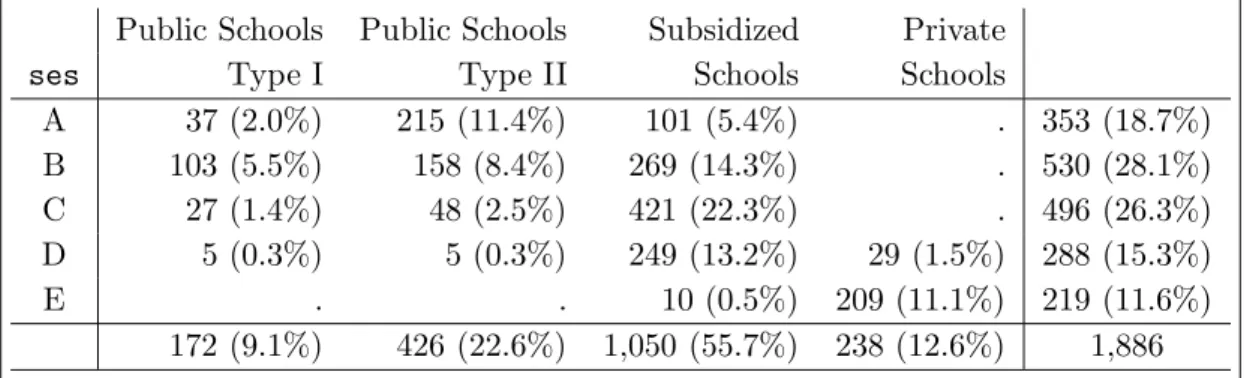
The dataset used in this study correspond to the 2004 and 2006 cross sections of the SIMCE test in the field of Mathematics. In 2004, the test was applied to 276,365 students from the 8th level. In 2006 most of the tested students were at the 10-th level. Using the unique national identity card, it was possible to link both cross sections at the student level, obtaining thus a panel of 177,463 students over two periods of time. We also limited the data set in considering schools with at least 20 students. The final dataset considered in our study contains 163,286 students spread in 1,886 schools. Of these, 9.1% are Public Schools of Type I, 22.6% are Public Schools of Type II; 55.7% are Subsidized Schools; and 12.6% are Private Schools.

The Chilean Ministry of Education defines the socio-economic status of the schools (herewith denoted by ses_{) taking into account regularly collected information at school}

level. Five ordered levels are defined from A to E, level A being the lowest socio-economic level. Of the 1,886 schools, 353 (i.e. 18.7%) are classified at level A; 530 (i.e. 28.1%) at level B; 496 (i.e. 26.3%) at level C; 288 (i.e. 15.3%) at level D; and 219 (i.e. 11.6%) at level

(8)

Table 1: Number of Schools by Type of School and Socio-economic Status

Public Schools Public Schools Subsidized Private

ses _{Type I} _{Type II} _Schools _Schools

A 37 (2.0%) 215 (11.4%) 101 (5.4%) . 353 (18.7%) B 103 (5.5%) 158 (8.4%) 269 (14.3%) . 530 (28.1%) C 27 (1.4%) 48 (2.5%) 421 (22.3%) . 496 (26.3%) D 5 (0.3%) 5 (0.3%) 249 (13.2%) 29 (1.5%) 288 (15.3%) E . . 10 (0.5%) 209 (11.1%) 219 (11.6%) 172 (9.1%) 426 (22.6%) 1,050 (55.7%) 238 (12.6%) 1,886

Table 2: SIMCE Mathematics performance by Type of School

Type of Number of Mean S.D. Mean S.D. School Students mat06 mat06 mat04 mat04

Public Schools I 22,799 (14.0%) 245.8 64.6 253.5 48.5 Public Schools II 50,918 (31.2%) 241.8 61.1 251.1 46.9 Subsidized Schools 77,314 (47.3%) 263.5 61.9 264.7 47.0 Private School 12,255 (7.5%) 331.7 47.1 315.4 40.8

E. Table 1 shows the number and percentage of schools by both socio-economic status and type of schools.

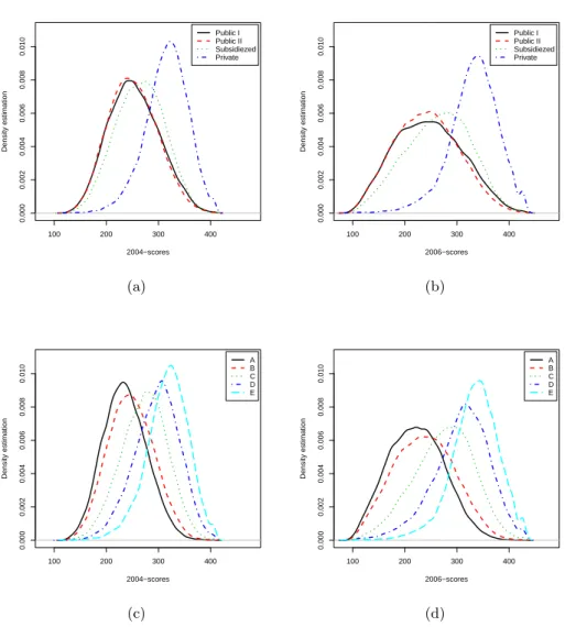
The SIMCE-scores of students were estimated by the SIMCE office from the Chilean Ministry of Education using a 2PL model; for details on this model model, see Embretson and Reise (2000). Tables 2 and 3 show a summary of the scores of the students controlled by type of school and by socio-economic status of the school, respectively. In tables,mat04_and mat06_{denote the score in the field of Mathematics obtained in 2004 and 2006, respectively.}

It can be noticed a significant relationship between socio-economic status and Mathematics performance. This feature has already been established in other studies for school achieve-ment, such as the PISA test (OECD, 2007, Chapter4). This information is complemented with Gaussian kernel density estimators of the corresponding scores as shown in Figure 1; the bandwidths were chosen using the rule-of thumb as introduced by Silverman (1986, p. 48). For panel (a) in Figure 1, the bandwidths are equal to 5.86 (Public I schools), 4.83 (Public II schools), 4.45 (Subsidized schools) and 5.37 (Private schools). For panel (b), 7.81 (Public I schools), 6.29 (Public II schools), 5.87 (Subsidized schools) and 5.92 (Private schools). For panel (c), 4.79 (SES A), 4.36 (SES B), 4.70 (SES C), 5.48 (SES D) and 5.37 (SES E). For panel (d), 6.14 (SES A), 5.77 (SES B), 6.09 (SES C), 6.47 (SES D) and 5.89 (SES E).

3.2 Description of the covariates

Together with the application of SIMCE test, a questionnaire is applied to parents in order to collect socio-demographic information. At the individual level, the following covariates

(9)

Table 3: SIMCE Mathematics performance by School Socioeconomic Status ses _{Number of} _Mean _S.D. _Mean _S.D.

Students mat06 mat06 mat04 mat04

A 29,369 222.5 53.4 236.3 41.6 B 60,143 237.2 57.9 247.3 43.8 C 43,600 274.3 57.3 272.9 44.2 D 18,649 308.3 53.9 296.7 43.5 E 11,525 333.7 45.7 316.8 40.3 100 200 300 400 0.000 0.002 0.004 0.006 0.008 0.010 2004−scores Density estimation Public I Public II Subsidiezed Private (a) 100 200 300 400 0.000 0.002 0.004 0.006 0.008 0.010 2006−scores Density estimation Public I Public II Subsidiezed Private (b) 100 200 300 400 0.000 0.002 0.004 0.006 0.008 0.010 2004−scores Density estimation A B C D E (c) 100 200 300 400 0.000 0.002 0.004 0.006 0.008 0.010 2006−scores Density estimation A B C D E (d)

Figure 1: Gaussian kernel density estimators for the 2004- and 2006-scores distributions

(10)

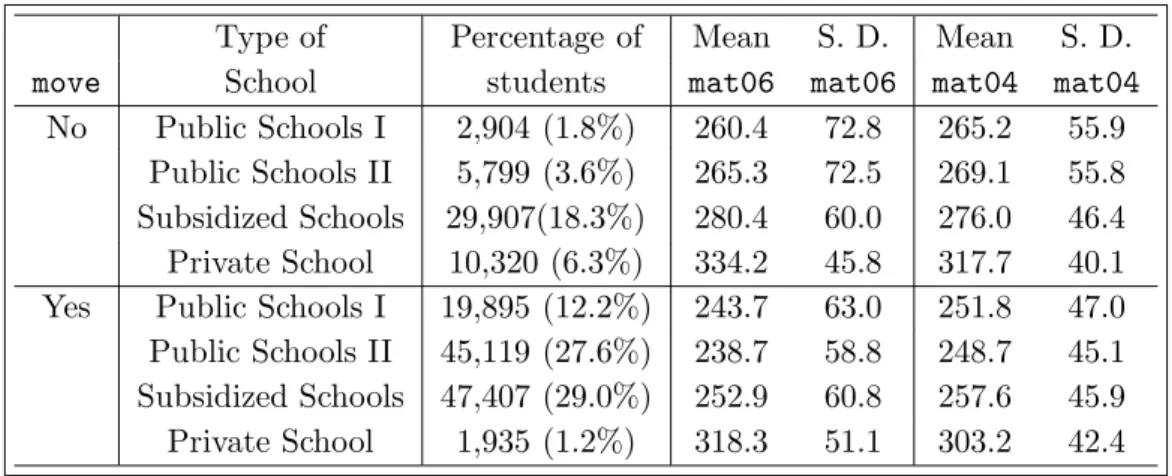
Table 4: Student school movement between 2004 and 2006

Type of Percentage of Mean S. D. Mean S. D.

move _School _students mat06 mat06 mat04 mat04

No Public Schools I 2,904 (1.8%) 260.4 72.8 265.2 55.9 Public Schools II 5,799 (3.6%) 265.3 72.5 269.1 55.8 Subsidized Schools 29,907(18.3%) 280.4 60.0 276.0 46.4 Private School 10,320 (6.3%) 334.2 45.8 317.7 40.1 Yes Public Schools I 19,895 (12.2%) 243.7 63.0 251.8 47.0 Public Schools II 45,119 (27.6%) 238.7 58.8 248.7 45.1 Subsidized Schools 47,407 (29.0%) 252.9 60.8 257.6 45.9 Private School 1,935 (1.2%) 318.3 51.1 303.2 42.4

are collected:

1. Mother’s educational level (mothed_{) and father’s educational level (}fathed_{). Parents}

are asked to indicate the last completed educational level. An educational level of 0 year means no education. Primary school is between 1 and 8 years; secondary school is between 9 and 12 years; technical secondary school is 13 years; technical professional school is 14 or 15 years; incomplete university education is 16 years; complete university level is 17 years; master level is 18 years; and PhD level is 19 years.

2. Student school movement indicator (move). This is a categorical variable indicating

whether a student moved from a school to another school between 2004 and 2006. As Table 4 shows, 70% of students moved between 2004 and 2006. This mobility is due in part to the fact that most schools attended by students at 2004 organized studies at the primary level only. Therefore those students were obliged to change school between the two periods of testing.

3. Student fall indicator (fall_{). This is a categorical variable, which indicates whether}

a student had to repeat a grade in the past before 2006. 4. Gender.

At the school level, the following covariables were available: 1. Socio-economic status of the school (ses_{) (above-described).}

2. Selectivity of the school (select_{). A selectivity mechanism widely used by schools}

is the selectivity by ability. In their questionnaire, parents are asked whether a test of knowledge on their child was organized when they applied for the school. Schools which use this mechanism of selection are free to decide whom to apply such a test. For each school,select_{corresponds to the proportion of questionnaires which report}

(11)

4 Statistical Analysis by Instrumental Mixed Modeling

4.1 A Definition of the value-added

Since our database contains two cross-sections, a possible approach to measure the effective-ness of schools is to compute their so-calledvalue-added. Value-added measures the gain (or loss) of being in a given school and is based on the student progress. It therefore requires at least one lagged measure of the score representing a baseline. Progression of students in each schools are then compared jointly, that is the gain (or loss) of being educated in a given school is calculated with respect to an “average” school; see Raudenbush and Willms (1995); Raudenbush (2004) and OECD (2008, pp.16-17).

In order to formalize that notion we denote bymat06_ij _{the observed score in mathematics}

in 2006 for pupilibelonging to schoolj, and by mat04_ij _{the lagged score in 2006. All other}

covariates, being school-specific or not, are denoted by the vectorXij. In addition to those

covariates, we also have the possibility to control for the school selectivity by adding other covariates. A natural candidate is to take the average of mat04_ij _{over students in each}

schoolj as a possible control variable. That variable is below denoted byavmat04_j _{and will}

be showed to satisfactorily control for the unobserved selectivity process of schools.

The random effect of schooljis denoted byθj. By definition this latent variable controls

for school-heterogeneity and thus represents unobserved school-specific characteristics that may include both school practices (on which school have some control) and school contexts (Raudenbush, 2004). With these notations, the value-added is the measure of the following difference : VAj = 1 nj nj X i=1

E(mat06_ij _|mat04_ij_,avmat04_j_{, X}_X_X_ij_{, θ}_j₎ ₋

(1) 1 nj nj X i=1

E(mat06_ij _|mat04_ij_,avmat04_j_{, X}_X_X_ij₎_,

where nj is the number of pupils belonging to school j. The first term is the average of

the expected scores given the specific characteristics of school j when controlling for the lagged score, the selectivity and all other covariates. The second term integrates out the school-specific effect and therefore represents the average of expected scores of an average school given the covariates.

The practical computation of these expectations are based on a specific model that must be assumed on the score. Hierarchical linear mixed (HLM) models appear to be a widely used standard in the topic of educational assessment. It assumes the following specification:

mat06_ij ₌_X′

ijβ+γmat04ij+αavmat04j+θj+ǫij, (2)

whereβis a vector of parameter (we have modeled the intercept as the first element ofβ),γ

is the parameter of the lagged score, andǫij are independent errors, possibly heteroscedastic

and often assumed to be zero-mean and normally distributed. If the school random effect

(12)

expectation E(θj |mat04ij,avmat04j, XXXij) vanishes and we find that

VAj = θj

(3) = E(mat06_ij _|mat04_ij_,avmat04_j_{, X}_X_X_ij_{, θ}_j₎₋_E₍mat06_ij _|mat04_ij_,avmat04_j_{, X}_X_X_ij₎

for alli; that is, the value-added of schoolj is given by the random effectθj. This equality

makes explicit the structural meaning of the random effect θj and actually explains why

and in which sense it is a representation of the value-added of school j. In this setting, the value-added is computed as the predictor of the random effect, as typically done in this type of literature; see e.g. Raudenbush and Willms (1995); Goldstein and Spiegelhalter (1996); Goldstein and Thomas (1996); Tekweet al. (2004); Hutchisonet al. (2005).

4.2 Results from a standard valued-added analysis

In a preliminary analysis, a homoscedastic HLM model has been fitted to the SIMCE data. However, after residual analysis controlling by the socio-economic status of the schools, it was concluded that the normality assumption of the random effect is violated. We therefore run the valued-added analysis by fitting a heteroscedastic HLM models in which the variance of θj and ǫij may depend on the socio-economic level of the school. More specifically, the

variance structure in (2) is supposed to be such that

V ar(Yij |mat04ij,avmat04j, XXXij, θj) =σ2_ρ₍_j₎ for all studentsibelonging to schoolj,

V ar(θj |mat04ij,avmat04j, XXXij) =τ_ρ2₍_j₎,

whereρis a function that mapsjinto the socioeconomic status of schoolj; that is,ρ(j) =A

if the socio-economic status of the schooljisA, and so on. In agreement with this structure, the conditional model of Yij given mat04ij,avmat04j, XXXij and θj was specified with an

intercept for each socio-economic level using the covariateses_.

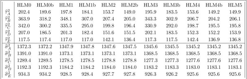
The initial within-variances are _bτ_A2 = 1,313.1; _bτ_B2 = 1,109.3; _bτ_C2 = 1,412.2; _bτ_D2 = 3,586.1; and _bτ_E2 = 7,388.4; and the initial between-variances are σ_b_A2 = 2,433.9; _bσ_B2 = 2,515.9; σ_b2_C = 2,411.4; σ_b2_D = 2,202.2; _bσ_E2 = 1,831.1. Once it is controlled by the baseline score mat04_{, along with an intercept by each socio-economic level, both the within and}

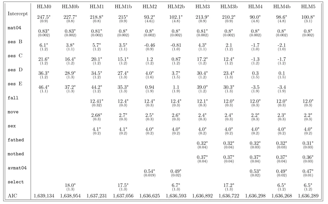
between variances decrease dramatically. Nine specifications were fitted and are summarized in Table 6. The reference for ses _{is the socio-economic status A; the reference for} fall

is “the student fells in the past”; the reference for move_{is “the student did move between}

2004 and 2006”; and the reference for sex_{is “woman”.}

As we mentionned above, the covariate avmat04 _{is a relevant control variable for the}

unobserved selectivity of schools. By “unobserved” selectivity, we refer to a selectivity bias that is not self reported by the parents through the covariateselect_{. We now give empirical}

arguments supporting that choice.

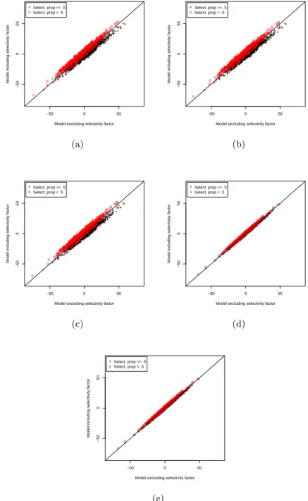
First, we show the existence of a selectivity bias in the sample. For this, we can compare the value-added obtained from HLM models that do not contain select _{with the}

value-added that is obtained when we add this covariate. In Table 6, we therefore compare HLM0 with HLM0b, HLM1 with HLM1b and so on. The five pictures of Figure 2 show

(13)

the comparison of the value-added for the five HLM models. In the plot, value-added in black color correspond to schools that are such that select > 50%, that is, they have a high reported selectivity. Red value-added are the other schools, having a low reported selectivity. In general, these figures show that highly selective schools (in black) have higher value-added if select _{is not included in the HLM model. Conversely, the value-added of}

less selective schools (in red) have lower value-added ifselect_{is not included in the model.}

Consequently, the exclusion of select _{as a covariate benefits the schools which select at}

least 50% of the students; and the inclusion ofselect _{benefits the schools which select at}

most 50% of the students.

To see now how avmat04 _{helps in controlling the selectivity bias, compare pictures (b)}

to (e) in Figure Figure 2. We see that the inclusion of avmat04 _{as a covariate decreases}

the distance between these two types of schools and, therefore, the inclusion/exclusion of

selectas a covariate is successfully controlled. The same conclusions can be drawn if the

comparisons are done between schools of the same type (namely, public schools type I; type II; subsidized; and private).

(14)

Table 5: Results from classical Value-Added analysis HLM0 HLM0b HLM1 HLM1b HLM2 HLM2b HLM3 HLM3b HLM4 HLM4b HLM5 Intercept 247.5∗ _227.7∗ _218.8∗ ₂₁₅∗ _93.2∗ _102.1∗ _213.9∗ _210.2∗ _90.0∗ _98.6∗ _100.8∗ (0.9) (0.8) (0.8) (0.9) (4.6)) (4.8) (0.9) (0.9) (4.8) (4.8) (3.1) mat04 0.83∗ _0.83∗ _0.81∗ _0.8∗ _0.8∗ _0.8∗ _0.81∗ _0.8∗ _0.8∗ _0.8∗ _0.8∗ (0.002) (0.002) (0.002) (0.002) (0.002) (0.002) (0.002) (0.002) (0.002) (0.002) (0.002) ses _B 6.1∗ _3.8∗ _5.7∗ _3.5∗ _-0.46 _-0.81 _4.3∗ _2.1 _-1.7 _-2.1 (1.2) (1.1) (1.2) (1.1) (0.9) (1.0) (1.1) (1.2) (1.0) (1.0) ses _C 21.6∗ _16.4∗ _20.1∗ _15.1∗ _1.2 _0.87 _17.2∗ _12.4∗ _-1.3 _-1.7 (1.2) (1.2) (1.2) (1.2) (1.2) (1.2) (1.2) (1.2) (1.2) (1.2) ses _D 36.3∗ _28.9∗ _34.5∗ _27.4∗ _4.0∗ _3.7∗ _30.4∗ _23.4∗ _0.3 _0.1 (1.2) (1.3) (1.2) (1.3) (1.6) (1.5) (1.2) (1.3) (1.5) (1.5) ses E 46.4∗ _37.2∗ _44.2∗ _35.3∗ _0.94 _1.1 _39.0∗ _30.3∗ _-3.5 _-3.4 (1.1) (1.3) (1.2) (1.3) (1.9) (1.9) (1.2) (1.3) (1.9) (1.9) fall 12.41∗ _12.4∗ _12.4∗ _12.4∗ _12.1∗ _12.0∗ _12.0∗ _12.0∗ _12.0∗ (0.32) (0.3) (0.3) (0.3) (0.3) (0.3) (0.3) (0.3) (0.3) move 2.68∗ _2.7∗ _2.5∗ _2.6∗ _2.4∗ _2.4∗ _2.2∗ _2.3∗ _2.2∗ (0.3) (0.3) (0.3) (0.3) (0.3) (0.3) (0.3) (0.3) (0.3) sex 4.1∗ _4.1∗ _4.0∗ _4.0∗ _4.0∗ _4.0∗ _4.0∗ _4.0∗ _4.0∗ (0.2) (0.2) (0.2) (0.2) (0.2) (0.2) (0.2) (0.2) (0.2) fathed 0.32∗ _0.32∗ _0.32∗ _0.32∗ _0.31∗ (0.04) (0.04) (0.03) (0.03) (0.03) mothed 0.37∗ _0.37∗ _0.37∗ _0.37∗ _0.36∗ (0.04) (0.04) (0.04) (0.04) (0.03) avmat04 0.54∗ _0.49∗ _0.53∗ _0.49∗ _0.47∗ (0.019) (0.02) (0.02) (0.02) (0.01) select 18.0∗ _17.5∗ _6.7∗ _17.2∗ _6.5∗ _6.5∗ (1.3) (1.3) (1.3) (1.3) (1.2) (1.2) 12

(15)

Table 6: Results from classical Value-Added analysis (Continued) HLM0 HLM0b HLM1 HLM1b HLM2 HLM2b HLM3 HLM3b HLM4 HLM4b HLM5 b τ_A2 202.4 189.6 197.8 184.1 153.7 149.0 195.9 183.5 153.6 149.2 149.9 b τ_B2 363.9 318.2 348.1 307.0 207.4 205.0 343.3 302.9 206.7 204.2 206.1 b τ_C2 342.0 300.2 335.5 295.0 199.8 196.4 330.9 292.0 198.7 195.5 195.8 b τ_D2 207.0 186.5 201.3 182.4 151.6 151.5 202.1 183.5 152.3 152.2 153.9 b τ_E2 117.5 117.4 117.0 117.0 142.1 136.4 117.3 117.5 142.4 136.9 136.8 b σ_A2 1372.3 1372.2 1347.9 1347.8 1347.6 1347.5 1345.6 1345.5 1345.2 1345.2 1345.2 b σ_B2 1391.0 1391.0 1373.1 1373.1 1373.1 1373.1 1368.5 1368.5 1368.5 1368.5 1368.5 b σ_C2 1289.4 1289.5 1278.5 1278.5 1278.8 1278.8 1277.3 1277.3 1277.6 1277.6 1277.6 b σ_D2 1192.3 1192.3 1184.2 1184.2 1184.0 1184.0 1183.2 1183.3 1183.0 1183.1 1183.1 b σ_E2 934.3 934.2 928.5 928.4 927.7 927.8 926.3 926.2 925.6 925.6 925.6 13

(16)

The fixed effects corresponding to the covariates at the individual level are stable across the different models (when the covariate is included): around 0.8 for mat04_{; around 12.0}

for fall _{(the coefficient is positive for students who did not fall in the past); around 2.2}

formove_{(the coefficient is positive for students who did not move between 2004 and 2006);}

around 4.0 forsex_{(the coefficient is positive for men); around 0.32 for} fathed_{and 0.37 for} mothed_.

With respect to the fixed effects at the school level, the coefficient of select_{is around}

17.0 whenavmat04_{is not included in the model; when it is included, the coefficient of}select

is around 6.5, whereas the coefficient of avmat04 _{is around 0.50. This also quantifies how} avmat04 _{controls the selectivity of the school. With respect to the socio-economic level of}

the school, the type III test (computed by PROC MIXED of SAS) is significative in all models. Furthermore, when the t-test corresponding to each category of ses _{is significant,}

the fixed effect for level B is between 3.5 and 6.1; for level C between 12.4 and 21.6; for level D, between 23.4 and 36.3; and for level E, between 30.3 and 46.4. However, when

avmat04_{is included in the model (in HLM2, HLM2b, HLM4 and HLM4b models), some (if}

not all) of the categories ofses_{are non significant. Taking into account the AIC-criterion,}

the model HLM4b is the best model although the four categories ofses_{are non significant.}

From the above analysis, we keep model HLM5 as the baseline for the following steps of our analysis below.

4.3 The endogeneity of some covariables

Although the previous analysis follows a classical approach to compute the value-added, our description above emphasizes that it relates to structural assumptions, among which the most critical is certainly the independence between the random effectθj and all covariates.

Recall that mat04_ij _{represents the lagged version of the score and} avmat04_j _denotes

its average over schools. It is likely that these two covariates already contain the effect of the school, particularly if studentialready belongs to schoolj at that time. Independence between the school effectθj and variablesmat04ij oravmat04jis therefore questionable, and

it raises the important statistical question of what corrections on the value-added calculation should we apply if this assumption is not fulfilled.

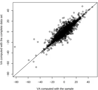
It is possible to support this observation from the SIMCE data. Over all students kept in the database, 70% have moved between 2004 and 2006. The reason of moving may be due to the choice of the parents, or may be unavoidable due to the school system itself. Let us consider the HLM model and the value-added of schools that are calculated from the subsample of moving students only. In Figure 3 we compare this value-added with the value-added that is calculated from the whole sample. Both calculations are based on the HLM5 specification. A high variation is observed between the two calculations, leading to important differences in the school ranking. To quantify that last point, we notice that the Spearman correlation between the two value-added predictions is 0.873.

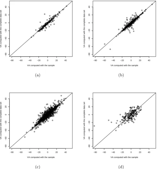
To have a better picture of what happened, it is useful to compare this difference ac-cording to the school type. As we can observe from the above Table 4, the moving rate is variable according to the type of school considered: it is 16% for Private Schools, 61% for Subsidized Schools, 87% for Public Schools Type II and 89% for Public Schools Type

(17)

+ + + + + + + + + + + + + ++ + + + + + + + + + ++ + + + + + + + + + + + + + ++ + + + + + + + + + + + + + + + ++ + + + + + + + + + + + + + + + + + + + + + + + + + + + + + ++ + + + + + + + + ++ + + + + + + + + + ++ ++ ++ + + + + +++ + + + + + + + + + + + + + + ++ + + + + + + + + ++ + + + + + ++ + + + + + + + + + + + + + + + + + + + + ++ + + + + + + + + + + + + + + + + + + + + ++++ + + + + + + + + + + + + + + + + ++ ++ + + + + + + + ++ + + + + + + ++ + + + + + + + + + + + ++ ++ + + + ++ + + + + + + + ++ + + + + ++ + + + + + + + + + + + + + ++ + + + + ++ + + +₊+ + + + + + + + + + + + + + + + + + + + + + + + + + + + + + + + + + + ++ + + + + + + + + + + + + + + + + + + ++ + + + + + + + + + + + + + + + + + + + + ++ + + + + + + + + + + ++ + ++ + +++ + + + + + + + ++ +++ + ++ + + + + + + ++ + + + + + ++ + + + + + + + + + + + + + + + + + ++ + + + + + + + + + + + + + + + + + + + + + + + +₊ + + + + + ++ + + + ++ + + + + + + + + ++ + + + ++ + + + ++ + + + + + + +++ + + + + + + + + + + + + + + + + + + + + + + + + + + + + + + + + + + + + + + + + + + + + + + + + + + + ++ + + + + + + + + + + + + ++ + + + + + + + + + ++ + + + + + + + + + + + + + + + + + + + + + + ++ + + ++++ + + + + + + + + + + + + + + + + + ++ + ++ + + + + + + + + + + + + + + + + + + + + + + + + + + + + + + + + ++ + + + ++ + + + + + + + + + + + + + + + + + + + + + + + + + + + + + + + + + + + + + + + + + + + + + + + + + + + + + + + + + + + + + + + + + + + + + + + + ++ + + + +₊ + ++ + + + + + + + + ++ + + + + ++ + + + + + + + + + + + + + + + + + + + + + + ++ ++ + + + + + + + + + + + + + + +++ + ++ + + + + + + + + + + + + + + ++ + + + + + + + + + + + + + ++ + +++ + + + + + + + + + + + + + + ++ + ++ + + + + + + + + + + + + + + + + + + + + + + + + + + + +++ + + + + + + + + + + + + + + −50 0 50 −50 0 50

Model excluding selectivity factor

Model including selectivity f

actor o o o o o o o o o o o o o o o o o o oo o o o o o o o oo o o o o o o oo o o o o o o o o o o o o o o o o oo o o oo o o o o o o o o o o o o o o o o o o oo o o o o oo o o o o o o o o o o oo oo o o o o o o o o o o o o o o oo o o o oo o o o o o o oo o o oooo o o o oo o o o o o o o o o o o o o o o o o o o o o o o o o o o o o o o o o o o o o o o o o o o o o oo o o o o o o o o o o o o o oo o o o ooo o o o o oo o o o o o o o o o o oo o o o o o o o o o o o o o o o o o o o o o o oo o o o o ooo ooo o o o o o o o o o oo o o o o o o o o o oo oo o o o o oo o o o o o o o o o o oo o o o o o o o o o o o o o o o o o o o o o o o o o o o o o o o o o o o o o o o o o oo o o o o o o o o o o o o o o o o o o o o o o o o o o o o o o o o o o o o oo oo o oo o o o o oo o o o o o o o o o o o o o oo o o o o o o o o o o o o o o o o o o o o o o oo o o o o o o o o o o o o o oo o o oo o o oo o o oo o o o o o o o o o o o o o o o o o o oo o o o o o o o o o o o oo o o o o o o o o o o o o oo o o o o o o o o o o o o o o o o o o o o oo o o o o o oo o o o o o o o o o o o o o o o o o o o o o o o o o o o o o o o o o o oo o o o o o o o o o o o o o o o o o o oo o o oo o o o o o o o o o o o oo o o o o o o o o o o o o o o o o o o o o o o o oo o o o o o o oo o o o o o o oo o o o o o o o o o o o o o o o o o oo o o o o oo o o oo o o oo o o o o o o o o o o o o o o o o o o o o o o o o o o o o o o o ooo o o o o o o o o o o o oo o o o oo o o o o oo o o o o o o o o o o o o o o o o o oo o o o o o o o o o o o o oo o o o o o o o o o o o o o o o o o o o o o o o o o o o o o o o o o o o o o o o o o o o oo o o oo o o o o o o o o o o o o o o o o o o o o o o o o o o o o o o o o o o o o o o o o o o o oo o o o o o o o o o o ooo o o o o o o o o o o o o o o o o o o o o o o o o o o o o o o o o o o o o o o o o o o o o oo o o o o oo o o o o o oo o o o o o o o o o o oo o o o o o o o o o o o o o o + o Select. prop >= .5 Select. prop < .5 (a) + + + + + + + + + + + + + ++ + + + + + + + + + ++ + + + ++ + + + + + + + + ++ + + + + + + + + + + + + + + + ++ + + + + + + + + + ++ + + + + + + + + + + + + + + + + ++ + + + + + + + + + + ++ + + + + + + + + +++ + + + + + + + + + + + + + + + + + + + + + + + + + ++++ ++ + + + + + + + + + + + + + + + + + + + + + + + + + + + + + + + + + ++ + + + + + + + + + + + + + + + + + + + + ++++ + + + + + + + + + + + + + + + + ++ +++ + + ++ + + ++ + + + + + + ++ + + + + + + + + + + + ++ + + + + + + + + + + + + + + ++ + + + + ++ + + + + + + + + + + + + + + + + + + + ++ + + +₊+ + + + + + + + + + + + + + + + + + + + + + + + + + + + + + + + + + + ++ + + + + + + + + + + + + + + + + + + ++ + + + + + + + + + + + + + + + + + + + + ++ + + + + ++ + + + + ++ + ++ + +++ + + + + + + + + + + ++ + ++ + + + + + + + + + + + + + ++ + + + + + + + + + + + + + + + + + ++ + + + + + + + + + + + ++ + + + + + + + + + + + + + + + + + ++ + + + + + + + + + + + + + + + + + + +₊ + + + ++ + + + ++ + +++ + + + + + + + + + + + + + + + + + + + + + + + + + + + + + + + + + + + + + + + + + + + + + + ++ + + + + + + + + + + + + + + + + + + + + + + + + + + + + ++ + + + + + + ++ + + + + + + + + + + + + + + +++ + +++ + + + + + + + + + + + + + + + + + + ++ + ++ + + + + + + + + + + ++ + + + + + + + + + + + + + + + + + + + + + + + + + ++ + + + + + + + + + + + + + + + + + + + + + + + + + + + + + + + + + + + + + ++ + + + ++ + + + + +₊ + + + + + + + + + ++ + + + + + + + + + + + ++ + + + + + + + + + + + + + + + + ++ + + + + + + + + + + + + + + + + + + + + ++ + +++ + + ++ ++ + + + + + + + + + + + + + + ++ + + ++ + ++ + + + + + + + + + + + ++ + + + + + + + + + + + + + ++ + + + ++ + + + + + + + + + + + + + ++ + + + + + + + + + + + ++ + + + + + + + + + + + + + + + + + +++ + + + + + + + + + + + + + + −50 0 50 −50 0 50

actor o o o o o o o o o o o o o o o o oo oo o o o o o o o oo o o o o o o o o o o o o o o o o o o o o o o o o o oo o oo o o o o o o o o o o o o o o o o o o oo o o o o oo o o o oo o o o o o oo oo o o o o o o o o o o o o o o oo o o o o o o o o o o o oo o o oooo o o o oo o oo o o o o oo o o o o o o o o o o o o o o o o o o o o o oo o o o o o o o o o o o o o o o o o o o o o o o o o o o o oo o o o ooo o o o o oo o o o o o o o o o o oo o o o o o o o o o o o o o o o o o o o o o o oo o o o o o oo ooo o o o o o o o o o o o o o o o o o o o o o o oo o o o o oo o o o o o o o o o o oo o o oo o o o o o o o o o o o o o o o o o o o o oo o o o o o o o o o o o o o o o oo o o o o o oo o o o o o o oo o o o o o o o o o o o o o o o o o o o o ooo oo o oo o o o o oo o o o oo o o o o o o o o oo o o o o o o o o o o o o o o o o o o o oo o oo o o o o o o o o o o o o o o o o o o o o o oo o o oo o o o o o o o o o o o o o o o o o o oo o o o o o o o o o o o o o o o o o o_o o o o o o o oo o o o o o o o o o o o o o o o o o o o o o o o o o o o o o o o o o o o o o o o o o o o o o o o o o o o o o o o o o o o o o o o o o o o o o o o o o o o o o o o o o o o o o o o oo o o o o o o o o o o o o o o o o o oo o o o o o o o o o o o o o o o o o o o o o o o o o oo o o o o o o o o o o o o o o o o o o o o o o o o o oo o o o o oo o o o o o o oo o o o o o o o o o o o o o o o o o o o o o o o o o o o o o o o o oo o o o o o o o o o o o oo o o o oo o ooo oo o o o o o o o o o o o o o o o o o o o o o o o o o o o o_o o o o o o o o o o o o o o o o o o o o o o o o o o o o o o o o o oo o o o o o o o o o o o o o oo o o oo o o o o o o o oo o o o o o o o o o o o o o o o o o o o o o o o o o o o o o o o o o o o o o o o o o o oo o o ooo oo_o o o ooo o o o o o o o o o o o o o o o o o o o o o o o o o o o o o o o o o o o oo o o o o o oo o o o o o oo o o o o o o o o o o o o o o o o o o o o o o o o o o + o Select. prop >= .5 Select. prop < .5 (b) + + + + + + + + + + + + + ++ + + + + + + + + + ++ + + + + + + + + + + + + + ++ + + + + + + + + + + + + + + + ++ + + + + + + + + + + + + + + + + + + + + + + + + + + + ++ ++ + + + + + + + + ++ + + + + ++ + + + ++ ++ + + + + + + +++ + + + + + + + + + + + + + + ++ ++ ++ + + + + + + + + + + + ++ + + + + + + + + + + + + + + + + + + + + ++ + + + + + + ++ + + + + + + + + + + + + + ++ + + + ++ + + + + + + + + + + + + ++ +++ + + ++ + + ++ + + + + + + ++ + + + + + + + + + + + ++ + + + + + + + + + + + + + + ++ + + + + + + + + + + + + + + + + + + + + + + + + + ++ + + +++ + + + + + + + + + + + + + + + + + + + + + + + + + + + + + + + + + + + ++ + + + + + + + + + + + + + + + + + ++ + + + + + + + + + + + + ++ + + + + + + ++ + + + + ++ + + + + ++ + ++ + +++ + + + + + + + + + + ++ + ++ + + + + + + + + + + + + + ++ + + + + + + + + + + + + + + + + + ++ + + + + + + + + + + + ++ + + + + + + + + + + + + + + + + + ++ + + + ++ + + + + + + + + ++ + + + +₊ + + + ++ + + ++ + + +++ + + + + + + + + + + + + + + + + ++ + + + + + + + + + + + + + + + + + + + + + + + + + + + + ++ + + ++ + + + + + + + + + + + + + + + + + + + + + + + + ++ + + + + + + ++ + + + + + + + + + + + + + + +++ + ++++ + + + + + + + + + + ++ + + + + + ++ + ++ + + + + + + + + + + ++ + + + + + + + + + + + + + + + + + + + + + + + + + ++ + + + + + + + + + + + + + + + + + + + + + + + + + + + + + + + + + + + + + ++ + + + ++ + + ++ +₊ + + + + + + + + + ++ + + + + + + + + + + + ++ + + + + + + ++ + + + + + + + + ++ + + + + + + + + + + + + + + + + + + + + ++ + + + + + + ++ ++ + + + + + + + + + + + + + + +++ + ++ + ++ + + + + + + + + + + + ++ + + + + + ++ + + + + + + ++ + + + ++ + + + + + + + + + + + + + ++ + ++ + + + + + + + + ++ + + + + + + + + + + + + + + + + + +++ + + + + + + + + + + + + + + −50 0 50 −50 0 50

actor o o o o o o o o o o o o o o o o oo oo o o o o o o o oo o o o o o o o o o o o o o o o o o o o o o o o o o oo o oo o o o o o o o o o o o o o o o o o o oo o o o o o o o o o oo o o o o o oo oo o o o o o o o o o o o o o o oo o o o o o o o o o o o oo o o o ooo o o o oo o oo o o o o oo o o o o o o o o o o o o o o o o o o o o o o o o o o o o o o o o o o o o o o o o o o o o o o o o o o o oo o o o ooo o o o o oo o o o o o o o o o o oo o o o o o o o o o o o o o o o o o o o o o o o o o o o o o oo ooo o o o o o o o o o oo o o o o o o o o o oo oo o o o o o o o o o o o o o o o o oo o o oo o o o o o o o o o o o o o o o o o o o o o o o o o o o o o o o o o o o o o oo o o o o o oo o o o o o o oo o o o o o o oo o o o o o o o o o o o o ooo ooo oo o o o o oo o o o o o o o o o o o o o oo oo o o o o o o o o o o o o o o o o o o_o o oo o o o o o oo o o o o o o o o o o o o o o oo o ooo o o o o o o o o o o o o o o o o o o oo o o o o o o o o o o o o o o o o o o o o o o o o o oo o o o o o o o o o o o o o o o o o o o o o o o o o o o o o o o o o o o o o o o o o o o o o o o o o o o o o o o o o o o o o o o oo o o o o o o o o o o o o o o o o o o oo o o oo o o o o o o o o o o o oo o o o o oo o o o o o o o o o o o o o o o o o o o o o o o o o oo oo o o o o o o o o o o o o o o o o o o o o o o o oo o o o o oo o o o o o o oo o o o o o o o o o o o o o o o o o o o o o o o o o o o o o o o o oo o o o o o o o o o o o oo o o o oo o ooo oo o o o o o o o o o o o o o o o o o oo o o o o o o o o o o o o o o o o o o o o o o o o o o o o o o o o o o o o o o o o o o oo o o o o o o o o o o o o o oo o o oo o o o o o o o oo o o o o o o o o o o o o o o o o o o o o o o o o o o o o o o o o o o o o o o o o o o oo o o ooo o o o o o o oo o o o o o o o o o o o o o o o o o o o o o o o o o o o o o o o o o o o o oo o o o o oo o o o o o ooo o o o o o o o o o o o o o o o o o o o o o o o o o + o Select. prop >= .5 Select. prop < .5 (c) + +++ + ++ ++ + + ++ + + + + + + + + + + ++ + + + + + + + + + + + + ++ + + + + + + + + + + + + + + + + + ++ + + + + + + + + + ++ + + + + + + + ++ + + + + + + ++ + + + + + + + + + + + + ++ + + ++++ + ++ + + + + + + + + + +++ + + + ++++ + + + + + + + + + ++++ + + + + +++ + + + + + + + + + + + + + + + ++ + + + +++ + + + + + + + + + + + ++ ++ + + + + ++ + + + + +++ + + + + + + + + + + + ++++ + +++ +++ + ++ + + + + + + + + + + + + + ++ + + + + + + + + + + + + + + + + + + + + + + + + + ++ + + + + + + + + ++ + + + + + ++ + + + + + + + + + + + + + + + + + + + + + + + + + + + + + ++ + + + + + + + + + + + ++ + + + + ++ + + + + ++ + + + + + + + + ++ +++ + + + + + + + + + + + + + + + + + + + + + + + + + + + + + + + +++ + + + + + + + ++ + +++ ++ ++ + + ++ + + + + + +++++ + + + ++ + + + + + + + + + + + + + + + + + + + + ++ + + + + + + + + + + ++ + + + + + + + + + + + + + + + + + + + + + + + + + + + + + + + + + + + + + ++ ++ + + + + + + + + + + + + + ++ + + + + + + + + + + + + + + + + + + + +++ + + + + ++ + ++ + + + + ++ + ++ + + + + + +++ + ++ + ++ + + + + + + + + + + + + ++ + + + + + + ++ + + + + + + ++ ++ + + + + + + + + + ++ + ++ + + + ++ + + + + + + + + + + + + + + + + + ++ + + + + + + + + + + + + + + ++ + + ++ + + + +++ ++ + + + + + ++ + ++ + + + ++ + + ++++ + + + ++ + + + + + + + + + + + + + + + + + + + + + + + ++ + ++ + ++ ++ + + ++ + + + + + ++ + + + + ++ + + + + + + + + + + + + + + + + ++ + ++ + +++ + + + + + + + + + ++ + + + + + ++ + + + + + + + + + + + + + ++ + + + ++ + + + + + + + + + + + + + + + + ++ + + + + + + + + + + + ++ + + + ++ + + + + + + + + + + + + + + + + + + + + + + + + + ++++ + + + + ++ + + + + + + + ++ ++ + + + + + + + + + ++ + + + + ++ + + +++ + + ++ + + + + + + + + + + −50 0 50 −50 0 50

actor o o o o o o o o o o o o o o o o o o o o o o o o o o o o o oo o o o o o o o o o o o o o o o oo o o o o o oo o oo oo o o o o o o oo oo o o o o oooo o ooo o oo o oo o o o o o o o o o o oo oo o oo o o oo o o o o oo o o ooo o o o o o o o o o o o o o o o o o o oo o o o o o o o o o o o o o o o o o o o o o oo o o o oo o o o o o o o o o o ooo o ooo o o ooo oo o oo o o oo o o o o o o o o o o o o o o o o o o o o o o o o o o o o o o o o o o o o o o o o o oo o o oo o oo o o oooo o o o o oo o o o ooo o oo o o o o o o o o o oo oo o o ooo o o o oo o o o o oo oo o o oo oo o o o o o oo o o oo o o o o o o o o o oo oo o o o o o o o ooo o o o o o o o o o o o oo o o o o o o o o o o ooo o o o o o o o o o o o o o o o o o o oo o o o o o o o o o oo o o o o o o o o oo oo o o o o o o o o o o o o o oo o oo o o o o o o o o o oo o o o o o o o o o o o o o o o o o oo o o o o o o o o o o o o o o o o o o oo o o o o o o o o o o o o oo o o o o o o o o o oo o o o o o o o o o o o o o o o o o ooo o o o o o o o oo o o o o o o o o o o o o o o o oo o o o oo o o o o o o o o o oo o o o o oo o o o oo o o o o o o o o o o o o o o o o o oo o o o o o o o o o o oo o oo o o o oo o oo o o o o o o o o oo o o o o oo o o oo o oo o o o o o o o o o o o o o o o o o o o o o o o o o oo o o o o o o oo o o o o o o oo o o o o ooo o o o o oo o o o o oo o o o o o oooo o oo o o o oo o o o o o o o o o o o o o o o oo o oo o o o o o o o o o o o o o o o o oo o o o o o o ooo o oo o o oo o o o o o o o o o oo o o o o o o o o o o oo o o o o oo o o o o o o o o o o o o o oo o ooo o o o oo o o o o o o o o o o o o o o o o o o o oo o o o oo o o o o o o o o o o oo oo oo o o o o oo oo o o o oo o o o o o o o o o o o o o o o oo o o o oo o o o o o o o o oo o o o o o o o o o o o o oo o o o o o o o o o o o o o o o o o o o o o o o o o o o o o o o o o o o oo + o Select. prop >= .5 Select. prop < .5 (d) + + + + + ++ ++ + + + ++ + + + + + + + + + ++ + + + + + + + + + + + + ++ + + + + + + + + + + + + + + + + + + + + + + + + + + + + ++ + + + + + + + ++ + + + + + + ++ + + + + + + + + + + + + ++ + + ++++ + ++ + + + + + + + + + ++ + + + +++ + + + + + + + + + + + ++++ + + + + ++ + + + + + + + + + + + + + + + + ++ + + + +++ + + + + + + + + + + + ++ ++ + + + + ++ + + + + +++ + + + + + + + + + + + ++++ + +++ +++ + ++ + + + + + + + + + + + + + ++ + + + + + + + + + + + + + + + + + + + + + + + + + ++ + + + + + + + + ++ + + + + + ++ + + + + + + + + + + + + + + + + + + + + + + + + + + + + + ++ + + + + + + + + + + + + + + + + + ++ + + + + ++ + + + + + + + + ++ ++ + + + + + + + + + + + + + + + + + + + + + + + + + + + + + + + + +++ + + + ++ + + ++ + + + + ++ ++ + + ++ + + + + + + + +++ + + + ++ + + + + + + + + + + + + + + + + + + + + ++ + + + + + + + + + + ++ + + + + + + + + + + + + + + + + + + + + + + + + + + + + + + + + + + + + + ++ + + + + + + + + + ++ + + + + ++ + ++ + + + + + + ++ + + + + + + + ++++ + + + + ++ + ++ + + + + ++ + ++ + + + + + +++ + ++ + ++ + + + + + + + + + + + + ++ + + + + + + ++ + + + + + + ++ ++++ + + + + + + + ++ + ++ + + + ++ + + + + + + + + + + + + + + + + + ++ + + + + + + + + + + + + + + ++ + + ++ + + + +++ ++ + + + + + ++ + ++ + + + ++ + +++ + + + + + ++ + + + + + + + + + + + + + + + + + + + + + + + ++ + ++ + ++ ++ + + ++ + + + + + ++ + + + + ++ + + + + + + + + + + + ++ + + + ++ + ++ + +++ + + + + + + + + + ++ + + + + + ++ + + + + + + + + + + + + + ++ + + + ++ + + + + + + + + + + + + + + + + ++ + + + + + + + + + + + ++ + + + ++ + + + + + + + + + + + + + + + + + + + + + + + + + ++++ + + + + ++ + + + + + + + + + ++ + + + + + + + + + ++ + + + + ++ + + + + + + + ++ + + + + + + + + + + −50 0 50 −50 0 50

actor o o o o o o o o o o o o o o o o o o o o o o o o o o o o o oo o o o o o o o o o o o o o o o oo o o o o o oo o oo oo o o o o o o oo oo o o o o oooo o ooo o oo o ooo o o o o o o o o o oo oo o oo o o oo o o o o oo o o oo o o o o o o o o o o o o o o o o o o o ooo o oo o o o o o o o o o o o o o o o o o oo o o o oo o o o o o o o o o o ooo o o o o o o o o o oo o oo o o oo o o o o o o o o o o o o o o o o o o o o o o o o o o o o o o o o o o o o o o o o o oo o o oo o oo o o oo o oo o oo oo o o o ooo o oo o o o o o o o o o oo ooo o ooo o o o oo o o o o oo oo o o o o oo o o o o o oo o o oo o o o o oo o o o oo oo o o o o o o o oo o o o o o o o o o o o o oo o o o o o o o o o o oo o o o o o o o o o o o o o o o o o o o oo o o o o o o o o ooo o o o o o o o o oo oo o o o o o o o o o o o o o oo o oo o o oo o o o o o oo o o o o o o o o o o o o o o o o o oo o o o o o o o o o o o o o o o o o o o o o o o o o o o o o o o o oo o o o o o o o o o oo o o o o o o o o o o o o o o o o o oo o o o o o o o o oo o o o o o o o o o oo o o o o oo o oooo o o o o o o o o o oo o o o o o o o o o oo o o o o o o o o o o o o o o o o o oo o o o o o o o oo o oo o oo o o o oo o oo o o o o o o o o oo o o o o o o o o oo o oo o o o o o o o o o o o o o o o o o o o o o o o o o o o o o o o o o oo o o o o o o oo o o o o ooo o o o o oo o o o o oo o o o o o oooo o o o o o o oo o o o o o o o o o o o o o o o oo o o o o o o o o o o o o o o o o o o o oo o o o o o o ooo o oo o o oo o o o o o o o o o oo o o o o o o o o o o oo o o o o oo o o o o o o o o o o o o o oo o o oo o o o o o o o o o o o o o o o o o o o o o o o o oo o o o oo o o o o o o o oo o oo oo oo o o o o o o oo o o o oo o o o o o o o o o o o o o o o oo o o o oo o o o o o o o o oo o o o o o o o o o o o o oo o o o o o o o o o o o o o o o o o o oo o o o o o o o o o o o o o o ooo + o Select. prop >= .5 Select. prop < .5 (e)

Figure 2: Impact ofavmat04 _{on selectivity. (a) VA obtained with HLM0 and}

HLM0b. (b) VA obtained with HLM1 and HLM1b. (c) VA obtained with HLM3 and HLM3b. (d) VA obtained with HLM2 and HLM2b. (c) VA obtained with HLM4 and HLM4b.

(18)

−80 −60 −40 −20 0 20 40 −80 −60 −40 −20 0 20 40

VA computed with the sample

VA computed with the complete data set

Figure 3: Value-added indicators for all the SIMCE data and for the subsample of moving students

I. From Figure 4 we see that the highest variability are observed for subsidized and private schools. Although that change is not apparent on average for public schools, noticeable differences are observed for some of them. Again the Spearman correlation provides an indication of the concordance in ranking. For private schools, this correlation is 0.689 only, and it is 0.88 for subsidized schools. It raises to 0.928 and 0.919 for public schools of type I and II respectively. To summarize, the lowest the moving rate, the lowest the concordance of school ranks.

It is possible to formally understand the impact of the endogeneity of covariates on school ranking. For the ease of explanation, consider a simplified HLM model for the SIMCE score

mat06_ij ₌_β₁₊_β₂avmat04_j ₊_θ_j₊_ǫ_ij

withV ar(θj) =V ar(ǫij) = 1. It is realistic to assume that the school effect θj has already

influenced their global score in Mathematics in 2004, avmat04_j_{. Note that}_θ_j _{may contain}

a variety of school specific characteristics that may be related to the intrinsic performance of the school (e.g. effectiveness) or not (e.g. selectivity). To fix the ideas, consider a schoolj such that cov(avmat04_j_{, θ}_j₎_>_{0, that is, the influence can be positive or negative}

in accordance to the high or low quality of that school. If the endogeneity is ignored and Maximum Likelihood (or Ordinary Least Square) estimators of the parameters are computed, then the marginal effect of the variable avmat04_j _{will be overestimated, i.e.} E( ˆβ2 |avmat04j)> β2.In this simple model, the predicted random effect of schoolj is

b θj = 1 nj nj X i=1 (mat06_ij₋_βˆ₁₋_βˆ₂avmat04_j₎

and is therefore biased downwards. As a consequence, schoolsjsuch thatcov(avmat04_j_{, θ}_j₎_>

(19)

−80 −60 −40 −20 0 20 40 −80 −60 −40 −20 0 20 40

(a) −80 −60 −40 −20 0 20 40 −80 −60 −40 −20 0 20 40

(b) −80 −60 −40 −20 0 20 40 −80 −60 −40 −20 0 20 40

(c) −80 −60 −40 −20 0 20 40 −80 −60 −40 −20 0 20 40

(d)

Figure 4: Value-added indicators for all the SIMCE data and for the subsample of moving students. (a) Public schools I; (b) Public schools II; (c) Subsidized schools; (d) Private schools

(20)

0 are ranked upwards. In other words, lower the covariance between the school performance and the average score in 2004 is, higher is the over-ranking of the school.

In the last part of this paper, we consider a new estimation of the value-added that is robust to the endogeneity of mat04_ij _oravmat04_j_.

4.4 Value-added under endogeneity

The principal consequence of the endogeneity of the lagged score is that the prediction of the random effect in HLM models does no longer represent the value-added. Recall the definition (3) of the value-added in the context of the HLM model (2). If we consider this model without assuming the exogeneity of the covariates, then the value-added under endogeneity is given by

VAj =θj−E(θj |mat04ij,avmat04j, XXXij) (4)

for alli. This formula shows that the value-added is given by the prediction of the random effect θj corrected by a term that is vanishing when all covariates are exogenous.

In the following we examine the impact of this correction on SIMCE data. First of all, we need to construct a prediction of the random effect and, to this end, to consistently estimate the parameters of the endogenous HLM model. This step uses an instrumental variable ap-proach that enables to separate the variation of θj from the variation of mat04ij. In our

context, a variable is calledinstrumental if it is independent from the school-specific effect but is correlated to the endogenous variablesmat04_ij _and avmat04_j_{. Among the vast}

liter-ature on estimation by instrumental variables, we cite the survey by Angrist and Krueger (2001). In Ebbes et al. (2004), instrumental variable techniques are more specifically ap-plied on multilevel models. Estimation by instrumental variables is nowadays included in a lot of softwares, such as Stata (Baum, 2006). In Appendix A below, we fully describe this statistical model, and also give the complete algorithm for computing the value-added under endogeneity.

A delicate question in empirical analysis is of course the choice of instrumental variables. In the SIMCE study, we considered the level of education of the father and the level of education of the mother as instruments. The fact that these two variables are correlated with the score of a student is a confirmed fact that is supported by many statistical studies; for the Chilean case, see, e.g., Sapelli and Vial (2002); R. D. Paredes and Paredes (2009); for the american test “TIMMS”, see, e.g., Kyriakides (2006); Thomson (2008); for a general discussion, see Hanushek (2006). Moreover, in the SIMCE data set, the correlation between

fathed_andmat04_{is 0.38, and between}fathed_andavmat04_{is 0.55, whereas the correlation}

between mothed _and mat04 _{is 0.39, and between} mothed _and avmat04 _{is 0.55. It is also}

plausible to assume that they are independent from the school-specific effect, mainly because the parents were not educated in the school of their children. At this stage, it is also important to note that we have controlled for other covariates in the HLM model such as the variable select_{. This point is important because the selection might be a common}

factor between parents education and the score of their student. Conditionally on this variables (and on all other covariates), our assumption is thus that parents education is independent from the school-specific random effect.

(21)

−30 −20 −10 0 10 20 30 −30 −20 −10 0 10 20 30

Standard value added

Instrumental value added

(a) −30 −20 −10 0 10 20 30 −30 −20 −10 0 10 20 30

(b) −30 −20 −10 0 10 20 30 −30 −20 −10 0 10 20 30

(c) −30 −20 −10 0 10 20 30 −30 −20 −10 0 10 20 30

(d)

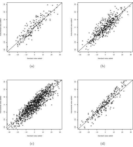
Figure 5: Comparison of the standard value-added versus the value-added cor-rected for endogeneity for (a) Public schools of type I; (b) Public schools of type II; (c) Subsidized schools; (d) Private schools.

(22)

We present results of estimation under HLM5 specification, in whichmat04_ij_andavmat04_j

are considered as endogenous, andfathed _and mothed_{are instrumental variables. Having}

predicted the random effect from this estimation, which we denote by ˆθiv

j , we then compute

a regression on ˆθiv

j to estimate the correction term of the value-added in (4). At this stage,

we note that several options are possible to compute the correction term. In this paper we specify a linear model for the correction term E(θj |mat04ij,avmat04j, XXXij). Because XXXij

contains exogenous variables, we do not include those variables in the linear specification. We thefore estimate the conditional expectation by a linear regression of avmat04_j _{on ˆ}_θiv

j

with school type fixed effects. The estimated coefficients of the regression is ˆ

θiv

j = 46.63 + 5.9δP P −3.9δII−4.2δI−0.17avmat04j+ηj

where δP P, δII, δI are dummy variables for private, type II and type I schools respectively.

All estimated coefficients have p-value less that 0.01.

Figure 5 shows the value-added obtained from (4) versus the value-added obtained from a standard, exogeneous HLM analysis. The Spearman’s rank correlation between the two calculations of the value-added over the whole sample is 0.9. This quantifies the impact of the correction on the ranking of schools. This correlation is similar for each schooltype: it is 0.9 (Public type I schools), 0.86 (Public type II schools), 0.91 (Subsidized schools) and 0.93 (Private schools).

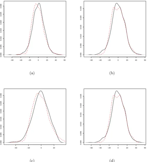
To interpret the change in the calculated value-added it is useful to look at the density of the value-added by type of school. Figure 6(a) superimposes the density of the standard value-added for public schools (type I, dashed line) and subsidized schools (solid line). The same picture after the correction for endogeneity is displayed in Figure 6(b). The gap that appeared in Figure (a) between the mode of the two types of schools is clearly reduced after the correction. The same conclusion is made when comparing the value-added of public schools and private schools (Figures (c) and (d)). It is also worth mentionning that two modes appear in the value-added of public schools after correction for endogeneity. The emergence of differentiated public schools according to their effectiveness is an interesting substantive question for further research.

5 Conclusion

The main message of the paper is the following. In models of value-added, the lagged test score that is included as an explanatory variable is very often endogenous. It is in particular the case when there is little mobility of students between the test occasions. We have shown the impact of this endogeneity on the calculation of the value-added from a linear multilevel model, and we have developed a value-added calculation that is robust to this endogeneity. The paper also raised several questions for further research. We would like to conclude by summarizing three such questions.

1. The value-added under endogeneity is the prediction of the school random effect plus a correction term that we have found to be a conditional expectation, see the above equation (4). In this paper, the correction term is considered as linear but of course

(23)

−60 −40 −20 0 20 40 60 0.000 0.005 0.010 0.015 0.020 0.025 0.030 (a) −60 −40 −20 0 20 40 60 0.000 0.005 0.010 0.015 0.020 0.025 (b) −40 −20 0 20 0.000 0.005 0.010 0.015 0.020 0.025 0.030 (c) −60 −40 −20 0 20 40 60 0.000 0.005 0.010 0.015 0.020 0.025 (d)

Figure 6: Density of the standard value-added (a and c) and density of the value-added corrected for endogeneity (b and d). The dashed, red line is the density for public type I schools. The solid, black line is the density for subsidized schools (a and b) and private schools (c and d).

(24)

other choices might be possible here. A study of the specification of this correction term would be valuable for the generic calculation of the value added under endogene-ity.

2. The paper provides a structural definition of the value-added as a difference between two conditional expetations, see equation (3). When the multilevel regression is used to model the score evolution, it implies that those two conditional expectations are linear. However non linearities of some explanatory variables (including the lagged score) is questionable and might be supported by a nonparametric analysis of the variables in presence. The definition of the value-added given by equation (3) opens the door for a nonlinear analysis of score evolution.

3. A substantive question appeared in our analysis of the value-added under endogeneity for public schools in Chile. As we have shown in Figure 6, the value-added of those schools is bimodal, suggesting the existence of two distinct groups of public schools according to their effectiveness. One mode is even larger than the mode we have found for private or subsidized schools. This result calls for further investigation and characterization of public schools that belong to one or the other mode.

A

Instrumental HLM modelling

For the sake of generality, we denote byYij the contemporaneous score of studentibelonging

to schoolj and byZij the endogenous variables. In our application,Zij contains covariates

depending on the lagged score. We also recall the notationXXXij for the vector of exogeneous

explanatory covariates andθj for the school-specific latent effect. By endogeneity, we mean

that the covariance between θj and Zij is not vanishing. To solve the endogeneity issue,

we suppose to have a vector of instrumental variables, denoted by WWWij. The intuition

behind instruments is that they are correlated to the endogenous variables, but they are not correlated with θj.

We can specify the normal instrumental HLM model as follows: (i) (Yij |Zij, XXXij, WWWij, θj)∼N XXXijβ+γZij+θj, σ2 (ii) (Zij |XXXij, WWWij, θj)∼N XXXijααα+WWWijζζζ+δθj, τ2 (iii) (θj |XXXij, WWWij)∼N 0, µ2 .

Condition (iii) implies that E(θj | XXXij, WWWij) = 0 and, therefore, (Xij,Wij) and θj are

uncorrelated. In other words, bothXXXij andWWWij are exogenous variables with respect toθj.

Condition (i) implies that, conditionally on (Zij, XXXij, θj), the contemporaneous scoreYij is

mutually independent ofWWWij. Thus, if (i) is rewritten as

Yij =XXXijβ+γZij+θj +ǫij, ǫij ∼N(0, σ2),

then E(ǫij | WWWij) = 0. This condition, along with cor(WWWij, θj) = 0, define WWWij as an

instrument. It can be shown that the parameters of the instrumental HLM model are identified provided the dimension of the vector WWWij is at least equal to the number of