8 - 1
Power Low Modified Dual Priority in Hard Real Time Systems with Resource
Requirements
M.Angels Moncusí, Alex Arenas
{amoncusi,aarenas}@etse.urv.es
Dpt d'Enginyeria Informàtica i Matemàtiques
Universitat Rovira i Virgili
Campus Sescelades, Av dels Països Catalans, 26
E-43007 Tarragona, Spain
Jesus Labarta
[email protected]
Dpt d’Arquitectura de Computadors
Universitat Politècnica de Catalunya
Jordi Girona, 1-3. D6 Campus Nord
08034 Barcelona, Spain
Abstract
We present an extension of the Power Low Modified Dual Priority scheduling algorithm that allows hard real time system to use shared resources without compromising the timing constraints of the applications while keeping a low energy consumption. We compare the energy saving of our algorithm with a modification of the Low Power Fixed Priority algorithm that uses shared resources. The results in a Computerized Numerical Control case study shown that the presented algorithm improves LPFPSR energy saving. The total energy saving is closely related to the consumption of the Worst Case Execution Time (WCET), the saving ranges from the 16% of the energy when the 100% of the WCET is consumed, to the 98% of the energy when the 10% of the WCET is consumed.
1.
Introduction
Real time systems are often located in environments where low energy consumption is crucial from the operability and lifelong of the systems point of view. A lot of efforts have been made during the last decade to minimize the power consumption at different levels of the design of real-time systems ranging from semi-conductor level (the logic gate level and the chipset architecture) [1,2] to the operating system and compilation level [3,4,5 and references therein].
The most powerful power aware technique nowadays, consists in to reduce the clock speed along with the voltage supply (Dynamic voltage scaling DVS) or even power down the processor whenever the system does not require its maximum performance [5-8]. At the operating system level, one of the most promising approaches to save energy is the use of scheduling to perform correct DVS, especially when the time constraints of hard real time system must be considered. Taking advantage of the idle time of the processor due to the scheduling of task to reduce the speed has been shown to save significant amounts of energy [5,6,8,9].
Moreover, the scheduling techniques in power saving have been studied in the off-line and on-line scenarios. In the first the scheduling algorithm generates “a priori” a calendar and calculates clock speeds, after that, during run-time the scheduler follows the marked steps [3]. In the
on-line scheduling, the decision of which task executes and the clock speed is run-time determined [8,9].
However, in all these studies the framework usually ignores the specificity of many real time systems that use shared resources. In these systems tasks are not independent since they interact with each other by sharing resources such as data or devices, and the scheduling becomes more complicated. To ensure consistency of these sharing resources, mutual exclusion among competitive tasks must be guaranteed (the piece of code executed under mutual exclusion constraint is called a critical section). When using priority-driven policies to schedule this real-time task sets with shared resources, we must cope with the priority inversion problem [10] that occurs when a high priority task is forced to wait for the execution of lower priority task to preserve mutual exclusion in a resource. This high priority task is blocked until the low priority task releases the mentioned resource. Besides, the determination of the worst blocked time is not straightforward because other tasks could pre-empt the task that holds the resource. So, the priority inversion problem leads to unbounded worst case response time that adversely affects the predictability of the hard real time system.
A mechanism to coordinate the access to shared resources in fixed priority scheduling reducing the priority inversion problem consist in to use protocols that change the priority of the tasks according with the access to shared resources. For example, the Priority Inheritance protocol [10] forces the task that holds the resource to inherit the priority of the higher priority task that wants to allocate the resource. This protocol bounds the worst blocking time, but if a high priority task uses several resources, it can be unfortunately blocked for every resource, this phenomenon is know as chaining blocking. To solve this problem one can use the Priority Ceiling protocol [10], this protocol avoids deadlocks and chained blocking i.e. each instance of each task only can be blocked once during all its execution time. This behavior is obtained by increasing the priority of the current task to the highest priority of the tasks that want to allocate this resource during its lifetime (this priority is defined as the “ceiling” of the resource).
In the present work we embedded the Priority Ceiling protocol [10] in two different scheduling algorithms designed to save energy. We will present a comparison of the results obtained with the Low Power Fixed Priority
Scheduling LPFPS proposed by Shin et al [8] with shared resources versus the Power Low Modified Dual Priority Scheduling [9] with shared resources.
The power efficiency of these two algorithms relies in to run the tasks at the lowest speed that makes possible that the active task and the rest of tasks meet their timing constraints, and power-down the processor when there is a large enough idle interval. This approach is especially interesting because the quadratic dependency of the power dissipation, in CMOS circuits, on the voltage supply [1]. The power dissipation satisfies approximately the formula
clk dd L t
C
V
f
p
P
≅
2where pt is the probability of switching in power transition,
CL is the loading capacitance, Vdd the voltage supply and fclk
the clock frequency. That means that it is always energetically favorable to perform slowly and at low voltage than quickly at high voltage.
The rest of this paper is organized as follows, in the next section we describe the framework and the basic ideas of the Priority Ceiling protocol. Section 3 is devoted to the modification of the algorithm to use shared resources reducing the energy consumption. Finally, in section 4 we present the experimental results and the comparison with Low Power Fixed Priority scheduling with Priority Ceiling protocol, and finally in section 5 we draw the conclusions.
2.
Framework and Priority Ceiling protocol
The general framework of the hard real-time system we are going to deal with is made up of periodic tasks1. These tasks — numbered 1 ≤ i ≤ n — are specified by their periods, worst case execution times and deadlines (Ti, Ci
and Di respectively). The use of shared resources implies
that the tasks have critical sections that could be simulated by atomic subtasks. Following this line, these periodic tasks are divided conceptually pre-run time into subtasks — numbered 1 ≤ j ≤ s — with the same period Ti and deadline
Di that the periodic task, but different worst case execution
time Cij assuring that ΣCij = Ci. Some of these subtasks can
use shared resources during all their execution time. Note that the proposed partition in subtasks of the real tasks is performed only at the logical level of abstraction to deal with the present problem theoretically, this partition has no implications at the physical level of the implementation. Once the problem will be conceptually solved the implementation of the algorithms will work perfectly without affecting the structure of the real tasks.
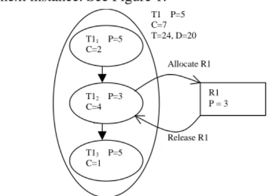
The decomposition of every task in subtasks has been performed as follows: suppose that we have a task T1 with a period T=24 units and a deadline D=20 units, a worst case execution time of 7 units and a priority P=5 (the lower the number, the higher priority). We assume the execution of the worst case execution time and, that task T1, needs to access a shared resource R1 during 4 time units after
1 The results are not exclusive for periodic tasks. We have considered only
periodic tasks as a matter of simplicity.
executing 2 time units and then releases the resource until the next instance. See Figure 1.
Allocate R1 Release R1 T1 P=5 C=7 T=24, D=20 T11 P=5 C=2 T12 P=3 C=4 T13 P=5 C=1 R1 P = 3
Figure 1: Example of the division of one task into subtasks.
Task T1 will be conceptually divided into three subtasks with the following characterization: same period and deadline as task T1. The first subtask T11 will have a
WCET of 2 that corresponds to the execution time before allocating the resource. T12 will have a WCET equal to 4,
the execution time inside the resource (critical section) and finally the third subtask T13 will have a WCET of 1, that
corresponds to the rest of execution time outside the resource. To ensure the causal precedence, as soon as T11
finishes it sends a message to provoke the initiation of T12.
Once T12 allocates the resource R1 increases its priority to
the priority of this resource (we will see later how it is determined), it executes, it releases the resource, and it sends a message to provoke the initiation of T13 and finish.
At this moment T13 starts to execute normally. This process
has been reproduced for every task in the task set. We assume that the messages are instantaneous for the sake of simplicity.
The computation times for context switching and for the scheduler are assumed to be negligible, this enables us to perform the analysis straightforward without danger of loosing generality. The extent to which these assumptions are realistic is discussed in the analysis of the algorithm given in [7], and it turns out to be practical if the switch is subsumed to the worst case execution times of the different tasks.
The whole system is organized as concurrent tasks ruled by a pre-emptive static priority-based scheduler. This static priority can be violated when two tasks want to access a shared resource, a lower priority task may block a higher priority task if it succeeds to access to the shared resource earlier (priority inversion). This problem can be avoided applying the Priority Ceiling protocol [10]. The Priority Ceiling protocol modifies the calculation of the worst case response time (WCRT) accounting for the possible blocking caused by low priority tasks to higher priority tasks.
To apply the Priority Ceiling protocol, we proceed calculating first the “ceiling” of each resource as the priority of the highest priority task that can access this resource. The worst case blocking time that a task i can experiment due to the Priority Ceiling protocol is determined by the longest critical section of the lower
8 - 3 priority task accessing to shared resources with ceilings
equal or higher than the priority of task i [10].
The schedulability of the system can be tested off-line using the iterative technique proposed by Joseph and Pandya [11] and later extended by Audsley et al. in [12] to deal with shared resources. It compares the different WCRT obtained summing all the possible blocking contributions of the tasks that could preempt task i assuming an initial WCRT=0. The iteration n+1 is computed as follows,
j ) i ( hp j j n i i i 1 n i T *C WCRT C B WCRT
∑
∈ + + + =where Bi is the longest blocking time due to lower priority
tasks and hp(i) is the set of task that could preempt task i, i.e all tasks with higher priority than task i The iterative process starts with WCRTi
0
=0 and it stops when WCRTi n+1
= WCRTi n
or when WCRTi n+1
> Di , in this latter case the
system is not schedulable.
We can apply this formula straightforward to our framework because the scheduler assures that the precedent subtask finishes before the next subtask starts. The period, deadline and priority of the subtasks of one task are the same.
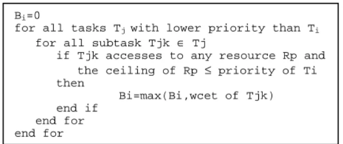
The calculation of the longest blocking time (Bi) for a
task Ti , based on [10], is shown in Figure 2.
Figure 2. Determination of the longest blocking time
3.
Power Low Modified Dual Priority with
Shared Resources
Here we extend the Power Low Modified Dual Priority Scheduling algorithm (based on the Dual Priority scheduling [13]) to deal with shared resources in a hard real-time system. The original Power Low Dual Priority Scheduling algorithm guarantees to meet the temporal constraints and significant energy consumption reduction by slowing speed and voltage jointly (assuming a linear relation between speed and voltage supply decreasing). To extend this behavior to real time systems with shared resources, we need first to solve the problem of priority inversion, because it can cause our algorithm to find false schedulability situations. Our new approach determines when and how to apply the Priority Ceiling protocol in PLMDPR to avoid the priority inversion problem.
The main idea is to apply the same algorithmic scheme presented in PLMDP, but dealing with subtasks directly instead of with the whole tasks, in this way it is possible to reassign priorities according to the Priority Ceiling protocol when necessary.
Initially, we have fixed priorities assigned to tasks according to a fixed priority criterion. At this moment, all subtask of the same task have the priority of the task.
The scheduler modifies the priority of a subtask when it accesses to a shared resource, specifically the scheduler applies the Priority Ceiling protocol increasing the priority of the subtask to the ceiling of the resource this subtask accesses. The PLMDPR defines two levels of priorities that are organized as follows, the highest level, or upper run queue (URQ) is for tasks that can no longer be delayed by less priority tasks otherwise they will miss their deadlines. The second level, or lower run queue (LRQ) is occupied by those periodic tasks whose execution time can still be delayed without compromising the meeting of their deadlines. The ceiling of the resource in this scheme corresponds to the priority in the URQ of the highest priority task that could gain access to this resource.
The scheduling algorithm is driven by the following events:
1. Activation of some periodic task. In this case this task is queued to the LRQ sorted by its promotion time instant. At this moment this task can pre-empt a lower priority task currently in execution.
2. Promotion time instant of some task (this time is explicitly calculated in [9]). In this case, this task is promoted from the LRQ to the URQ, and at this moment the task can pre-empt a lower priority task currently in execution.
3. Allocation of a shared resource. The executing subtask increases its priority to the ceiling of this resource. After allocation of the resource pre-emption by a higher priority task can occur.
4. Release of a shared resource. The subtask decreases its priority to the priority of the task. At this moment this task can be pre-empted by a higher priority task. Finally, when a task finishes its execution, the next executing task is selected by picking the highest priority task from the highest non-empty priority levels (i.e. URQ or LRQ, in this order).
Once the scheduler decides which task to execute, before start the execution it needs to fix the ratio of processor speed according with the maximum spreading in time we are allowed. The speed ratio is calculated following the heuristics proposed by Shin et al. [8] that is built on the assumption that the delay for the reduction is negligible. The safeness of the system under these conditions is proved on theorem 1 of the cited work. The speed of the processor is determined as follows:
1. If there is not any task in the system, then we set the timer to the next arriving task minus the wake up delay, and power down the processor.
2. If there is more than one task in the URQ then it has to be executed at maximum speed.
3. If there is only one task in the URQ then it can be executed at low speed where the speed ratio is:
Bi=0
for all tasks Tj with lower priority than Ti for all subtask Tjk ∈ Tj
if Tjk accesses to any resource Rp and the ceiling of Rp ≤ priority of Ti then
Bi=max(Bi,wcet of Tjk) end if
end for end for
tc ) td , tp ( min )) C ( remainig , tc tp min( ratio Speed i k i k − − =
where tpk is the promotion time instant of any task in
the system excluding the current executing task, Ci is
the worst execution time of the current executing task, tdi is the deadline of the current executing task, and
finally tc is the current time.
4. If there are not any task in the URQ but there are some tasks in the LRQ then we can execute at low speed where the speed ratio is calculate as follows:
At practice only certain discrete values of the frequency of the clock, and then speed, are attainable depending on the accuracy of the tuning, in this case the frequency selected should be a frequency equal or larger than the frequency obtained by the calculations to ensure time constraints. A comprehensive example of the functioning of the algorithm in a toy model is presented in the appendix, in this example we can observe the effects of coarse or fine graining of the speed of the processor.
4.
Results and discussion
In this section we present the comparison results of the Low Power Fixed Priority scheduling with shared resources using Priority Ceiling (LPFPSR) versus the Power Low Modified Dual Priority scheduling with shared resources (PLMDPR).
LPFPSR is based on a fixed pre-emptive priority scheduling with power awareness. This algorithm consists on executing tasks as slow as possible while satisfying time constraints. LPFPSR reduces clock speed along with voltage supply when there is a unique task ready to execute, otherwise the scheduling does not guarantee the time constraints of the rest of tasks of system. It also powers down the processor when there are not ready tasks. The differences between LPFPS and the PLMDP are studied in [9].
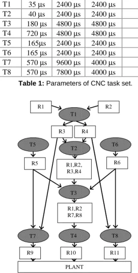
To check the capabilities of both algorithms, we have simulated several situations of a Computerized Numerical Control (CNC) task set [14], this example represent a typical benchmark of multi-tasking system sharing data in many interacting and overlapping data paths. We compare the total energy consumption results (per hyper-period) obtained. In Figure 3 we present the task graph of this system just to show the complexity of the real-time application. In this figure the oval objects represent tasks
and the rectangular objects correspond to data items (shared resources). The characteristics (Worst Case Execution Time, Period, Deadline and the priority) of the task set is shown in the Table 1.
We investigate different configurations related to the way in which the different tasks allocate and release resources. We have placed the non-critical section of the task execution, which in our approach is represented as a subtask (ncs), in three different positions along the execution process. We assume that the tasks allocate the resource (or critical section, cs) at the beginning of the execution (cs-ncs), before termination (ncs-cs), or in the middle of the execution process (cs-ncs-cs). With these three different situations we obtain trends for the most general situation were the critical section could appear anywhere, and several times, during the execution process.
Task WCET Period Deadline Priority T1 35 µs 2400 µs 2400 µs 1 T2 40 µs 2400 µs 2400 µs 2 T3 180 µs 4800 µs 4800 µs 3 T4 720 µs 4800 µs 4800 µs 4 T5 165µs 2400 µs 2400 µs 5 T6 165 µs 2400 µs 2400 µs 6 T7 570 µs 9600 µs 4000 µs 7 T8 570 µs 7800 µs 4000 µs 8
Table 1: Parameters of CNC task set.
Figure 3: Task graph of the CNC control system.
The time a task is executing the critical section, i.e. it is inside the shared resource is represented as a percentage of the total execution time of the task. We vary this time from 0% to 100% of the worst case execution time of the task to have a wide evaluation of performance.
The results of all the experiments are represented in terms of the normalized average energy consumption. The light gray column represents the results of the LPFPSR and
if tak < tpi and tpk < tpi then speed minimum -tc ta 1 Speed k− =
else if tph< tpl+Ci then -- h∈hp(i), l∈lp(i)
tc ) td , tp ( min )) C ( remaining , tp tp min( Speed i h i i h − − = else tc ) td , C tp ( min )) C ( remaining , tp C tp min( Speed i i l i i i l − + − + = endif endif T1 T2 T3 T4 T5 T6 T8 T7 R1 R2 R5 R6 R1,R2 R7,R8 R9 R10 R11 R1,R2, R3,R4 R3 R4 PLANT
8 - 5 the dark gray column represents the results of the
PLMDPR. The simulation covers one hyper-period (that is, the minimum common multiple of the tasks periods).
In Figures 4 to 6, we show the behavior of both algorithms when the time the tasks execute inside the shared resources varies from 0% to 100%. In figure 4, the tasks exhaust the 100% of the WCET, 60% in figure 5 and 20 % in figure 6. The average factor of improvement of our algorithm in front of LPFPSR is 15 % if all tasks use the 100% WCET, 48% if all tasks use the 60% of the WCET and 75% if all tasks use the 20% of the WCET.
0 0,2 0,4 0,6 0,8 1 % of shared resources N o rm a liz e d e n e rg y c o n s u m p ti o n L PFPS PL MDP
Figure 4: Normalized energy consumption varying the time
inside the resource when the 100% of WCET is exhausted
0 0,2 0,4 0,6 0,8 1 % of shared resources N o rm a li z e d e n e rg y c o n s u m p ti o n L PFPS PL MDP
Figure 5: Normalized energy consumption varying the time
inside the resource when the 60% of WCET is exhausted.
0 0,2 0,4 0,6 0,8 1 % of shared resources N o rm a li z e d e n e rg y c o n s u m p ti o n L PFPS PL MDP
Figure 6: Normalized energy consumption varying the time
inside the resource when the 20% of WCET is exhausted.
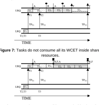
In all these figures, we observe a significant decreasing of the energy consumption in both algorithms when the 100% of the execution time of all tasks is exhausted inside the shared resources. Here we present the analysis of this particular situation. See Figures 7 and 8.
Let us assume that we have three tasks: T1, T2 and T3. The priority of the tasks are T1=3, T2=2 and T3=1 (the smaller the numbers the higher the priorities). T1 and T2 both access to the same resource R1, so the ceiling of R1 will be the priority of T2. The promotion time of T1 is
smaller than the promotion time of T2 and this is smaller than the promotion time of T3, then, in the LRQ, the order was T1, T2 and T3.
Figure 7:Tasks do not consume all its WCET inside shared
resources.
Figure 8: Tasks consume all its WCET inside shared
resources.
In Figure 7, initially, the task T1 is executing in the LRQ, at promotion time TPT1, task T1 promotes to the
URQ and continues it execution. At promotion time TPT2,
task T2 promotes to the URQ. As T1 has allocated the resource its priority is the ceiling priority of the resource (that is the same as T2). T2 could not pre-empt, and it must wait until T1 releases the resource and returns to its priority base. Now T2 can pre-empt the CPU and it executes. As there are two tasks in the URQ the processor speed could not be reduced. After T2 finishes there is only one task in the URQ and the speed can be reduced, but the remaining execution time is small. In Figure 8, as soon as T1 release the resource, it finishes, so T2 can execute at low speed during all its execution. This latter situation is energetically favorable, i.e. the ratio time/speed is larger.
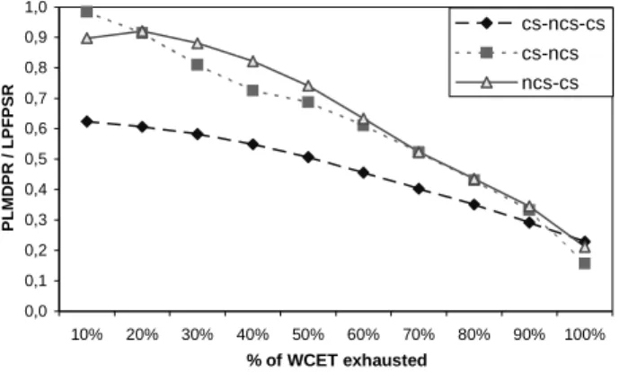
Finally, in Figure 9, we represent the total energy saving in the three possible configurations when the task consumes different ranges of its WCET from 10% to 100%. Each point in the graph represents the ratio of the accumulated energy saving varying the percentage of the WCET exhausted in the shared resources from 0% to 100%. We observe that in the cs-ncs-cs case, where the Bi caused by
the resource is the half value of the Bi of the cs-ncs and the
ncs-cs, and it occurs twice, the PLMDPR algorithm improves LPFPSR between a 23% and a 62%. On the case cs-ncs the improvement of the PLMDPR varies between 16% and 98%, and finally in the case ncs-cs the improvement varies from 21% to 90%. The reason of the difference behavior between cs-ncs-cs and cs-ncs or ncs-cs, is that in the former the pre-emption can occur when a task has still not finished and another task, that pre-empts the executing task, comes to the URQ forcing the scheduler to increase the speed of the processor to the maximum value.
A R T2 URQ T12 T21 TPT2 T2,T3 T13 T1 T11 LRQ A R T22 T23 TPT3 TPT1 T3 TIME T11 F F A T2 URQ T12 T13 TPT2 T2,T3 T23 T1 T11 LRQ R,F,A T21 T22 TPT3 TPT1 T3 TIME T11 R,F
However, when there is a unique critical section, the algorithms perform equivalently in both configurations (cs-ncs) and (ncs-cs). 0,0 0,1 0,2 0,3 0,4 0,5 0,6 0,7 0,8 0,9 1,0 10% 20% 30% 40% 50% 60% 70% 80% 90% 100% % of WCET exhausted P L M D P R / L P F P S R cs-ncs-cs cs-ncs ncs-cs
Figure 9: Energy consumption ratio PLMDPR/LPFPSR in
function of the time inside the resource for three different configurations of the access to the shared resources.
5.
Conclusions
We have presented an extension of the Power Low Modified Dual Priority scheduling algorithm that allows hard real time system to use shared resources without compromising the timing constraints of the applications while keeping a low energy consumption. This approach has been shown to over-perform the LPFPSR power saving by an average factor, in the case of a Computerized Numerical Control task set, that range from 16% up to 98% depending on the use of sharing resources and the consumption of the worst case execution time that does the application. The algorithm does not increase the complexity of the LPFPSR and can be implemented in most of the kernels.
6.
References
[1] A.P. Chandrakasan, S. Sheng and R. W. Brodersen, “Low-power CMOS digital design”, IEEE Journal of Solid-State
circuits, vol. 27, pp. 473-484, April 1992.
[2] J. Rabaey and M Pedram (Editors). "Low Power Design Methodologies". Kluwer Academic Publishers, Norwell, May, 1996.
[3] S.T. Cheng, S.M. Chen and J.W. Hwang, "Low-Power Design for Real-Time Systems", Real-Time Systems,15, pp 131-148, 1998.
[4] D. Mosse, H. Aydin, B. Childers and R. Melhem, “Compiler-assisted power-aware scheduling for real-time applications”
Workshop on Compilers and Operating systems for Low Power COLP 2000, Chateau Lake Louise, Banff, Canada, October 2000.
[5] P. Pillai and K.G. Shin, “Real-time dynamic voltage scaling for low-power embedded operating systems” 18th ACM
Symposium on Operating Systems Principles, Philadelphia,
Pennsylvania, October 2001.
[6] Transmeta Corporation, Crusoe Processor Specification, http://www.transmeta.com
[7] H. Aydin, R. Melhem, D. Mosse and P. Mejia-Alvarez, “Determining optimal processor speeds for periodic real-time tasks with different power characteristics” 13th Euromicro
Conference on Real-Time Systems, Delft, Netherlands, June 2001.
[8] Y. Shin and K. Choi, “Power conscious Fixed Priority scheduling in hard real-time systems” DAC 99, New Orleans, Louisiana, ACM 1-58113-7/99/06, 1999.
[9] M.A. Moncusí, A. Arenas and J. Labarta, "Improving Energy Saving in Hard Real Time Systems via a Modified Dual Priority Scheduling", ACM SigArch Computer Architecture Newsletter, Vol 29, No.5, pp 19-24, December 01.
[10] L. Sha, R. Rajkumar and J.P. Lehoczky. "Priority Inheritance Protocols: An approach to Real-Time Synchronization", IEEE
Transactions on Computers, Vol 39, No 9, pp 1175-1185,
September 90
[11] M.Joseph and P.Pandya. "Finding response times in a real-time system”, The Computer Journal, vol 29, no 5 pp 390-395, October 86.
[12] N.Audsley, A. Burns, M.Richardson, K. Tindell and A.J. Wellings. "Applying new scheduling theory to static priority pre-emptive scheduling", Software Engineering Journal, pp 284-292, September 93.
[13] R. Davis and A.J. Wellings, "Dual Priority scheduling",
Proceeding IEEE Real Time Systems Symposium, pp. 100-109,
December 1995.
[14] N. Kim, M. Ryu, S. Hong, M. Saksena, C. Choi and H. Shin, "Visual assessment of a real-time system design: a case study on a CNC controller", Proceedings IEEE Real-Time Systems
symposium, December 1996.
Appendix
We present a toy model example to enlighten the functioning of the algorithms in the two main aspects i.e. the speed reduction and allocation and release of shared resources. The proposed task model is presented in Table 2. Name Period Deadline WCET Share resource
T1 50 50 10 X
T2 80 80 20
T3 100 100 40 X
Table 2 Parameters of a toy model example.
T1 T1 T1 T1 T2 T3 T2 T2 T3 T1 T2 T1 T3 T1 T2 T1 T3 1 0.75 0.50 0.25 0 200 250 300 350 400 0 50 100 150 200 1 0.75 0.50 0.25 0 T1 T2 T3 T1 T2 T3 sp e e d sp ee d time time X X
The task is inside the resource
X X X X X X X X X X X
X X X X X
X X X X X X X
Figure 10: LPFPSR when tasks consume the 100% of the
8 - 7 Consider Figure 10 that represents the behavior of the
LPFPSR when the tasks consume the 100% of the WCET. The speed reduction can not be performed until t=160, when there is only task T2 at the system. We reduce the
speed until the arrival of T1 and T3 to the system again at
t=200. Essentially the same occurs at t=260 and t=360. The resource allocation works as follows: at t=50 T1 tries to
allocate the resource but T3 is inside and must wait until it
releases the resource. At t=240 T2 arrives with a higher
priority than T3, but using the priority ceiling protocol (the
ceiling is the priority of T1) T3 inherits the priority of the
ceiling so T2 can not preempt T3.
The energy consumption depends on the graining of the speed reduction as follows: considering 10 speed fractions the energy consumption is 287.5 units, considering 100 speed fractions the energy consumption is the same 287.5 units. 1 0.75 0.50 0.25 0 T1 T1 T1 T1 T2 T3 T2 T2 T3 T1 T2 T1 T3 T1 T2 T1 T3 1 0.75 0.50 0.25 0 200 250 300 350 400 0 50 100 150 200 T1 T2 T3 T1 T2 T3 sp ee d sp ee d time time X X
The task is inside the resource
X X X X X X X X X X X
X X XX X
X X X X X X X
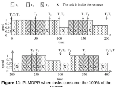
Figure 11: PLMDPR when tasks consume the 100% of the
WCET
In Figure 11 we represent the behavior of the PLMDPR when the tasks consume the 100% of the WCET. Let us see the speed reductions. This time, T1 and T2 promote to the
URQ as they arrive to the system. T3 promotes 20 tim e
units after their arrival. At t=100, we can reduce speed because the only task at the URQ is T1 and T3 is at the
LRQ. After promotion of T3 at t=120 something interesting
happens. In principle, the speed could be reduced but, due to that fact that at t=150 T1 will promote again, the idle time
is shorter than the time T3 needs to finish its execution and
then the speed is not reduced. The same scenario occurs at t=200 and t=300.
On the other hand, the resource allocation works identically to the LPFPSR case.
The energy consumption depends on the graining of the speed reduction as follows: considering 10 speed fractions the energy consumption is 278.72 units, considering 100 speed fractions the energy consumption is 277.03 units.
Figure 12 represents the behavior of the LPFPSR when the tasks consume the 50% of the WCET. At t=15, T3 is the
only task in the system, however we can not reduce the speed because it needs 40 time units, in the worst case, to execute and T1 will arrive at t=50. At practice it executes
only during 20 time units and the rest 15 units the system is free. The rest of reductions are straightforward.
T1 T1 T1 T1 T2 T3 T2 T2 T3 T1 T2 T1 T3 T1 T2 T1 T3 1 0.75 0.50 0.25 0 200 250 300 350 400 0 50 100 150 200 1 0.75 0.50 0.25 0 T1 T2 T3 T1 T2 T3 sp e ed sp ee d time time X X
The task is inside the resource
X X X X X X X X X X X X X X X
Figure 12: LPFPSR when tasks consume the 50% of the
WCET
The priority ceiling in this example implies that T2 must
wait due to the priority ceiling protocol at t=320.
The energy consumption depends on the graining of the speed reduction as follows: considering 10 speed fractions the energy consumption is 136.35 units, considering 100 speed fractions the energy consumption is 135.74 units.
1 0.75 0.50 0.25 0 T1 T1 T1 T1 T2 T3 T2 T2 T3 T1 T2 T1 T3 T1 T2 T1 T3 1 0.75 0.50 0.25 0 200 250 300 350 400 0 50 100 150 200 T1 T2 T3 T1 T2 T3 sp ee d sp ee d time time X X
The task is inside the resource
X X X X X X X
X X X X X X X
X X
Figure 13: PLMDPR when tasks consume the 50% of the
WCET
In Figure 13 we represent the behavior of the PLMDPR when the tasks consume the 50% of the WCET. In this case the speed reduction take advantage of the idle time
The speed reduction occurs before the promotion of T3 at
t=20. At t=50 T1 is the only task at the system and the speed
can be reduced again.
At t=100 T1 can reduce the speed until T3 promotes at
t=120, that can reduce the speed again until t=150.
The energy consumption depends on the graining of the speed reduction as follows: considering 10 speed fractions the energy consumption is 104.21 units, considering 100 speed fractions the energy consumption is 99.57 units.