Pseudo-likelihood estimation of multidimensional polytomous item response theory models

PSEUDO-LIKELIHOOD ESTIMATION OF MULTIDIMENSIONAL POLYTOMOUS ITEM RESPONSE THEORY MODELS

BY

YOUNGSHIL PAEK

DISSERTATION

Submitted in partial fulfillment of the requirements

for the degree of Doctor of Philosophy in Educational Psychology in the Graduate College of the

University of Illinois at Urbana-Champaign, 2016

Urbana, Illinois

Doctoral Committee:

Professor Carolyn J. Anderson, Chair Professor Jeffrey A. Douglas

Associate Professor Jinming Zhang Assistant Professor Steven Culpepper

ii Abstract

Log-multiplicative association (LMA) models, special cases of log-linear models, can be used as multidimensional item response theory (MIRT) models for polytomous items (Anderson, Verkuilen and Peyton, 2010; Anderson, 2013). LMA models do not require numerical

integration for their estimation nor do they require assumptions regarding the marginal

distribution of the latent variables. However, maximum likelihood estimation (MLE) of LMA models requires iteratively computing fitted values for all possible response patterns. Standard estimation methods for large numbers of items fail because the number of possible response patterns increases exponentially as the number of items and response options per item increase. In this study, a new algorithm is proposed to solve this estimation problem.

Anderson, Li and Vermunt (2007) proposed using pseudo-likelihood estimation (PLE); however, their solution only applies to models in the Rasch family, which exploits the

relationship between log-linear and logistic regression models. Their method is extended to more general models by adding an additional step that estimates slope (item discrimination) parameters for the latent variables.

The new algorithm has two basic steps and simplifies for special cases. In Step 1, a (multinomial) logistic regression model is fit by MLE to one item using rest-scores as an explanatory variable to get new estimates of item slopes that are used in the rest-score for the next item. This process is repeated for each item until all item slopes have been up-dated. Step 2 involves fitting a single conditional logistic regression model for a data set formed by stacking the conditional logistic regressions for each item. This yields new estimates of location (item

iii

difficulty) parameters and the covariance matrix for the latent variables. Steps 1 and 2 are repeated until all parameter estimates converge.

The results of simulation and empirical studies with real data show that the proposed algorithm successfully estimates parameters in more general LMA models with both location and slope parameters as MIRT models.

iv To My Parents

v

Acknowledgments

I would like to express my deepest gratitude to my academic advisor Dr. Carolyn J. Anderson. Dr. Anderson has always been an admirable and brilliant mentor to me, has shown substantial support for my study and work with her inspiration and encouragement, and has strengthened my determination in pursuit of my dream. Her persistent efforts and patience have assisted me overcome many crisis situations and finish this dissertation.

I also wish to give my sincere appreciation to the members of my dissertation committee, Dr. Jeffrey A. Douglas, Dr. Jinming Zhang, and Dr. Steven Culpepper for their constructive comments and insightful suggestions to help me improve my dissertation. I am honored to have each of them on my committee.

I am also grateful to my dear friends, Jin-hee, Jong-ok, Jeong-rae, Sung-sook, Eun-young, and Yeonsook. Their support, care, and encouragement that warms my heart helped me overcome setbacks and stay focused on my graduate study. I greatly value their friendship and I deeply appreciate their belief in me. They are not only my friends but also my sisters.

Most importantly, none of this would have been possible without the love and patience of my family. My parents to whom this dissertation is dedicated to, have been a constant source of love, concern, support, and strength all these years. I would like to express my heart-felt

gratitude to my supportive brothers and their families. Finally, I am deeply thankful to my husband, Taeho and my wonderful sons, Wonwoo and Junwoo, who have stayed with me throughout this journey. I couldn’t have made it without their constant love, dedication, and positive energy.

vi

Table of Contents

List of Tables ... viii

List of Figures ... x

Chapter 1. Introduction ... 1

Estimation of MIRT Models for Polytomous Items ... 1

Estimation of LMA Models as MIRT Models ... 3

Pseudo-likelihood Estimation for LMA Models and Its Limitation ... 5

Research Objectives ... 6

Chapter 2. LMA Models as Multidimensional Item Response Theory (MIRT) Models ... 8

Multidimensional Item Response Models for Polytomous Items ... 8

Multidimensional Compensatory IRT Model for Nominal Responses ... 9

Log-Multiplicative Models (LMA) as Item Response Models ... 11

Chapter 3. Estimation of LMA Models... 25

Maximum Likelihood Estimation (MLE) ... 25

Pseudo-likelihood Estimation (PLE) ... 27

Chapter 4. Proposed Algorithm for LMA Models ... 35

An Overview of the New Algorithm ... 35

Step 1: Conditional Multinomial Logit Models for Each Item ... 36

Step 2: A Stacked Conditional Logistic Regression Model ... 38

The Extended Application of PLE to LMA Models as MIRT Models ... 41

Implementation of PLE in SAS for More General LMA Models ... 42

Chapter 5. Research Methodology ... 47

Simulation Studies for Unidimensional Models ... 47

Simulation Studies for Multidimensional Models ... 49

Evaluation Criteria ... 50

Estimation of Standard Errors of PL Estimates ... 51

Chapter 6. Simulation Studies ... 56

Unidimensional Models with Small Numbers of Items ... 56

vii

Multidimensional Models with Small Numbers of Items ... 85

Multidimensional Models with Large Numbers of Items ... 103

Estimation of Standard Errors of Pseudo-Likelihood Estimates ... 118

Computational Time of PLE for Large Numbers of Items ... 127

Chapter 7. Empirical Studies ... 132

Unidimensional Models with Bullying Items ... 132

Multidimensional Models with Bullying and Victimization Items ... 139

Chapter 8. Discussion and Conclusions ... 144

Estimation of Slope Parameters by PLE ... 144

Comparison of PLE with MLE ... 146

Performance and Estimation Time of PLE for Large Numbers of Items ... 147

Future Direction ... 151

References ... 154

viii List of Tables

Table Page

1 Design matrix for one person for PLE of LMA Rasch model:

Polytomous items with one latent variable ... 33

2 Definitions of the weighted rest-score for item 1 in each step ... 39

3 LMA models as MIRT models covered by the algorithm ... 41

4 An example of ‘Responses’ dataset from six 3-category items ... 43

5 An example of ‘Items” dataset from six items ... 43

6 Example of ‘ItemTraitAdj’ datasets from six items ... 43

7 Example of ‘TraitAdj’ datasets for uni- and multidimensional models ... 44

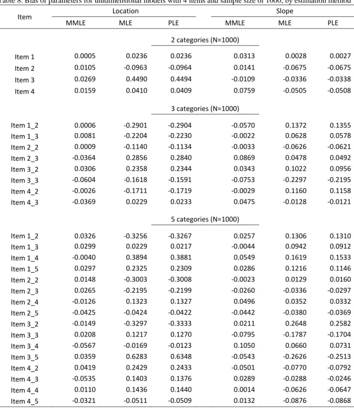
8 Bias of parameters for unidimensional models with 4 items and sample size of 1000, by estimation method ... 57

9 Mean bias, RMSE and their (SDs) and correlation coefficients for location parameters of unidimensional models with 4 and 6 items, by estimation method ... 58

10 Mean bias, RMSE and their (SDs) and correlation coefficients for slope parameters of unidimensional models with 4 and 6 items, by estimation method ... 59

11 Correlation coefficients (r) between the parameter estimates obtained from MLE and PLE for unidimensional models with 4 and 6 items ... 61

12 Mean RMSDiff of parameter estimates between MLE and PLE for unidimensional models with 4 and 6 items. ... 62

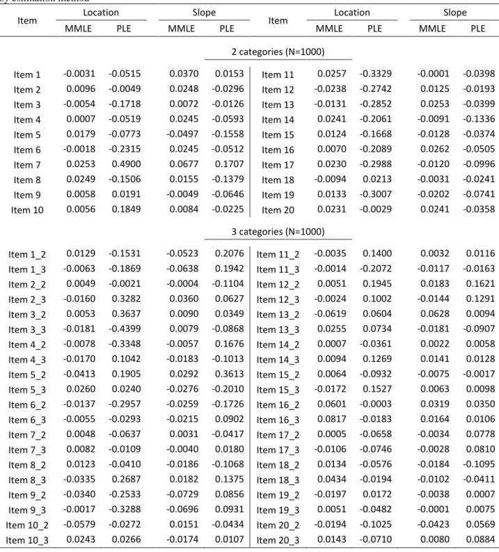
13 Bias of parameters for unidimensional models with 20 items, 2 and 3 categories, and sample size of 1000, by estimation method ... 74

ix

14 Mean bias, RMSE and their (SDs) and correlation coefficients for location parameters of unidimensional models with 20 and 50 items ... 75

15 Mean bias, RMSE and their (SDs) and correlation coefficients for slope parameters of unidimensional models with 20 and 50 items ... 81

16 Bias of parameters for two-dimensional models with 6 items and sample size of 1000, by estimation method ... 88

17 Mean bias, RMSE and their (SDs) and correlation coefficients for location parameters of 2 dimensional models with 4 and 6 items ... 89

18 Mean bias, RMSE and their (SDs) and correlation coefficients for slope parameters of 2 dimensional models with 4 and 6 items ... 90

19 Mean bias, RMSE and their (SDs) and correlation coefficients for location and slope parameters of 3 dimensional models with 6 items ... 96

20 Correlation coefficients (r) between the parameter estimates obtained from MLE and PLE for multidimensional models with 4 and 6 items ... 102

21 Mean RMSDiff of parameter estimates between MLE and PLE for multidimensional models with 4 and 6 items. ... 102

22 Bias of parameters for two- and three-dimensional models with 20 items, 2 and 3 categories and sample size of 1000 ... 104

23 Mean bias, RMSE and their (SDs) and correlation coefficients of PLE for location parameters of multidimensional models with 20 and 50 items ... 106

24 Mean bias, RMSE and their (SDs) and correlation coefficients of PLE for slope parameters of multidimensional models with 20 and 50 items ... 112

x

List of Figures

Figure Page

1 Graphs for (A) one latent variable and (B) two correlated latent variables with four items ... 16

2 LMA Rasch model with I polytomous items and one latent variable... 30

3 The proposed algorithm ... 36

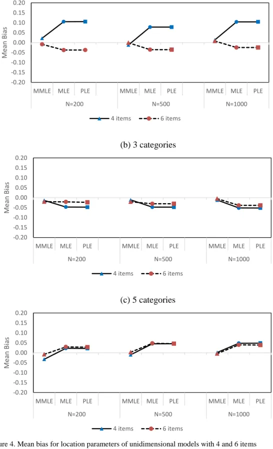
4 Mean bias for location parameters of unidimensional models with 4 and 6 items ... 64

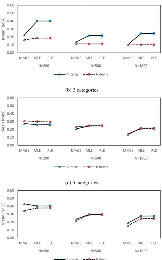
5 Mean RMSE for location parameters of unidimensional models with 4 and 6 items ... 65

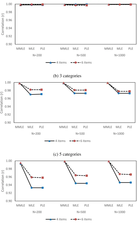
6 Correlation coefficients (r) for location parameters of

unidimensional models with 4 and 6 items ... 67

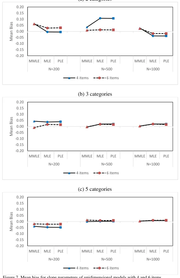
7 Mean bias for slope parameters of unidimensional models with 4 and 6 items ... 69

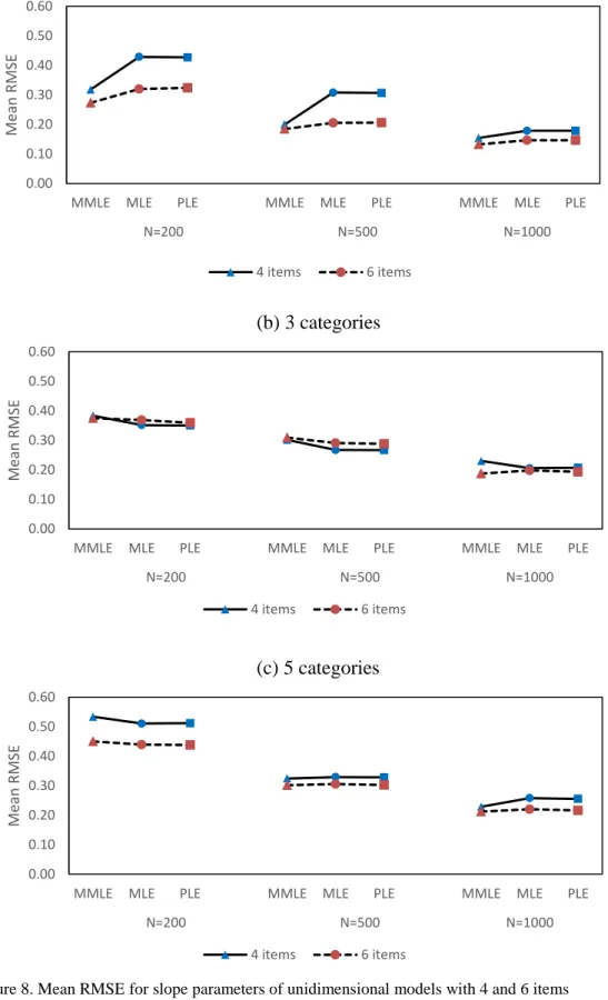
8 Mean RMSE for slope parameters of unidimensional models with 4 and 6 items ... 70

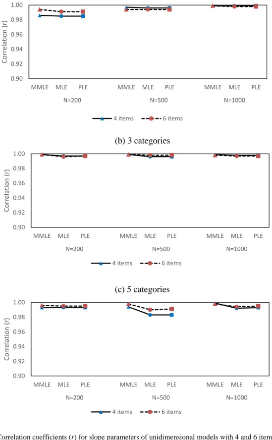
9 Correlation coefficients (r) for slope parameters of

unidimensional models with 4 and 6 items ... 72

10 Mean bias for location parameters of unidimensional models with 20 and 50 items ... 76

11 Mean RMSE for location parameters of unidimensional models with 20 and 50 items ... 78

12 Correlation coefficients (r) for location parameters of

unidimensional models with 20 and 50 items ... 80

13 Mean bias for slope parameters of unidimensional models with 20 and 50 items ... 83

14 Mean RMSE for slope parameters of unidimensional models with 20 and 50 items ... 84

xi

15 Correlation coefficients (r) for slope parameters of

unidimensional models with 20 and 50 items ... 86

16 Mean bias for location and slope parameters of 2-dimensional models with 4 and 6 items... 92

17 Mean RMSE for location and slope parameters of 2-dimensional models with 4 and 6 items... 93

18 Correlation coefficients (r) for location and slope parameters of 2-dimensional models with 4 & 6 items ... 95

19 Mean bias for location and slope parameters of 3-dimensional models with 6 items ... 98

20 Mean RMSE for location and slope parameters of 3-dimensional models with 6 items ... 99

21 Correlation coefficients (r) for location and slope parameters of 3-dimensional models with 6 items ... 101

22 Mean bias of PLE for location parameters of

multidimensional models with 20 and 50 items ... 108

23 Mean RMSE of PLE for location parameters of

multidimensional models with 20 and 50 items ... 109

24 Correlation coefficients (r) of PLE for location parameters of

multidimensional models with 20 and 50 items ... 111

25 Mean bias of PLE for slope parameters of

multidimensional models with 20 and 50 items ... 114

26 Mean RMSE of PLE for slope parameters of

multidimensional models with 20 and 50 items ... 115

27 Correlation coefficients (r) of PLE for slope parameters of

multidimensional models with 20 and 50 items ... 117

28 Jackknife standard errors from PLE vs. MLE standard errors for 6 items and 2 response categories ... 119

xii

29 Jackknife standard errors from PLE vs. MLE standard errors for 6 items and 3 response categories ... 120

30 Jackknife standard errors from PLE vs. MLE standard errors for 6 items and 5 response categories ... 121

31 Jackknife standard errors from PLE vs. MMLE standard errors for 6 items and 2 response categories ... 123

32 Jackknife standard errors from PLE vs. MMLE standard errors for 6 items and 3 response categories ... 124

33 Jackknife standard errors from PLE vs. MMLE standard errors for 6 items and 5 response categories ... 125

34 Parameter estimates of a unidimensional model from PLE vs. MLE for 4 bullying items ... 133

35 Jackknife standard errors from PLE vs. MLE standard errors for 4 bullying items ... 134

36 Estimated location parameters of a unidimensional model by PLE for 9 bullying items ... 136

37 Estimated slope parameters of a unidimensional model by PLE for 9 bullying items ... 137

38 Jackknife standard errors from PLE vs. PLE standard errors for 9 bullying items ... 138

39 Parameter estimates of a multidimensional model from PLE vs. MLE for 6 bullying and victimization items ... 140

40 Estimated location parameters of 2-dimensional model by PLE for bullying and victimization items ... 142

41 Estimated slope parameters of 2-dimensional model by PLE for bullying and victimization items ... 143

1 Chapter 1 Introduction

Log-multiplicative association (LMA) models, special cases of log-linear models, are implied by different underlying structures. Although multivariate normality implies LMA models for data, the emphasis in this thesis is on LMA models as multidimensional item response theory (MIRT) models. One hindrance to more widespread use of LMA models as MIRT models is that current estimation methods are limited relatively small numbers of items. An algorithm to overcome this limitation is proposed and its performance is evaluated in this thesis.

Estimation of MIRT Models for Polytomous Items

Questionnaire or test items with more than two response options (i.e., polytomous items) are frequently administered to examinees in educational and psychological settings. Item

response theory (IRT) models have been developed for polytomous items. Depending on the restrictions on slope (item discrimination) parameters of the latent trait in parameterizations of the models, polytomous IRT models may be classified into either Rasch family models or more general models where the slope parameters are fee to vary across items. Unidimensional

polytomous IRT models where slope parameters vary across items include Samejima (1969)’s graded response model (GRM), Muraki (1992)’s generalized partial credit model (GPCM) for ordered responses, and Bock (1972)’s nominal response model (NRM) for items with a non-specified response order. The slope parameters of the GRM and GPCM are constant over the response options; whereas, in the NRM, the slope parameters may vary. In this thesis, research interest lies in estimating slope parameters that may vary across response categories within an item and over items; that is, Bock (1972)’s NRM.

2

Multidimensional item response theory (MIRT) has been developed, incorporating multiple latent traits into IRT models. It is regarded as a useful tool for exploring the underlying dimensionality of an IRT model. There have been several multidimensional extensions of traditional IRT models for polytomous items (Reckase, 2009). These include the

multidimensional graded response model (Muraki & Carlson,1993), the multidimensional partial credit model (Kelderman & Rijkes, 1994), and, more recently, the multidimensional generalized partial credit model (Yao & Schwarz, 2006). Although the usefulness of MIRT has been known for many years in the psychological and educational literature (Ackerman, 1994; Embretson, 1991; Reckase, 1985; Reckase & McKinley, 1991), the estimation of the parameters for MIRT models is challenging.

The parameters of MIRT models can be estimated by the marginal maximum likelihood estimation (MMLE), which was developed by Bock and Lieberman (1970) and elaborated with EM algorithm by Bock and Aitkin (1981). The MMLE procedure regards the observed response patterns as random samples drawn from a population and assumes the distribution of the latent variables. By numerically integrating out the person parameters, marginal likelihood functions in terms of the item parameters are obtained and then item parameters are estimated without

dependence on latent variables (θ) of individual examinee.

The MMLE is preferred over other estimation methods because it yields consistent item parameter estimates and can be applied to all of uni- and multidimensional IRT models. Its popularity can be found by many computer programs employing the procedure for MIRT models such as TESTFACT (Bock, Gibbsons, Schilling, Muraki, Wilson, & Wood, 2003), flexMIRT (Cai, 2013), LISREL (Jöreskog & Sörbom, 2004), and Mplus (Muthén and Muthén, 2012). The MMLE approach is also used in PROC/NLMIXED in SAS when the parameters of MIRT

3

models are estimated as nonlinear mixed models (De Boeck & Wilson, 2004; Rijmen, Tuerlinckx, De Boeck, & Kuppens, 2003; Sheu, Chen, Su, & Wang, 2005).

MMLE requires the user to assume the marginal distribution of the latent variable and involves numerically integrating the latent variable out of the model for parameter estimation. This method becomes problematic for multiple latent variables because it requires multiple numerical integrations. Bock, Gibbons, and Muraki (1988) report in their study on full information item factor analysis that the number of dimensions was limited to five factors because of the heavy computational work in MMLE/EM algorithm.

As an alternative for higher dimensionality, Bayesian estimation procedure with Markov chain Monte Carlo (MCMC) methods is used for estimating parameters in MIRT models, but it is extremely time consuming and requires highly advanced computer programming skills with mathematical knowledge.

Estimation of LMA Models as MIRT Models

To alleviate these problems, an easier and more flexible way for parameter estimation in MIRT models can be provided by log-multiplicative association (LMA) models. LMA models are special cases of log-linear models where all two-way interaction terms between pairs of variables (i.e., items) are replaced by products of category scales values and an association parameter (Anderson & Vermunt, 2000). LMA models have a number of advantages as MIRT models: They do not require numerical integration for their estimation nor do they require assumptions regarding the marginal distribution of the latent variables. Covariates can be included in the model and they can be estimated quickly in SAS.

There are at least two derivations of LMA models as item response models. One

4

to polytomous items1 (Hessen, 2012; Li, 2010). The other derivation was proposed in Anderson and Yu (2007) for dichotomous items based on fully conditionally specified logistic models using a rest-score in lieu of the latent variable. Of the two derivations, this study focuses more on the fully conditional specification derivation of LMA models. Anderson and Yu (2007) proposed to use a rest-score as an estimate of the latent variable based on the precedence and justification for it in the literature on classical test theory and IRT as mentioned in Junker and Sijtsma (2000). In this approach, logistic regression models are specified for each item conditional on responses to all others. They also showed that the set of fully conditionally specified models uniquely implies an LMA model for the joint distribution based on a proof given by Joe and Liu (1996). The fully conditional derivation was later generalized to polytomous items and multidimensional models (Anderson, Li, & Vermunt, 2007; Anderson, Verkuilen, & Peyton, 2010; Anderson, 2013).

The parameters in LMA models are typically estimated by maximum likelihood estimation (MLE) using computer programs such as

l

patterns. Parameter estimates of LMA models for small numbers of items can be obtained by MLE easily because the number of all possible response patterns is reasonable. For large numbers of items, however, the standard estimation methods of LMA models fail because the number of possible response patterns increases exponentially as the number of items and response options per item increase. More recently, pseudo-likelihood estimation (PLE) was

1_{The derivation by Dutch Identity is formally equivalent to graphical model derivation (Anderson & Vermunt,} 2000; Anderson & Böckenholt, 2000; Anderson, 2002). The graphical derivation is more general.

5

proposed to solve the problem for LMA Rasch models with large numbers of items (Anderson, Li, & Vermunt 2007). It is reported that PLE can fit the models to data with large numbers of items successfully and fast, handle models with multiple latent variables and covariates, yield consistent estimates, and is easy to implement.

Pseudo-likelihood Estimation for LMA Models and Its Limitation

Pseudo-likelihood estimation (PLE) was first introduced by Besag (1974) as an approach to the specification and analysis of spatial interaction. The basic idea behind PLE is to replace numerically challenging problems with more tractable ones by simplifying them with conditional specification approach so that computational demands of fitting models to data.

Anderson, Li, and Vermunt (2007) implemented PLE for LMA Rasch models with polytomous items and multiple correlated latent variables. Following Anderson and Yu (2007)’s fully conditional specification approach, they specified conditional models corresponding to each item using rest score in lieu of the latent variable and defined the pseudo-likelihood as the

product of the likelihoods of the conditional multinomial logistic regressions. The whole set of fully conditionally specified logistic regression models were “stacked” into a large design matrix and the model parameters were estimated by fitting a conditional multinomial logistic regression model to the data. The maximum value of the likelihood of the model fit to the stacked data equals the pseudo-likelihood. Based on their simulation studies on the performance of PLE, the estimates obtained by PLE and MLE were almost identical and the parameter recovery of PLE was excellent for large numbers of binary or polytomous items with a single or multiple latent variables (i.e., multidimensional generalizations of Bock’s NRM and all special cases).

Although they have shown that parameters in LMA models with large number of items can be estimated very fast and easily by PLE, their application of current PLE is limited to

6

models in the Rasch family (i.e., 1PL model). In this study, their method is extended to more general models such as 2PL model, Bock’s nominal response model, and multidimensional generalizations of these models by adding an additional step that estimates the slope parameters for the latent variables.

Research Objectives

Throughout this study, the performance of the proposed PLE algorithm for more general LMA models as MIRT models are examined. The three main goals of this study are: (1) how well does the newly proposed step for estimating slope parameters perform?; (2) how well does PLE of LMA models using the new two-step algorithm perform relative to MLE of LMA models?; and lastly, (3) how well and fast does the algorithm of PLE perform for LMA models as MIRT models with large numbers of items?

The remainder of this thesis is structured as follows. Chapter 2 provides an overview of the development of the LMA models as multidimensional item response theory (MIRT) models for polytomous items, along with two derivations of LMA models as IRT models. Chapter 3 presents two estimation procedures for LMA models as MIRT models, maximum likelihood estimation (MLE) and pseudo-likelihood estimation (PLE), followed by its implementation for LMA Rasch models (i.e., linear-by-linear models). Chapter 4 introduces a new estimation algorithm for more general LMA models where both location and slope parameters are included, along with the implementation of the estimation method in SAS. Chapter 5 describes the

methodology for simulation studies conducted to investigate the performance of the proposed algorithm, followed by possible ways to obtain correct standard errors of pseudo-likelihood estimates. Chapter 6 provides the detailed results of simulation studies in terms of item

7

practical use of PLE using real data. Lastly, Chapter 8 provides the findings and their implications, along with the possible further research.

8 Chapter 2

LMA Models as Multidimensional Item Response Theory (MIRT) Models

The purpose of this chapter is to provide an overview of the development of the LMA models as multidimensional item response theory (MIRT) models for polytomous items. After a brief review of IRT models for polytomous items, compensatory MIRT models for nominal responses are discussed. In the subsequent section, two derivations of LMA models as IRT models are presented with the connection between them, followed by research showing the flexibility of the approach. Of the two derivations, this study focuses more on the fully conditional specification derivation of LMA models (Anderson & Yu, 2007; Anderson, Verkuilen, & Peyton, 2010; Anderson, 2013).

Multidimensional Item Response Models for Polytomous Items

Although most IRT models assume unidimensionality (i.e., all of the items on a test are measuring only one latent trait or ability), there are situations where this assumption does not hold. For example, questionnaires or tests are often designed to measure multiple skills/abilities and more than one latent trait may underlie responses to items. Ackerman (1994) states that the assumption of unidimensionality must be considered very carefully and should always be verified when modeling a set of items.

Multidimensional item response theory (MIRT) has been developed, incorporating multiple latent traits into IRT models. It is regarded as a useful tool for exploring the underlying dimensionality of an IRT model. There have been several multidimensional extensions of traditional IRT models for polytomous items (Reckase, 2009). These include the

9

credit model (Kelderman & Rijkes, 1994), and, more recently, the multidimensional generalized partial credit model (Yao & Schwarz, 2006).

Multidimensional Compensatory IRT Model for Nominal Responses

One purpose of this study is to estimate the parameters of LMA models that correspond to slope parameters of MIRT models when the slopes vary across response categories within an item and over items. When only one latent variable is considered in the model, Bock (1972)’s NRM is the model of interest. In this section, Bock’s NRM will be reviewed, followed by a multidimensional compensatory polytomous IRT model for nominal responses that is a generalization of Bock’s NRM.

Bock (1972)’s nominal response model was designed for polytomous items where all of the items are reflecting a single latent variable and the responses of the items do not (necessarily) have a pre-specified order. NRM is a multinomial logistic model that specifies the probability that an examinee with a given value of the latent variable (i.e., θ) selects the response option j on item i. Formally, Bock’s NRM2 is

P(𝑌_𝑖 = 𝑗|𝜃) = exp⁡(𝜆𝑖𝑗+ 𝜈𝑖𝑗θ)

∑ exp⁡(𝜆ℎ 𝑖ℎ+ 𝜈𝑖ℎθ)⁡⁡, (2.1)

where 𝜈_𝑖𝑗 is an unknown slope (i.e., item discrimination) parameter for response j of item i, and

𝜆𝑖𝑗 is a location parameter (i.e., item difficulty) for response j on item i. The sum in the

denominator ensures that the sum of probabilities over all response options on item i equals 1. Special cases of the NRM include the Rasch model for polytomous responses (Andersen, 1995) and two-parameter logistic (2PL) model for dichotomous responses (Alasuutari, Bickman,

2 _{Note that the notation differs from more standard notation so that connections with other models are more}

10

& Brannen, 2008; Bartholomew & Knott, 1999; Heinen, 1993, 1996). Anderson, Verkuilen, and Peyton (2010) showed that Bock (1972)’s NRM leads to LMA models where a rest-score is substituted for θ in (2.1). They specified a multinomial logistic regression model for each item and showed that the set of multinomial logistic regression models yields LMA models for the joint distribution of observed responses to all items (i.e., response patterns).

When multiple latent variables underlie responses to nominal items, the unidimensional model in equation (2.1) can be extended to a multidimensional model. The multidimensional model is

P(𝑌𝑖 = 𝑗|𝜃1, … 𝜃𝑀) =

exp⁡(𝜆𝑖𝑗+ ∑ 𝜈𝑚 𝑖𝑗𝑚𝜃𝑚)

∑ exp⁡(𝜆ℎ 𝑖ℎ + ∑ 𝜈𝑚 𝑖ℎ𝑚𝜃𝑚)⁡⁡, (2.2)

where 𝜈𝑖𝑗𝑚 is an unknown slope or discrimination parameter for response j on item i on latent

variable 𝜃_𝑚, 𝜆_𝑖𝑗⁡is the location or difficulty parameter, and the sum in the denominator ensures that the sum of probabilities over all response options on item i equals 1. Given values on the M latent traits 𝜽⁡ = (𝜃1, … 𝜃𝑀), this model specifies the probability that an examinee selects the

response option j of item i.

Model (2.2) includes many well-known special cases. If responses are dichotomous, model (2.2) is equivalent to a multidimensional compensatory version of the 2PL model as presented by McKinley and Reckase (1983). When the slope or discrimination parameters are fixed or assumed to be known, Bock’s NRM and its multidimensional models are corresponding to a Rasch model for polytomous responses (Andersen, 1995) and its multidimensional extension (Fischer, 1995).

Although the usefulness of MIRT has been known for many years in the psychological and educational literature (Ackerman, 1994; Embretson, 1991; Reckase, 1985; Reckase &

11

McKinley, 1991), the estimation of the parameters for MIRT models is challenging. The parameters of MIRT models can be estimated as nonlinear mixed models using marginal maximum likelihood method (MMLE), which yields consistent parameter estimates. However, MMLE procedure involves numerical integration of the latent variable and the parameter estimation gets more complicated as the number of the latent variables increases. Markov chain Monte Carlo (MCMC) (e.g., Metropolis-Hastings Robbins-Monro estimation) is one of the methods for estimating parameters of MIRT models, but it is computationally demanding. Another potential solution to the problem is connecting IRT models with log-multiplicative models (LMA), which do not use the numerical integration. In the next section, LMA models as IRT models will be discussed.

Log-Multiplicative Models (LMA) as Item Response Models

As discussed in Chapter 1, there are two basic derivations of LMA models as item response models. In this section, the two derivations will be reviewed.

Holland’s Dutch Identity3

The first derivation of LMA models as item response models was made by Holland (1990) for dichotomous items. He pointed out that standard IRT models based on marginal maximum likelihood estimation encounter intractable integral problems, which obstruct the further understanding of the models. As a solution to this problem, he introduced the Dutch Identity, which establishes a model for probabilities of response patterns (i.e., log P(y) where y is a response pattern) for binary item responses. In his approach, the manifest probabilities of response patterns are assumed to follow a multinomial distribution. Under conditional (or local)

12

independence, the distribution of the manifest probabilities for a response pattern y, P(y) in the standard IRT models is given as below:

P(𝒚) = ∫ 𝑃(𝒚|𝜃)𝑓(𝜃)𝑑(𝜃) = ∫ ∏ 𝑃(𝑦_𝑖 = 1|𝜃)𝑦𝑖

𝑖=1

𝑃(𝑦_𝑖 = 0|𝜃)(1−𝑦𝑖)𝑓(𝜃)𝑑(𝜃)⁡⁡,

(2.3)

where 𝒚 is a response pattern for I items, and 𝑦_𝑖 = 1⁡if the response is correct and 𝑦_𝑖 = 0 if the response is incorrect. The Dutch Identity is restated below.

Theorem 1. (The Dutch Identity; Holland, 1990). If the manifest probabilities P(y) satisfies (2.3), then for any fixed response pattern 𝒚𝐽,

𝑃(𝒚)

𝑃(𝒚𝐽)= 𝐸 {exp [(𝒚 − 𝒚𝑱) 𝑇

𝜼(𝜃)] |𝒀 = 𝒚𝑱}⁡, (2.4)

where 𝜼(𝜃) = (𝜂₁(𝜃), 𝜂₂(𝜃), … , 𝜂_𝑖(𝜃))𝑇⁡and 𝜂_𝑖(𝜃) is the item logit function,

𝜂𝑖(𝜃) = log ( 𝑃_𝑖(𝜃)

𝑄𝑖(𝜃)) = log [

𝑃(𝑦_𝑖 = 1|𝜃)

𝑃(𝑦𝑖 = 0|𝜃)]⁡ for i =1, 2, …, I. (2.5)

Holland derived second-order log-linear models (i.e., LMA models) as item response models using a corollary to the Dutch Identity where θ is a column vector (i.e., multidimensional case). In the corollary, he added two assumptions: posterior normality of the latent variables given the response pattern and the linearity of item logit functions. Using slightly different notation from those used by Holland, his corollary is restated below.

Corollary 1. (Holland, 1990). If, for some choice of 𝒚_𝑱, the posterior distribution of ⁡𝛉|𝒀 = 𝒚_𝑱 is a D-dimensional normal, that is,

𝛉|𝒀 = 𝒚_𝑱⁡is⁡𝑁_𝐷(𝝁_𝒚𝑱, 𝚺_𝒚𝑱)⁡,⁡

13 𝜂_𝑖(𝜽) = 𝜂_𝑖(𝝁_𝒚𝑱) − 𝒂_𝑖𝑇_{(𝜽 − 𝝁} 𝒚𝑱)⁡, where 𝒂_𝑖𝑇 = (𝑎_1𝑖, 𝑎_2𝑖, … , 𝑎_𝐷𝑖). Then, log 𝑃(𝒚) = log 𝑃(𝒚_𝑱) + (𝒚 − 𝒚_𝑱)𝑇𝜼(𝝁_𝒚𝑱) +1 2(𝒚 − 𝒚𝑱) 𝑇 𝑨𝚺_𝒚𝑱𝑨𝑻_{(𝒚 − 𝒚} 𝑱)⁡, (2.6)

where 𝑨𝑇 = (𝒂_𝟏, 𝒂_𝟐, … , 𝒂_𝑰)is⁡a⁡𝐷 × 𝐼⁡matrix.

The above corollary can be directly re-written for unidimensional case (i.e., D = 1). If, for some reference response 𝒚𝑱, the posterior distribution of θ|𝒀 = 𝒚𝑱 is normal with mean 𝜇𝒚𝑱 and

variance 𝜎_𝒚2_𝑱, that is,

θ|𝒀 = 𝒚_𝑱⁡is⁡𝑁(𝜇_𝒚𝑱, 𝜎_𝒚2_{𝑱⁡)⁡,⁡}

and if the item logit functions 𝜂_𝑖(𝜃) are linear, that is,

𝜂_𝑖(𝜃) = 𝜂_𝑖(𝜇_𝒚𝑱) − 𝑎_𝑖(𝜃 − 𝜇_𝒚𝑱)⁡. Then, log 𝑃(𝒚) = log 𝑃(𝒚_𝑱) + (𝒚 − 𝒚_𝑱)𝑇𝜼(𝜇_𝒚𝑱) +1 2𝜎𝒚2𝑱[(𝒚 − 𝒚𝑱) 𝑇 𝒂_𝑖]2⁡, (2.7) where 𝒂_𝑖 = (𝑎₁, 𝑎₂, 𝑎₃, … 𝑎_𝑖)𝑇 and 𝜼(𝜇_𝒚𝑱) = (𝜂₁(𝜇_𝒚𝑱), 𝜂₂(𝜇_𝒚𝑱), 𝜂₃(𝜇_𝒚𝑱), … 𝜂_𝑖(𝜇_𝒚𝑱)) 𝑇 .

He conjectured that the model given in (2.7) is a limiting form for all “smooth” unidimensional IRT models when the number of items is large.

The Dutch Identity provides a simple way for analyzing item response models with the marginal likelihood function of an item response model that does not use numerical integration. This advantage allows the theorem to be applied in several ways for specifying IRT models with large numbers of items, studying the structure of the latent variable models, testing the

14

dimensionality of the latent variables, clearing the problems away in forming item response function (IRF) and latent trait distribution from sample data and so on (Holland, 1990).

A number of studies on the Dutch Identity were performed for the purpose of examining the assumptions or conjectures made by Holland (Chang & Stout, 1993; Chang, 1996; Zhang & Stout, 1997). Chang and Stout (1993) proved that the asymptotic posterior normality of the latent variable given response patterns under nonrestrictive nonparametric assumptions holds for a long test with dichotomously scored items. Chang (1996) extended the results to polytomous IRT models and established that the asymptotic posterior normality of the latent variable could also be assumed in the models.

Zhang and Stout (1997) weakened the two assumptions of posterior normality of the latent variable and linear logit functions (i.e., 2PL). By counterexamples, they demonstrated that the Dutch Identity conjecture does not always hold; however, when the condition of posterior normality was weakened to asymptotic posterior normality and the counterexamples were not likely distributions of theta (θ).

There have also been extensions of the Dutch Identity for dichotomous items to polytomous items (Hessen, 2012; Li, 2010). Hessen (2012) derived the polytomous Dutch Identity theorem to develop polytomous log-linear by linear association models (LLLA), which are special cases of LMA models. Hessen (2012)’s derivation is general but only special cases of responses. The equivalence between LMA models and Bock’s NRM was first noted in Anderson and Böckenholt (2000).

Hessen (2012) also presented an extension of the Dutch Identity that can be applied to the multidimensional partial credit model. By using the extension, he derived a conditional

15

numerical integration or assume a marginal multivariate normal distribution of the latent variables in the total population for maximum likelihood estimation. Like Holland, he assumed posterior or conditional normality of the latent variable given a response pattern, y (hence the name “conditional multinormal partial credit model”). He mentioned that his model should be extended to more general models where discrimination parameters are included but parameter estimation under such an extension is “complicated”. It will be shown in this study how easily and efficiently parameters can be estimated by LMA models for the more general models.

The Dutch Identity and Statistical Graphical Model Connection

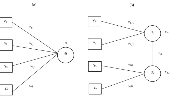
Another derivation of LMA models as item response models was given by Anderson and Yu (2007). Their derivation is based on Anderson and Vermunt (2000)’s LMA model as latent variable models for observed data, which use statistical graphical models for discrete and continuous variables (Lauritzen & Wermuth, 1989). They also showed that the LMA models derived in Anderson and Vermunt (2000) are formally equivalent to models in Holland (1990). For illustration, consider the following two graphs for uni- and multidimensional models presented in Figure 1.

Graph (A) represents a unidimensional model where four items are directly related to only one latent variable, and Graph (B) represents a multidimensional model where each half of four items are directly related to one of two latent variables and those two latent variables are correlated. Each item (i.e., discrete variable) is represented by a square and the latent variables by circles. If two variables are not connected by a line, those variables are independent given all the other variables in the graph. If there is a line connecting two variables, it indicates that they may be (conditionally) dependent. Since no line directly connects any two items in either Graph

16

Figure 1. Graphs for (A) one latent variable and (B) two correlated latent variables with four items

(A) or (B), given the latent variables, items are conditionally independent (i.e., local independence).

Anderson and Yu (2007) showed that the assumptions made by Anderson and Vermunt (2000) were the same as those that Holland (1990) made. In addition to assuming the marginal distribution of response patterns is multinomial, there are two major assumptions for the model, which Anderson and Yu (2007) recounted from the perspective of the graphical model:

(a) The responses to items (observed variables) are conditionally independent given the latent continuous ones :

𝑝(𝒚|𝜃) = P(𝐘 = 𝐲|𝚯 = 𝜃) = ∏ 𝑝(𝒀_𝑖 = 𝑦_𝑖|𝜃). 𝐼

𝑖=1

(b) The joint distribution of observed and latent continuous variables is a

homogenous conditional Gaussian distribution (Lauritzen & Wermuth, 1989). A homogenous

Y1 Y2 Y3 Y4 Θ1 𝜈1𝑗1 𝜈2𝑗1 𝜈3𝑗2 𝜈4𝑗2 Θ2 𝜎12 𝜎22 𝜎11 Y1 Y2 Y3 Y4 Θ 𝜈1𝑗 𝜈2𝑗 𝜈3𝑗 𝜈4𝑗 σ (A) (B)

17

conditional Gaussian distribution is the distribution of the continuous variables (i.e., θ) given the response pattern (i.e., y) is normal. The mean depends on the response pattern given but the variance remains the same over response patterns :

Θ|𝐘 = 𝒚⁡is⁡𝑁(𝜇_𝒚, ⁡𝜎2_)⁡.

Following Anderson and Vermunt (2000) and Anderson and Böckenholt (2000), Anderson and Yu (2007) showed the joint distribution of observed and latent continuous variables, which is restated below.

𝑓(𝒚, 𝜃) = 𝑓(𝜃|𝒚)𝑷(𝒚) = 1 √2𝜋𝜎2exp [− (𝜃 − 𝜇_(𝒚))2 2𝜎2 ] 𝑷(𝒚) = exp [𝑔(𝒚) + ℎ(𝒚)𝜃 − 𝜃2 2𝜎2]⁡, (2.8) where _{𝑔(𝒚) = log (} 1 √2𝜋𝜎2) + log(𝑷(𝒚)) − 𝜇_(𝒚)2 2𝜎2⁡⁡, (2.9) and ℎ(𝒚) = 𝜇𝒚/𝜎2⁡. (2.10)

The distribution in (2.8) is a homogeneous conditional Guassian distribution.

In Anderson and Vermunt (2000), 𝑔(𝒚) represents the dependencies among discrete variables (i.e., item responses to items) given the latent variable and ℎ(𝒚) shows the

dependencies between discrete variables and the latent variable. By rewriting 𝑔(𝒚) in equation (2.9) in terms of log(𝑷(𝒚)), the log manifest probabilities for response pattern are obtained, that is,

log(𝑷(𝒚)) = 𝑔(𝒚) + log (√2𝜋𝜎2_{) +}𝜇(𝒚) 2

18

To derive LMA model for log manifest probabilities for response pattern, Anderson and Vermunt (2000) specified definitions for 𝑔(𝒚) and ℎ(𝒚). By the assumption of conditional independence of item responses given the latent variable, 𝑔(𝒚) is set equal to the sum of location parameters for each item, that is,

𝑔(𝒚) = ∑ 𝜆_𝑖𝑗⁡. 𝐼

𝑖=1

(2.12) As presented in equation (2.8), ℎ(𝒚) is a function of coefficients that shows the strength of the relationship between item responses to each item and the latent variable and is defined as the sum of category scores for each item, that is,

ℎ(𝒚) = ∑ 𝜈𝑖𝑗⁡. 𝐼

𝑖=1

(2.13)

By the two definitions of ℎ(𝒚) in (2.10) and (2.13), the mean of the homogenous conditional Gaussian distribution is defined as a linear expansion of scores, which equals:

𝜇𝒚= 𝜎2∑ 𝜈𝑖𝑗⁡. 𝐼

𝑖=1

(2.14) By substituting (2.12) and (2.14) into equation (2.11), the LMA model for the log

manifest probabilities of response pattern can be rewritten as

log(𝑷(𝒚)) = 𝜆 + ∑ 𝜆𝑖𝑗 + 𝜎2∑ ∑ 𝜈𝑖𝑗 𝑖<𝑘 𝜈𝑘𝑗 𝑖 𝑖 ⁡, _(2.15)

where λ is a normalizing parameter that ensures that the P(y) sum to 1 over response patterns, 𝜆_𝑖𝑗 are the marginal effect term for category j on item i, 𝜈_𝑖𝑗 are category scale values or scores for category j on item i, and 𝜎2 is an association parameter (i.e., variance of conditional distribution of θ) that shows the strength of the relationship between the items.

19

Anderson and Yu (2007) showed the equivalence of the LMA model using statistical graphical models to the one derived by Holland (1990) using the Dutch identity by showing that the above assumptions are equivalent to those made by Holland. When deriving the Dutch identity for the manifest probabilities of response patterns, Holland assumed that item logit functions are linear of a latent variable (θ). Anderson and Yu (2007) showed that the same assumption was also made in the LMA model by showing that item discrimination and item difficulty parameters of item logit functions can be rewritten as the difference between the corresponding parameters (i.e., 𝜈_𝑖𝑗 and 𝜆_𝑖𝑗, respectively) of the LMA models. Another

assumption made by Holland is that the posterior distribution of θ is normal with the mean and the variance for one response pattern (𝒚0). Anderson and Yu (2007) also proved that if it is the

case for 𝒚₀,⁡then it is true for all response patterns (see also Hessen, 2012). In addition to these two assumptions, conditional independence and a multinomial distribution for the manifest probabilities of response patterns are also assumed in both derivations. The equivalence of the assumptions between both approaches has further established that LMA models can function as item response models.

Fully Conditional Specification Derivation of LMA Models

Anderson and Yu (2007) provided a new derivation of LMA model as item response models based on fully conditionally specified logistic regression models using a rest-score in lieu of θ. The sum of responses to items weighted by category scores (i.e.,⁡𝜈_𝑖𝑗) are sufficient statistics for the latent variable (Andersen, 1995; Ostini & Nering, 2006). Adapting the idea with a slight change, Anderson and Yu (2007) (see also Anderson, Li, & Vermunt, 2007; Anderson,

20

latent variable based on the precedence and justification for it in the literature on classical test theory and IRT as mentioned in Junker and Sijtsma (2000).

A rest-score is the sum of all the item scores except for the item being studied. For example, Graph (A) in Figure 1 represents a case where all of the four items are directly related to the only one latent variable, θ (i.e., unidimentional model). When modeling the response to item 1 in Graph (A), the sum of the responses of Y2, Y3, and Y4 would be used as an estimate of θ; that is,

𝜃̃−1= 𝜎11(𝜈2𝑗+ 𝜈3𝑗+ 𝜈4𝑗)⁡. (2.16)

The symbol 𝜃̃₋₁ represents the estimate of θ and is referred to as a rest-score for item 1. The subscript, ‘-1’ indicates that the response of item 1 is not included in the estimate of θ. The sum, (𝜈_2𝑗+ 𝜈_3𝑗+ 𝜈_4𝑗), is over the category scores of all the other items except for the item that is being modeled (i.e., item 1) and 𝜎₁₁ is an association parameter which is the variances of θ within a response pattern.

When defining a rest-score in the case of multiple correlated latent variables, it consists of two components: (a) the one that is directly related to the latent variable and (b) the one that (indirectly) relates to the information from the correlated latent variable(s) with the target latent variable (Anderson, Li, & Vermunt, 2007; Anderson, Verkuilen, & Peyton, 2010; Anderson, 2013). The latter adds to estimation of 𝜃̃_−𝑖. De la Torre and Patz (2005) found that taking into account the correlation between abilities can lead to a great improvement in ability estimation. Wang, Chen, and Cheng (2004) reported that using item responses to other tests as collateral information ca n increase measurement efficiency when the target ability is estimated.

Graph (B) in Figure 1 shows a simple multidimensional structure with four items and two correlated variables. Items 1 and 2 are directly related to 𝜃₁, and items 3 and 4 to ⁡𝜃₂, and two

21

latent variables are correlated. When specifying a model for Y1, only the response of Y2 would be taken as an estimate of 𝜃₁. Since two latent variables, 𝜃₁ and 𝜃₂ are correlated and items 3 and 4 are direct indicators of 𝜃2, it would be possible to get some information about 𝜃1 from them.

Thus, the responses of Y3 and Y4 would also be included in modeling 𝜃₁. Therefore, the rest-score for item 1, namely, the estimate of 𝜃₁ in modeling the response of Y1 under two correlated latent variables,

𝜃̃_1,−1 = 𝜎₁₁(𝜈_2𝑗1) + 𝜎₁₂(𝜈_3𝑗2+ 𝜈_4𝑗2)⁡. (2.17) The more general form for any number of latent variables is

𝜃̃_𝑚,−𝑖 = 𝜎_𝑚𝑚∑ 𝜈_𝑘𝑗𝑚 𝑘≠𝑖 + ∑ 𝜎_𝑚𝑚′ 𝑚′_≠𝑚 (∑ 𝜈_𝑘𝑗𝑚′ 𝑘 )⁡, (2.18)

where 𝜃̃_𝑚,−𝑖 indicates the estimate of θ for the latent variable m that excludes the response of item i, 𝜈𝑘𝑗𝑚 is the category score for the response j on item k, which isa direct indicator ofthe

latent variable m, 𝜎_𝑚𝑚 is a weight (variance) that reflects the scale of the latent variable m, and

𝜎_𝑚𝑚′ is a weight that shows the strength of the relationship between latent variables (i.e., covariance).

Replacing θ with its estimator 𝜃̃𝑚,−𝑖 in equation (2.18) yields a set of fully conditional

multinomial logistic regression models, one for each item. For illustration, the example model in Graph (B) in Figure 1 is used;

Item 1 : P(𝑌1= 𝑗|𝜃̃1,−1) = exp⁡{𝜆1𝑗+ 𝜈1𝑗1(𝜎11𝜈2𝑗1+ 𝜎12(𝜈3𝑗2+ 𝜈4𝑗2))}/𝑘1 (2.19)

Item 2 : P(𝑌₂ = 𝑗|𝜃̃_1,−2) = exp⁡{𝜆_2𝑗+ 𝜈_2𝑗1(𝜎₁₁𝜈_1𝑗1+ 𝜎₁₂(𝜈_3𝑗2+ 𝜈_4𝑗2))}/𝑘₂ (2.20) Item 3 : P(𝑌₃ = 𝑗|𝜃̃_2,−3) = exp⁡{𝜆_3𝑗 + 𝜈_3𝑗2(𝜎₂₂𝜈_4𝑗2+ 𝜎₁₂(𝜈_1𝑗1+ 𝜈_2𝑗1))}/𝑘₃ (2.21) Item 4 : P(𝑌₄ = 𝑗|𝜃̃_2,−4) = exp⁡{𝜆_4𝑗 + 𝜈_4𝑗2(𝜎₂₂𝜈_3𝑗2+ 𝜎₁₂(𝜈_1𝑗1+ 𝜈_2𝑗1))}/𝑘₄⁡ , (2.22) where 𝑘𝑖 = ∑ exp⁡(𝜆𝑗ℎ 𝑖ℎ + 𝜈𝑖ℎ𝑚𝜃̃𝑚,−𝑖).

22

For any number of items and multiple latent variables, the set of fully conditionally specified response functions is defined as

P(𝑌𝑖 = 𝑗|𝜃̃𝑚,−𝑖)

= exp {𝜆𝑖𝑗 + 𝜈𝑖𝑗𝑚(𝜎𝑚𝑚∑𝑘≠𝑖𝜈𝑘𝑗𝑚+ ∑𝑚≠𝑚′𝜎𝑚𝑚′(∑ 𝜈𝑘 𝑘𝑗𝑚′))} ∑ exp {𝜆𝑗_ℎ 𝑖ℎ + 𝜈𝑖ℎ𝑚(𝜎𝑚𝑚∑𝑘≠𝑖𝜈𝑘𝑗𝑚+ ∑_𝑚≠𝑚′𝜎𝑚𝑚′(∑ 𝜈_{𝑘 𝑘𝑗𝑚}′))}

⁡ for i =1, 2, .., I. (2.23)

The models above are called ‘fully conditionally specified models’ because the response of each item is modeled conditional on all of the other items. To estimate the parameters of the observed response patterns of items by fitting the set of conditional logistic regression models, the joint distribution for the manifest probabilities of the response patterns, P(y) will be found (except for

𝜆_𝑖𝑗).

A set of fully conditional specification of models (Anderson & Yu, 2007; Anderson, Li, & Vermunt, 2007; Anderson, Verkuilen, & Peyton, 2010) over-determines the joint distribution (Anderson, 2013; Gelman & Speed, 1993). Joe and Liu (1996) used the conditional specification method for multivariate binary response data with covariates and provided necessary and

sufficient conditions for compatibility of conditional distributions. According to them, when one binary response variable, 𝑌_𝑖 is conditional on 𝑌_𝑗⁡(𝑖 ≠ 𝑗) and vice versa the two-way interaction parameters between two variables, 𝛾_𝑖𝑗 and 𝛾_𝑗𝑖 must be equal for the conditional distributions to be compatible or consistent. Extending Joe and Liu’s results to polytomous multidimensional IRT models, Anderson, Li, and Vermunt (2007), Anderson, Verkuilen, and Peyton (2010), and Anderson (2013) showed that this condition also holds for a set of fully conditionally specified models, including those that contained covariates and imposed ordinal constraints or parameters. The set of conditional models uniquely leads to an LMA model for the observed response

23

The LMA model for response patterns corresponding to Model (2.19) through (2.22), which corresponds to Graph (B) in Figure 1 is

log 𝑃(𝑦) = 𝜆 + 𝜆_1𝑗 + 𝜆_2𝑗 + 𝜆_3𝑗+ 𝜆_4𝑗 + 𝜎11𝜈1𝑗1𝜈2𝑗1+ 𝜎22𝜈3𝑗2𝜈4𝑗2

+ 𝜎12(𝜈1𝑗1𝜈3𝑗2+ 𝜈1𝑗1𝜈4𝑗2+ 𝜈2𝑗1𝜈3𝑗2+ 𝜈2𝑗1𝜈4𝑗2)⁡.

(2.24)

The more general form of LMA model for the joint distribution is;

log 𝑃(𝒚) = 𝜆 + ∑ 𝜆𝑖𝑗 + ∑ ∑ ∑ ∑ 𝜎𝑚𝑚′𝜈_𝑖𝑗𝑚 𝑚≥𝑚′ 𝜈_𝑘𝑗𝑚′⁡⁡, 𝑚 𝑖>𝑘 𝑖 𝑖 (2.25) where y is the response pattern on I items, 𝜆 ensures that the sum of the probabilities over all the possible response patterns equals 1, 𝜆𝑖𝑗 represents the marginal effect terms of each category on

item i, and 𝜎_𝑚𝑚′𝜈_𝑖𝑗𝑚𝜈_𝑘𝑗𝑚′ is the multiplicative term of category scores between pairs of items with an association parameter. In the case where item k is not directly related the latent variable

m, the corresponding 𝜈_𝑘𝑗𝑚 will be set to zero. For example, since there is no relationship between item 2 and 𝜃2 in Graph (B), its category scores for the latent variable 𝜃2, 𝜈2𝑗2 equals

zero.

As mentioned earlier, LMA models are special cases of log-linear models (a Possion regression) with only two-way interaction terms. Multinomial logistic regression models with categorical variables for predictors can be written in the form of log-linear models (Agresti, 2002). Therefore, each parameter in LMA model given in equation (2.24) is the same as those in equations (2.19) through (2.22) for multinomial logistic models. That is, the marginal effect terms, 𝜆_𝑖𝑗 correspond to the location parameters in the multinomial logistic regression models,

24

and the product terms of weights (𝜎_𝑚𝑚′) and category scores (𝜈_𝑖𝑗𝑚)⁡also appear in both equations.

There are two great advantages in the LMA model as item response model derived by Anderson, Verkuilen, and Peyton (2007). First, since LMA models are equivalent to Possion regression models, not only can the parameters be estimated without using numerical integration, but also explicit assumptions regarding the marginal distribution of the latent variables are not necessary. The LMA models allow IRT models with multiple latent variables to be fit to data using MLE by using computer software such as lEM (Vermunt, 1997) and PROC/NLP in SAS.

A second of advantage of the fully conditional specification approach is that it suggests how parameters for large numbers of items could be estimated in an efficient way that

overcomes the limitations of MLE of LMA models. The parameters of LMA models are estimated by MLE and it requires iteratively computing fitted values for all possible response patterns. ML estimates of LMA models for small numbers of items can be obtained easily, but the standard estimation methods for large numbers of items fail because the number of possible response patterns increases exponentially as the number of items and response options per item increase. Rather than MLE, pseudo-likelihood estimation can be done and will be discussed in the following chapter.

25 Chapter 3

Estimation of LMA Models

Log-linear and LMA models are typically estimated by maximum likelihood estimation (MLE). This chapter provides an overview of the estimation procedures of the parameters in LMA models. Two estimation procedures for LMA models as MIRT models will be introduced, maximum likelihood estimation and pseudo-likelihood estimation, followed by its

implementation for LMA Rasch models (i.e., linear-by-linear models). The more general algorithm will be presented in the Chapter 4.

Maximum Likelihood Estimation (MLE)

Let C denote the number of possible item response patterns y, 𝑃(𝒚𝑐) denote their

probabilities, where ∑ 𝑃(𝒚_{𝑐 𝑐})= 1, and 𝑛(𝒚_𝑐) denote the number of examinees in the sample having a response pattern 𝒚_𝑐, where ∑ 𝑛(𝒚_{𝑐 𝑐})= 𝑁, total number of examinees in the sample. Then, {𝑛(𝒚_𝑐)}⁡follows a multinomial distribution with parameters N and 𝑃(𝒚_𝑐) as below:

𝑃[𝑛(𝒚₁), 𝑛(𝒚₂), 𝑛(𝒚₃), … , 𝑛(𝒚_𝑐)] = ( 𝑁! 𝑛(𝒚₁)! 𝑛(𝒚2)! 𝑛(𝒚3)! … 𝑛(𝒚𝑐)!) 𝑃(𝒚1) 𝑛(𝒚1)_𝑃(𝒚 2)𝑛(𝒚2)𝑃(𝒚3)𝑛(𝒚3)… 𝑃(𝒚𝑐)𝑛(𝒚𝑐)⁡⁡. (3.1)

Removing a multiplicative constant, the kernel of the likelihood function for multinomial count data of item response patterns equals

𝐿 = ∏exp⁡(−𝑃(𝒚𝑐))𝑃(𝒚𝑐) 𝑛(𝒚𝑐) 𝑛(𝒚𝑐)! 𝐶 𝑐=1 ⁡, (3.2)

and the kernel of the log-likelihood function is

log 𝐿 = ∑ 𝑛(𝒚𝑐) log 𝑃(𝒚𝑐) − 𝑃(𝒚𝑐) 𝐶

𝑐=1

26

Holland (1990) showed that fitting IRT models by MMLE based on an item response matrix which presents all the responses to I items of all examinees in the sample (i.e., N) is equivalent to fitting a second-order log-linear model for multinomial count data by MLE (Holland, 1990) and this goes the same for LMA models.

Computer Programs for Parameter Estimation in LMA Models

There are a number of computer programs for fitting LMA models and these include

l

them,

l

l

conducts parameter estimation of LMA models by maximum likelihood using a quasi-Newton algorithm. Uni-dimensional Newton-Raphson algorithm is a variant of Newton-Raphson

algorithm that only uses the diagonal elements of the Hessian matrix to update equations for the parameters. Global optimal solutions are not guaranteed but multiple runs with random starts can be used to check convergence. For details, see Anderson and Vermunt (2000). PROC/NLP in SAS provides a variety of ways for estimating parameters in nonlinear statistical models. Both unconstrained and constrained maximization/minimization problems can be handled by the procedure with a set of optimization methods, including Newton-Raphson and quasi-Newton method. The latter is used when non-linear constraints are placed on parameters, otherwise Newton-Raphson can be used, which does give a unique global maximum. LMA models can be fit to data easily with three command statements in PROC/NLP. They are: (a) ‘parms’ statement that specifies the parameters to be estimated, (b) the equation of an LMA model, and (c) the logarithm of the likelihood function to be maximized. With Newton-Raphson, it yields estimates

27

of standard errors and covariance matrices for parameter estimates. These features of PROC/NLP provide an easy and flexible way of fitting LMA models.

Motivation of PLE for LMA models

When estimating parameters in LMA models with MLE, it requires iteratively computing fitted values for all possible response patterns. Parameter estimates of LMA models for small numbers of items can be obtained by MLE easily because the number of all possible response patterns is reasonable. For large numbers of items, however, the standard estimation methods of LMA models fail because the number of possible response patterns increases exponentially as the number of items and response options per item increase. For example, Anderson (2013) reported that the estimation of an LMA model for 8 items with 5 categories using PROC/NLP was successful, but failed for 9 items with the same number of categories. The number of possible item response patterns for 8 items equals 58 = 390,625⁡and it increases to 59 =

1,953,125⁡ when just one item is added to 8 items, which makes the MLE of LMA models infeasible.

More recently, pseudo-likelihood estimation (PLE) was proposed to solve the problem for Rasch models with large numbers of items (Anderson, Li, & Vermunt 2007; Li 2010). It is reported that PLE can fit the models to data with large numbers of items successfully and fast, handle models with multiple latent variables and covariates, yield consistent estimates, and is easy to implement.

Pseudo-likelihood Estimation (PLE)

Pseudo-likelihood estimation (PLE) was first introduced by Besag (1974) as an approach to the specification and estimation of spatial interaction models. He pointed out that a

28

maximum likelihood. To solve this problem, he specified a conditional distribution for spatial data observed at a specific site given the data observed at all the other sites and obtained the parameter estimates by maximizing the product of the conditional likelihood functions for data. As shown in his study, the basic idea behind PLE is to replace numerically challenging problems with more tractable ones by simplifying them with conditional specification approach so that computational demands can decrease in fitting models. For its computational efficiency, PLE has been used as an alternative to maximum likelihood estimation in a number of studies on social networks (Strauss & Ikeda, 1990; Wasserman & Pattison, 1990), multivariate clustered data (Geys, Molenberghs, & Ryan, 1999; Molenberghs & Verbeke, 2005), longitudinal data (Troxel, Lipsitz, & Harrington, 1998; Parzen, Lipsitz, Fitzmaurice, Ibrahim, Troxel, & Molenberghs, 2007), incomplete data (Molenberghs, Kenward, Verbeke, & Birhanu, 2011).

Several studies have been performed to estimate parameters of Rasch models with PLE (Arnold & Strauss, 1991; Strauss, 1992; Zwinderman, 1995; Smit & Kelderman, 2000).

Following Besag (1974, 1975)’s conditional approach, Arnold and Strauss (1991) and Strauss (1992) provided the definition of pseudo-likelihood for pairs of binary items using Rasch models and mentioned that maximizing the pseudo-likelihood function is equivalent to finding MLE with a logistic regression procedure.

Zwinderman (1995) conducted a simulation study to investigate the consistency and efficiency of PL estimates for Rasch models using responses to pairs of items, irrespective of other items. He compared the estimates from PLE to those from conditional maximum likelihood (CML) and marginal maximum likelihood (MML) estimation methods and showed that PL estimates are consistent and similar in efficiency to CML and MML estimates.

29

Smit and Kelderman (2000) proposed to apply PLE method to Rasch models for binary items. Unlike the pairwise estimation method used by Arnold and Strauss (1991), Strauss (1992), and Zwinderman (1995), they estimated the parameters for Rasch models based on a set of binary item responses and showed that PLE method is more computationally attractive than CML and its estimates are almost identical to CML and unconditional ML estimates.

To summarize, the studies have shown that PLE can be used for Rasch models as an alternative estimation method to MLE, but their application of PLE was limited to

unidimensional binary Rasch models.

PLE for LMA Rasch Models Using Fully Conditionally Specified Models

More recently, Anderson, Li, and Vermunt (2007) proposed PLE for LMA models to solve the problem of MLE for large numbers of items. Like the previous application of PLE to Rasch model, their methodology was also applied to LMA Rasch models, but its application was extended to the models for polytomous items and multiple latent variables. Their implementation of PLE of LMA Rasch models reflects the original idea of PLE introduced by Besag (1974, 1975). As mentioned earlier, fitting LMA models for large numbers of items with MLE is prohibitive due to the exponential increase in the number of all possible item response patterns. To solve this complex problem, they replaced LMA Rasch models for large numbers of items with simpler conditional multinomial logistic models based on fully conditional specification approach (Anderson & Yu, 2007; Anderson, Li, & Vermunt, 2007; Anderson, Verkuilen, & Peyton, 2010). They specified conditional models corresponding to each item using rest score in lieu of the latent variable and defined pseudo-likelihood as the product of the likelihoods of the conditional multinomial logistic regressions. For implementation of PLE, the whole set of fully conditionally specified logistic regression models were “stacked” into a large design matrix and

30

the model parameters were estimated by finding the maximum value of likelihood function with one large stacked conditional multinomial logistic regression model. The maximum value of the likelihood of the model fit to the stacked data equals the maximum of pseudo-likelihood

function.

For illustration, let’s take an example model for a LMA Rasch model with I polytomous items and one latent variable. The graph for the model looks similar to Graph (A) in Figure 1 represented in the previous chapter.

Figure 2. LMA Rasch model with I polytomous items and one latent variable

In Anderson, Verkuilen, and Peyton (2010)’s fully conditional specification approach, the rest score for item i is defined as

𝜃̃_−𝑖 = 𝜎₁₁∑ 𝜈_𝑘𝑗 𝑘≠𝑖

⁡. _(3.4)

where 𝜃̃−𝑖 indicates the estimate of θ (e.g., a rest score) for item i, 𝜈𝑘𝑗 is the known (or

assumed) category score for the response j on item k, and 𝜎₁₁ is a weight (variance) that reflects the scale of the latent variable within response patterns.

Y1 Y2 YI-1 YI Θ 𝜈1𝑗 𝜈2𝑗 𝜈(𝐼−1)𝑗 𝜈𝐼𝑗 𝜎11 .... .

31

Using the defined weighted rest score in equation (3.4), the LMA Rasch model in Figure 2 yields a set of fully conditionally specified multinomial logistic regression models:

P(𝑌₁ = 𝑗|𝜃̃₋₁) = exp⁡{𝜆_1𝑗+ 𝜈_1𝑗(𝜎₁₁∑ 𝜈_𝑘𝑗 𝑘≠1 )}/𝑘₁ (3.5) P(𝑌₂ = 𝑗|𝜃̃₋₂) = exp⁡{𝜆_2𝑗+ 𝜈_2𝑗(𝜎₁₁∑ 𝜈_𝑘𝑗 𝑘≠2 )}/𝑘₂ (3.6) : = : P(𝑌_𝐼 = 𝑗|𝜃̃_−𝐼) = exp⁡{𝜆_𝐼𝑗+ 𝜈_𝐼𝑗(𝜎₁₁∑ 𝜈_𝑘𝑗 𝑘≠𝐼 )}/𝑘_𝐼⁡⁡, (3.7) where 𝑘_𝑖 = ∑𝑗_ℎ=0exp⁡{𝜆_𝑖ℎ+ 𝜈_𝑖ℎ(𝜎₁₁∑_𝑘≠𝐼𝜈_𝑘𝑗)}.

As defined earlier, pseudo-likelihood is the product of the likelihoods of the conditional multinomial logistic regressions. Therefore, pseudo-likelihood for person n is defined as

𝑃𝐿⁡(𝝀|𝒚𝑛) = ∏ P(𝑌𝑛𝑖 = 𝑗|𝜃̃𝑛(−𝑖)) 𝐼 𝑖=1 = ∏ exp⁡{𝜆𝑖𝑗+ 𝜈𝑖𝑗(𝜎11∑𝑘≠𝑖𝜈𝑘𝑗)} ∑𝑗_ℎ=0exp⁡{𝜆_𝑖ℎ+ 𝜈_𝑖ℎ(𝜎₁₁∑_𝑘≠𝑖𝜈_𝑘𝑗)} 𝐼 𝑖=1 ⁡⁡⁡, (3.8)

where 𝝀 is the vector of parameters in the model and 𝒚_𝑛 is a response pattern to I items of person

n.

Assuming that each person is independent, pseudo-likelihood for all persons in N is expressed as

𝑃𝐿⁡(𝝀|𝒚₁, 𝒚₂, … 𝒚_𝑁) = ∏ ∏ P(𝑌𝑛𝑖 = 𝑗|𝜃̃𝑛(−𝑖)) 𝐼 𝑖=1 𝑁 𝑛=1 = ∏ ∏ exp⁡{𝜆𝑖𝑗 + 𝜈𝑖𝑗(𝜎11∑𝑘≠𝑖𝜈𝑘𝑗)} ∑𝑗_ℎ=0exp⁡{𝜆𝑖ℎ+ 𝜈𝑖ℎ(𝜎11∑𝑘≠𝑖𝜈𝑘𝑗)} 𝐼 𝑖=1 𝑁 𝑛=1 ⁡⁡⁡. (3.9)

By taking logarithms on both sides of equation (3.9), log pseudo-likelihood for the whole response patterns of all individuals can be expressed as