COMPUTATIONALLY EFFICIENT
GOODNESS-OF-FIT TESTS
FOR THE ERROR DISTRIBUTION
IN NONPARAMETRIC REGRESSION
Authors: G.I. Rivas-Mart´ınez
– Laboratorio de Sistemas de Potencia y Control, Universidad Nacional de Asunci´on, Paraguay [email protected]
M.D. Jim´enez-Gamero
– Dpto. de Estad´ıstica e Investigaci´on Operativa, Universidad de Sevilla, Espa˜na
Received: April 2016 Revised: August 2016 Accepted: August 2016
Abstract:
• Several procedures have been proposed for testing goodness-of-fit to the error distri-bution in nonparametric regression models. The null distridistri-bution of the associated test statistics is usually approximated by means of a parametric bootstrap which, under certain conditions, provides a consistent estimator. This paper considers a goodness-of-fit test whose test statistic is anL2 norm of the difference between the empirical characteristic function of the residuals and a parametric estimate of the characteristic function in the null hypothesis. It is proposed to approximate the null distribution through a weighted bootstrap which also produces a consistent estimator of the null distribution but, from a computational point of view, is more efficient than the parametric bootstrap.
Key-Words:
• goodness-of-fit; empirical characteristic function; regression residuals; weighted boot-strap; consistency.
AMS Subject Classification:
1. INTRODUCTION
Let (X, Y) be a bivariate random vector satisfying the general nonpara-metric regression model
(1.1) Y =m(X) +σ(X)ε,
where m(x) =E(Y|X=x) is the regression function, σ2(x) = Var(Y |X=x)
is the conditional variance function andεis the regression error, which is assumed to be independent of X. Note that, by construction, E(ε) = 0 and Var(ε) = 1. The covariate X is continuous with density function fX. The regression
func-tion, the variance funcfunc-tion, the error distribution and that of the covariate are unknown and no parametric models are assumed for them.
Because the knowledge of the error distribution will improve the statistical analysis of model (1.1), several authors have proposed tests for such distribution, that is, tests of the null hypothesis
H0:F ∈ F,
versus the alternative
H1:F /∈ F,
where F stands for the cumulative distribution function (CDF) of εand F is a parametric family,
F =
F(·;θ), θ∈Θ , Θ⊆Rp.
Examples are the tests in Neumeyeret al.[17] and Heuchenne and Van Keilegom [6], which are based on comparing the empirical CDF of the residuals to a para-metric estimator of the CDF under the null hypothesis. Since the equality of the CFDs can be also interpreted in terms of the associated characteristic functions (CFs), Huˇskov´a and Meintanis [11] have proposed a test for H0 that is based on
comparing the empirical CF of the residuals to a parametric estimator of the CF under the null hypothesis. As commented in Jim´enez-Gamero [13], it is interes-ting to observe that the last paper requires weaker conditions for the validity of the procedures than the ones based on the CDF. Nevertheless, in all cases the limit distribution of the proposed test statistics is unknown, even under the null distribution, because it depends on the unknown value of the parameter θ. To overcome this difficulty, these papers propose to use a parametric bootstrap (PB) for approximating the null distribution of the test statistic. Although very easy to implement, the PB can become very computationally expensive as the sample size and/or the number of unknown parameters increase.
This paper studies another method for estimating the null distribution of the test statisticTn,w(ˆθ) in [11]. Specifically, a weighted bootstrap (WB)
has been previously suggested in Kojadinovic and Yan [15], to approximate the null distribution of goodness-of-fit (GOF) tests based on the empirical CDF, and in Jim´enez-Gamero and Kim [14], to approximate the null distribution of GOF tests based on the empirical CF (ECF), among others. Both papers assume ob-servable independent and identically distributed (IID) data. They show that the properties of the WB are quite similar to those of the PB (it provides a con-sistent estimator of the null distribution and the resulting test is able to detect any alternative) but, from a computational point of view, it is more efficient. In view of the good properties of the WB in these and other papers, it is also expected to work satisfactorily for estimating the null distribution of the test statistic considered in this paper. The purpose of the current study is to investi-gate, both theoretically and empirically, the use of the WB for approximating the null distribution of Tn,w(ˆθ). A main difference between the setting in this paper
and the one in [14, 15] is that in our case the errors are not observable. So we replace the errors by the residuals, but the residuals are not independent.
The paper is organized as follows. Section 2 describes the test statistic and explains some problems with the WB approximation. Section 3 gives a solution to the problems described in the previous section and proves the consistency of the proposed WB approximation. It also shows that the resulting test is consistent, in the sense of being able to detect any alternative. The application of the proposed WB approximation requires the estimation of certain functions appearing in the linear expansion of the parameter estimators. The estimation of such functions is dealt with in Section 4. Section 5 reports the results of some simulation experiments designed to study the finite sample performance of the proposed approximation and to compare it to the PB. From this numerical study it is concluded that both approximations behave quite closely but, from a computational point of view, the WB outperforms the PB. Section 6 concludes and outlines possible extensions of the results presented in this paper. All proofs and technical details are deferred to the last section.
The following notation will be used along the paper: all vectors are col-umn vectors; for any vector a, ak denotes its k-th coordinate and kak its
Eu-clidean norm; the superscript T denotes transpose; E
θ and Pθ denote
expec-tation and probability, respectively, assuming that the data has CDF F(·;θ);
P∗ denotes the conditional probability law, given the data; all limits in this paper are taken when n→ ∞; →L denotes convergence in distribution; →P de-notes convergence in probability; a.s.→ denotes the almost sure convergence; for any complex number z=a+ ib, |z| is its modulus; an unspecified integral de-notes integration over the whole real line R; for a given non-negative real-valued
function w we denote k · kw to the norm andh·,·iw to the scalar product in the
Hilbert space L2(w) ={g:R→C,R |g(t)|2w(t)dt <∞}; if F is a CDF, then L2(F) ={g:R→C,R
|g(t)|2dF(t)<∞}; for any real function f(t;θ) differen-tiable at t∈R and at θ= (θ1, θ2, ..., θp)T ∈Rp the following notations will be
used: f′(t;θ) = ∂ ∂tf(t;θ), f(r)(t;θ) = ∂ ∂θr f(t;θ), 1≤r ≤p, ∇f(t;θ) =f(1)(t;θ), f(2)(t;θ), ..., f(p)(t;θ) T .
2. THE TEST STATISTIC
Let (X1, Y1), ...,(Xn, Yn) be IID from model (1.1), that is, Yj =m(Xj) +
σ(Xj)εj, 1≤j≤n. Since the hypothesisH0is on the common error distribution,
ε1, ..., εn, and the errors are not observable, the inference must be based on the
residuals, ˆ εj = Yj−mˆ(Xj) ˆ σ(Xj) , 1≤j≤n,
where ˆm(·) and ˆσ(·) are estimators ofm(·) andσ(·), respectively. Several choices are possible for ˆm(·) and ˆσ(·). Here, as in [11], we use the following kernel estimators for the density functionfX ofX, the regression functionm(·) and the
variance functionσ2(·), ˆ fX(x) = 1 n n X j=1 Khn(Xj −x), ˆ m(x) = 1 nfˆX(x) n X j=1 Khn(Xj−x)Yj, ˆ σ2(x) = 1 nfˆX(x) n X j=1 Khn(Xj−x){Yj −mˆ(x)} 2, where Khn(·) = 1 hnK( ·
hn), K(·) is a kernel and hn is the bandwidth, satisfying
certain conditions that will be specified later.
Huˇskov´a and Meintanis [11] proposed the following test for testingH0,
Ψ =
(
1, if Tn,w(ˆθ)≥tn,ω,α,
0, otherwise,
where tn,ω,α is the 1−α percentile of the null distribution ofTn,ω(ˆθ),
(2.1) Tn,ω(ˆθ) =n
Z
|cn(t)−c(t,θˆ)|2ω(t)dt=nkcn(t)−c(t,θˆ)k2w,
cn(t) is the ECF of the residuals,
cn(t) = 1 n n X j=1 exp(itεˆj) = 1 n n X j=1 cos(tεˆj) + i 1 n n X j=1 sin(tεˆj),
c(t;θ) is the CF associated to F(ε;θ), that is, c(t;θ) =Eθ{exp(itε)}=R(t;θ) +
iI(t;θ),ω(t) is a nonnegative function such thatR
ω(t)dt <∞, which may depend on θ, and ˆθ is a consistent estimator ofθ satisfying the following assumption.
(A.1) Under H0, √n(ˆθ−θ0) = 1 √n n X j=1 ψ(εj;θ0) +op(1), where θ0 is the
true parameter value,Eθ0{ψ(εj;θ0)}= 0 andEθ0
kψ(εj;θ0)k2 <∞.
Assumption (A.1) implies that, when the null hypothesis is true and θ0
denotes the true parameter value, √n(ˆθ−θ0) is asymptotically normally
dis-tributed. This assumption is satisfied by commonly used estimators such as ma-ximum likelihood estimators and method of moment estimators when ε1, ..., εn
are observable and, in such a case, the expression of the functionψis well-known (see, for example, [1, Ch. 5]). In our setting, the errors are not observable and the expression of the function ψ differs from the observable case. This topic will be discussed in detail in Section 4.
Theorem 1 in [11] states that if ˆθsatisfies (A.1),H0 is true andθ0is the true parameter value, under certain additional conditions (assumptions (A.2)–(A.7) in Section 7),
(2.2) Tn,ω(ˆθ)−→ kL Z(t;θ0)k2ω,
where {Z(t;θ0), t∈R}is a centered Gaussian process on L2(ω) with covariance
structure of the form Covθ0{Z1(ε;t, θ0, ψ), Z1(ε;s, θ0, ψ)},
(2.3) Z1(ε;t, θ, ψ) = cos(tε) + sin(tε)−R(t;θ)−I(t;θ)−tε{R(t;θ)−I(t;θ)}
−tε22−1{R′(t;θ) +I′(t;θ)} −ψT(ε;θ){∇R(t;θ) +∇I(t;θ)}.
Clearly, the asymptotic null distribution of Tn,ω(ˆθ) is unknown. It depends on
the hypothetical the error distribution, on the chosen estimator and the true unknown value of the parameter.
In order to try to approximate the null distribution of Tn,ω(ˆθ) we first
observe that it resembles a degree-2 V-statistic, because
Tn,ω(ˆθ) = 1 n n X j=1 n X k=1 ρ(ˆεj,εˆk; ˆθ), withρ(ε, z;θ) =u(ε−z)−u0(ε;θ)−u0(z;θ) +u00(θ),u0(ε;θ) =R u(ε−z)dF(z;θ), u00(θ) = R u(ε−z)dF(ε;θ)dF(z;θ), andu(t) =R cos(tε)ω(ε)dε.
Dehling and Mikosch [4] (see also Huˇskov´a and Janssen [10]) showed that if
ε1, ..., εn are IID, ξ1, ..., ξn are IID with E(ξ1) = 0 and Var(ξ1) = 1, independent
of ε1, ..., εn and Vn= n12 P
then the conditional distribution, given ε1, ..., εn, of 1 n X 1≤j,k≤n g(εj, εk)ξjξk
consistently estimates that of nVn. In the light of this result, since ˆεj and ˆθ
are approximations to εj and θ, respectively, one may be tempted to estimate
the null distribution of Tn,ω(ˆθ) by means of the conditional distribution, given
(X1, Y1), ...,(Xn, Yn), of (2.4) W∗ = 1 n X 1≤j,k≤n ρ(ˆεj,εˆk; ˆθ)ξjξk.
We will see that this approach is wrong. The next result gives the limit distribu-tion of W∗. The required assumptions are listed in Section 7.
Theorem 2.1. Suppose thatkθˆ−θ1k=op(1), for someθ1 ∈Θ, that
as-sumptions (A.2)–(A.6) hold, that the first partial derivatives R(r)(t;θ),I(r)(t;θ),
1≤r ≤p, exist and are continuous functions∀θ∈U(θ1)⊆Θ, an open
neighbor-hood of θ1, and they are bounded by functions inL2(ω),∀θ∈U(θ1), then
sup
x |P∗{W
∗ ≤x} −P{W0≤x}| P
−→0,
where W0=kZ0(t;θ1)kω2, {Z0(t;θ1), t∈R} is a centered Gaussian process on L2(ω) with covariance structure of the form Cov{Z0(ε;t, θ1), Z0(ε;s, θ1)}, Z0(ε;t, θ) = cos(tε) + sin(tε)−R(t;θ)−I(t;θ).
From the result in Theorem 2.1 and (2.2), it is clear that the conditional distribution ofW∗does not provide a consistent estimator of the null distribution of Tn,ω(ˆθ) because replacing m(·), σ(·) and θ by ˆm(·), ˆσ(·) and ˆθ, respectively,
has an impact on the asymptotic null distribution of the test statistic that is not captured by the conditional distribution of W∗. The next Section shows how to deal with this problem.
Before ending this section we do some comments on the behaviour of ˆθ
under the alternative. Theorem 2.1 assumes that ˆθ has a limit (in probability),
θ1. In practice, to estimate θ one proceeds as ifH0 were true. For example, θis
usually estimated by its quasi maximum likelihood estimator, which maximizes the likelihood under the null hypothesis (with the errors replaced by the resi-duals). IfH0is true, under certain assumptions, the resulting estimator converges
to the true parameter value (see Section 4); if H0 is not true, then proceeding as
in White [22] for observable data, it can shown that, under certain conditions, the estimator also converges to a well-defined limit. Similar comments could be done for other estimators.
3. CONSISTENCY OF THE WB APPROXIMATION
If assumptions (A.1)–(A.7) hold andH0is true, from the proof of Theorem 1
in [11], it follows that (3.1) Tn,ω(ˆθ) =T1,n,ω(θ0) +op(1), where T1,n,ω(θ) =k√1 n n X j=1 Z1(εj;t, θ, ψ)k2ω,
withZ1(ε;t, θ, ψ) as defined in (2.3). Now, from (3.1) and applying the results in [4], we get that the conditional distribution, given (X1, Y1), ...,(Xn, Yn), of
T1∗,n,ω(θ0) =k 1 √ n n X j=1 Z1(εj;t, θ0, ψ)ξjk2ω,
provides a consistent estimator of the distribution of Tn,ω(ˆθ), when H0 is true.
From a practical point of view, this result is useless because Z1(εj;t, θ0, ψ)
de-pends on the non-observable error εj, on the unknown value of θ0 and on the
function ψ(εj;θ0), whose explicit expression is usually unknown. Suppose that kθˆ−θ1k=op(1), for some θ1∈Θ, θ1 being the true parameter value if H0 is
true. To overcome these difficulties we replaceεj by ˆεj,θ0 by ˆθ andψ(εj;θ0) by
ψn(ˆεj; ˆθ), where ψn(·; ˆθ) is a function of the data which approximates ψ in such
a way that (3.2) 1 n n X j=1 kψn(ˆεj; ˆθ)−ψ1(εj;θ1)k2 −→P 0,
with E{kψ1(ε;θ1)k2}<∞ and ψ1(ε;θ1) =ψ(ε;θ1) ifH0 is true.
The choice of ψn will depend on ψ, that is, on the estimator of θ considered.
Section 4 studies some proposals for ψn satisfying (3.2) for two common choices
for ˆθ: the maximum likelihood estimator and the method of moments estimator, both based on the residuals. So, the null distribution ofTn,ω(ˆθ) is now estimated
by means of the conditional distribution, given (X1, Y1), ...,(Xn, Yn), of
T2∗,n,ω(ˆθ) =k√1 n n X j=1 Z1(ˆεj;t,θ, ψˆ n)ξjk2ω.
The next theorem gives the limit of the conditional distribution ofT2∗,n,ω(ˆθ), given (X1, Y1), ...(Xn, Yn).
Theorem 3.1. Suppose thatkθˆ−θ1k=op(1), for someθ1 ∈Θ,θ1 being
the true parameter value if H0 is true, and that assumptions (A.1)–(A.7) and
(3.2)hold, then sup x P∗ n T2∗,n,ω(ˆθ)≤xo−P{T2 ≤x} P −→0,
where T2 =kZ2(t;θ1)k2ω, {Z2(t;θ1), t∈R} is a centered Gaussian process on L2(ω)with covariance structure of the formCov{Z1(ε;t, θ1, ψ1), Z1(ε;s, θ1, ψ1)}.
The result in Theorem 3.1 is valid whether the null hypothesis H0 is true or not. An immediate consequence of this fact and (2.2) is the following.
Corollary 3.1. If H0 is true and the assumptions in Theorem 3.1 hold,
then sup x P∗ n T2∗,n,ω(ˆθ)≤xo−Pθ1 n Tn,ω(ˆθ)≤x o P −→0. Letα∈(0,1) and Ψ∗= ( 1, if Tn,ω(ˆθ)≥t∗2,n,ω,α, 0, otherwise, where t∗
2,n,ω,α is the 1−α percentile of the conditional distribution of T2∗,n,ω(ˆθ),
or equivalently, Ψ∗= 1 if p∗ ≤α, where p∗ =P ∗ n T∗ 2,n,ω(ˆθ)≥Tn,ω(ˆθ)obs o and
Tn,ω(ˆθ)obs is the observed value of the test statistic. The result in Corollary
3.1 states that Ψ∗ is asymptotically correct, in the sense that its type I error is asymptotically equal to the nominal value α.
Corollary 3.2. Suppose thatH0 is not true and letc(t) denote the true
CF of the errors. If the assumptions in Theorem 3.1 hold and ω is such that
(3.3) κ=kc(t)−c(t;θ1)k2ω >0, then P(Ψ∗ = 1)→1.
Corollary 3.2 shows that, if ω is such that (3.3) holds, then the test Ψ∗ is consistent in the sense of being able to asymptotically detect any (fixed) alterna-tive. Since two distinct characteristic functions can be equal in a finite interval (Feller [5, p.506]), a general way to ensure (3.3) is to take ω positive for almost all (with respect to the Lebesgue measure) points in R.
Remark 3.1. If model (1.1) is homoscedastic, that is, if σ(x) =σ, ∀x, for some unknown σ >0, we can use the residuals ˜εj =Yj−mˆ(Xj), 1≤j≤n,
and consider σ as a parameter of the familyF. In this framework, the result in Theorem 3.1 (with weaker assumptions) keeps on being true with the following simpler expression for Z1(ε;t, θ, ψ),
Z1(ε;t, θ, ψ) = cos(tε)−R(t;θ) + sin(tε)−I(t;θ)−tεR(t;θ) +tεI(t;θ)
Remark 3.2. If the null hypothesis is simple, then the result in Theorem 3.1 (with weaker assumptions) is also true with the following simpler expression forZ1(ε;t, θ, ψ) =Z1(ε;t),
Z1(ε;t) = cos(tε)−R(t) + sin(tε)−I(t)−tεR(t) +tεI(t) − tε
2−1
2 {R′(t) +I′(t)},
whereR(t) andI(t) denote the real and the imaginary parts of the CF of the law in the null hypothesis.
Remark 3.3. If model (1.1) is homoscedastic and the null hypothesis is simple, which implies that σ(x) =σ, ∀x, for some known σ >0, as observed in Remark 3.1, we can use the residuals ˜ε=Yj−mˆ(Xj), 1≤j ≤n. In this
setting, the result in Theorem 3.1 (with weaker assumptions) is also true with the following simpler expression for Z1(ε;t, θ, ψ) =Z1(ε;t),
Z1(ε;t) = cos(tε)−R(t) + sin(tε)−I(t)−tεR(t) +tεI(t),
whereR(t) andI(t) denote the real and the imaginary parts of the CF of the law in the null hypothesis.
Remark 3.4. When the null hypothesis is simple, the asymptotic null distribution of the test statisticTn,ω(ˆθ) does not depend on unknown parameters.
So, in this case the asymptotic null distribution could be used to approximate the null distribution. The simulations carried out (reported in Section 5) reveal that, for small to moderate sample sizes, the WB provides a better fit.
Remark 3.5. Theorem 3 in [11] shows that the PB null distribution estimator of Tn,ω(ˆθ) satisfies a result which is similar to that stated in Corollary
3.1 for the WB estimator. Nevertheless, although the tests Ψ∗ and the one obtained by approximating tn,ω,α through its PB estimator, are both of them
consistent against all fixed alternatives, their powers will be different for finite sample sizes.
So far we have assumed that the weight function does not depend onθ, but in some cases it does. Such dependence is motivated by the recommendations in Epps and Pulley [8], who suggest to choose ω(t) giving high weight where the ECF is a relatively precise estimator of the population CF. It entails taking
ω(t) =ν{|c(t; ˆθ)|}, for someν, a nonnegative increasing function. For example, if
R
|c(t;θ)|2dt <∞, one could choose ω(t) =|c(t; ˆθ)|2/R
|c(x; ˆθ)|2dx, which is the choice for ω in Epps and Pulley [8] (see also Epps [7]). In addition, as observed in Jim´enez-Gameroet al.[12], such choice forω(t) may have some computational
advantages when the density (under the null hypothesis) of ε1−ε2,ε1−ε2+ε3
andε1−ε2+ε3−ε4 is known since from expression (14) in [12], the test statistic
(2.1) can be expressed as 1 fε1−ε2(0; ˆθ) 1 n n X j,k=1 fε1−ε2(ˆεj−εˆk; ˆθ) − 2 n X j=1 fε1−ε2+ε3(ˆεj; ˆθ) + nfε1−ε2+ε3−ε4(0; ˆθ) ,
where fU(x;θ) is the density function of U.
If the weight functionω depends onθ,ω(t) =ω(t;θ), then the test statistic (2.1) becomes
Tn,ωˆ(ˆθ) =n
Z
|cn(t)−c(t; ˆθ)|2ω(t; ˆθ)dt=nkcn(t)−c(t; ˆθ)k2ωˆ,
where the subindex ˆω means that the weight function depends on ˆθ, that is,
ω(t) =ω(t; ˆθ). To deal with this case we will assume that the weight function is smooth as a function of θ, as expressed in the next assumption.
(A.8) |ω(t;θ1)−ω(t;θ)| ≤ω0(t;θ1)kθ−θ1k,∀θin an open neighborhood of θ1, withω0(t;θ1) satisfyingR ω0(t;θ1)dt <∞.
If assumption (A.8) holds, assumptions (A.2), (A.7) hold withω(t) =ω0(t;θ)
and H0 is true, then
Tn,ωˆ(ˆθ) =Tn,ω1 (ˆθ) +op(1), with Tn,ω1 (ˆθ) =nR |cn(t)−c(t,θˆ)|2ω(t;θ1)dt. LetT∗ 3,n,ω(ˆθ) =k√1n Pn j=1Z1(ˆεj;t,θ, ψˆ n)ξjk2ωˆ and Ψ1∗= ( 1, if Tn,ωˆ(ˆθ)≥t∗3,n,ω,α, 0, otherwise, where t∗
3,n,ω,α is the 1−α percentile of the conditional distribution of T3∗,n,ω(ˆθ).
Now, proceeding as in the case where ω does not depend on the parameterθ, we state the following result.
Theorem 3.2. Suppose that kθˆ−θ1k=op(1), for someθ1 ∈Θ,θ1 being
the true parameter value if H0 is true, that assumptions (A.1)–(A.8) and (3.2)
hold, where both (A.2) and (A.7) hold with ω(t) =ω0(t;θ1)and ω(t) =ω(t;θ1).
(a) If H0 is true, then sup x P∗ n T3∗,n,ω(ˆθ)≤xo−Pθ1 n Tn,ωˆ(ˆθ)≤x o P −→0.
(b) If H0 is not true and (3.3) holds with ω(t) =ω(t;θ1), then P(Ψ1∗ = 1)→1.
The observation in Remark 3.1 also applies in this case.
Remark 3.6. The results stated up to now keep on being true if instead of using the raw multipliers,ξ1, ..., ξn, we use the centered multipliers,ξ1−ξ, ..., ξ¯ n−ξ¯,
as suggested in [2, 15], where ¯ξ = 1nPn
j=1ξj.
Remark 3.7. In practice, to calculate the WB approximation to the null distribution of Tn,ω(ˆθ) (analogously for Tn,ωˆ(ˆθ)) we proceed as follows:
1. Calculate the residuals ˆε1, ...,εˆn(or ˜ε1, ...,ε˜n, if the model is
homoscedas-tic).
2. Calculate ˆθ and the observed value of the test statisticTn,ω(ˆθ)obs.
3. Calculate mjk =hZ1(ˆεj;t,θ, ψˆ n), Z1(ˆεk;t,θ, ψˆ n)iω, 1≤j≤k≤n, and
takemjk =mkj.
4. For some large integer B, repeat the following steps for every b∈ {1, ..., B}:
(a) GeneratenIID variablesξ1, ..., ξn with mean 0 and variance 1.
(b) CalculateT∗b 2,n,w(ˆθ) = 1n P j,kξjξkmjk(orT2∗,n,ωb (ˆθ)=1n P j,k(ξj−ξ¯) ·(ξk−ξ¯)mjk, as noted in Remark 3.6).
5. Approximate thep-value by ˆp= B1 PB
b=1I{T2∗,n,ωb (ˆθ)> Tn,ω(ˆθ)obs}.
4. PARAMETER ESTIMATORS
The maximum likelihood estimator (MLE) satisfies Assumption (A.1) for observable random variables. In our case, the errors are not observable. It seems reasonable to replace the errors by the residuals in the likelihood and then maxi-mize in θ the resulting function. Specifically, assume that the CDF F(x;θ) has a Radon–Nikodym derivative f(x;θ) with respect to someσ-finite measure over (R,B), whereBis the class of Borel sets ofR. To estimateθwe treat the residuals
as it they were the true errors and consider
ˆ θM L= arg max θ∈Θ n X j=1 logf(ˆεj;θ).
Theorem 3.1 in Heuchenne and Van Keilegom [6] shows that (under certain con-ditions) ˆθM L satisfies (A.1) with ψ(ε;θ) =ψM L(ε;θ) given by
(4.1) ψM L(ε;θ) =ρ(ε;θ) +ερ1(θ) + ε2−1
whereρ1(θ) =Eθ{ρ′(ε;θ)},ρ2(θ) =Eθ{ερ′(ε;θ)},ρ(ε;θ) =−A(θ)−1∇logf(ε;θ), A(θ) = (Ars(θ)) and Ars(θ) =Eθ ∂ ∂θr logf(ε;θ) ∂ ∂θs logf(ε;θ) , 1≤s, r ≤p.
In view of (4.1), a natural choice forψn(ε;θ) isψn(ε;θ) =ψn,M L(ε;θ) with
ψn,M L(ε;θ) =ρn(ε;θ) +ερˆ1(θ) + ε2−1 2 ρˆ2(θ), where ρn(ε;θ) = −Aˆn(θ)−1∇logf(ε;θ), ˆ ρ1(θ) = 1 n n X j=1 ρ′n(ˆεj;θ), ˆ ρ2(θ) = 1 n n X j=1 ˆ εjρ′n(ˆεj;θ), ρ′n(ε;θ) = −Aˆn(θ)−1 ∂ ∂ε∇logf(ε;θ), ˆ An(θ) = ( ˆAn,rs(θ)), ˆ An,rs(θ) = 1 n n X j=1 ∂ ∂θr logf(ˆεj;θ) ∂ ∂θs logf(ˆεj;θ), 1≤s, r ≤p.
The next theorem shows that ψn,M L(ε;θ) satisfies (3.2). Let AF(θ) =
(AF,rs(θ)), with AF,rs(θ) =E ∂ ∂θr logf(ε;θ) ∂ ∂θs logf(ε;θ) , 1≤s, r≤p, ρ1,F(θ) =E{ρ′ F(ε;θ)},ρ2,F(θ) =E{ερ′F(ε;θ)} andρF(ε;θ) =−AF(θ)−1∇logf(ε;θ).
Theorem 4.1. Suppose thatkθˆ−θ1k=op(1), for someθ1 ∈Θ,θ1 being
the true parameter value if H0 is true, and that assumptions (A.3)–(A.6), (A.9)
hold, thenψn,M L(ε;θ)satisfies
1 n n X j=1 kψn,M L(ˆεj; ˆθ)−ψ1(εj;θ1)k2 −→P 0, with ψ1(ε;θ) =ρF(ε;θ) +ερ1,F(θ) +ε 2 −1 2 ρ2,F(θ).
Clearly,ψ1(εj;θ) in Theorem 4.1 satisfies ψ1(εj;θ1) =ψM L(ε;θ1) whenH0
is true.
Remark 4.1. If model (1.1) is homoscedastic then the expressions for
ψM L(ε;θ) andψn,M L(ε;θ) simplify toψM L(ε;θ)=ρ(ε;θ) +ερ1(θ) andψn,M L(ε;θ)
Another estimator that is commonly used is the method of moment esti-mator (MME). Although these estiesti-mators are not usually optimal, they are fre-quently used because their calculation is less time consuming than that of MLEs. MMEs satisfy Assumption (A.1) for observable random variables. As noticed before, in our setting the errors are not observable. Next, we study if (A.1) still holds when the errors are replaced by the residuals. Assume that, under the null hypothesis,θ0=g(µ0), for some known functiong= (g1, ..., gp)T,gr:Rk−1→R,
1≤r≤p, µ0 = (µ0,2, ..., µ0,k)T and µ0,s =Eθ0(ε
s), ∀s. The first moment has
not been included because, by construction, it is known and equal to 0. In heteroscedastic models the second order moment is also known (thus in this case
µ0 = (µ0,3, ..., µ0,k)T), but it is not in homoscedastic models (thus in this caseµ0 =
(µ0,2, ..., µ0,k)T). Nevertheless, we will work withµ0 = (µ0,2, ..., µ0,k)T, by
implic-itly understanding that in heteroscedastic modelsg(µ0,2, ..., µ0,k)=g(µ0,3, ..., µ0,k).
Let ˆθM M =g(ˆµ), with ˆµ= (ˆµ2, ...,µˆk)T, ˆµs= n1Pnj=1εˆsj, ∀s. The next
theo-rem states that, under certain conditions, assumption (A.1) holds for ˆθM M. Let
∇gr(x) = ∂ ∂x2gr(x), ..., ∂ ∂xkgr(x) T
, 1≤r ≤p, and let∇g(x) be thep×(k− 1)-matrix with rows ∇g1(x)T, ...,∇gp(x)T, for any x= (x2, ..., xk)T ∈Rk−1.
Theorem 4.2. Suppose that assumptions (A.3)–(A.6) hold, thatgis con-tinuously differentiable atµ0, that µ0,2k<∞ and thatH0 is true, then
√ n(ˆθM M−θ0) = 1 √ n n X j=1 ψM M(εj;µ0) +op(1), whereψM M(ε;µ0) =∇g(µ0)v,v= (v2, ..., vk)T,vs=εs−µ0,s−µ0,s−1ε−µ0,sε 2 −1 2 , 2≤s≤k.
In the light of the result in Theorem 4.2, to approximate ψM M(ε;µ) we
could replace the population moments by their empirical counterparts based on the residuals. The next theorem shows that this approximation for ψM M(ε;θ)
satisfies (3.2). Let µF,s=E(εs) and µF = (µF,2, ..., µF,k)T.
Theorem 4.3. Suppose that assumptions (A.3)–(A.6), (A.10) hold and that µF,2k<∞, then 1 n n X j=1 kψM M(ˆεj; ˆµ)−ψM M(εj;µF)k2 −→P 0.
Clearly,ψM M(εj;µF) =ψM M(εj;µ0) whenH0 is true.
Remark 4.2. If model (1.1) is homoscedastic then the expressions for
ψM M(ε;µ) simplifies toψM M(ε;µ0) =∇g(µ0)v,v= (v2, ..., vk)T,vs=εs−µ0,s−
5. FINITE SAMPLE PERFORMANCE
With the aim of studying the finite sample performance of the proposed procedure, two simulation experiments were carried out: first, a homoscedastic regression model was considered, and then a heteroscedastic regression model. The main goal of these experiments is to compare the approximations provided by the asymptotic null distribution (when the null hypothesis is simple), the PB (as described in [11]) and the WB proposed in this paper, in three senses: closeness of the approximation under the null, the power for fixed alternatives of the resulting test and the consumed time (for the PB and the WB). This section reports and summarizes the numerical results obtained. All computations were performed using programs written in the R language [20].
In both models the hypotheses H0 :ε∼N(0, θ), that corresponds to
test-ing that the error distribution is normal with CF exp(−0.5θt2), and H0:ε∼ L(0, θ), that corresponds to testing that the error distribution is Laplace with CF 1+1θt2, were studied. As in Huˇskov´a and Meintanis [11], and following the
recommendations in Epps and Pulley [8], the weight functions considered were:
ω(t;θ) = exp(−λθt2), when testing normality, andω(t;θ) = (1 +θt2)4exp(−λt2), when testing for the Laplace distribution. For the homoscedastic model two cases were considered: θ known and θ unknown. In this second case, the parameter was estimated by a MME. Specifically, ˆθ= 1nPn
j=1εˆ2j, for testing normality, and
ˆ
θ= 21nPn
j=1εˆ2j, for the Laplace distribution. To estimate the regression function
and the conditional variance, the Epanechnikov kernel K(u) = 0.75×(1−u2) was employed.
As for the choice of the bandwidth, in a recent review about GOF problems in nonparametric regression, Gonz´alez-Manteiga and Crujeiras [9] say that the bandwidth selection for tests based on smoothing is a “really tough problem” and “it is far from being solved” (see also the discussions of Sperlich [21] and de U˜na- ´Alvarez [3] to the mentioned article). Because of this reason, to choose
h, we proceeded as in the simulation study in Pardo-Fern´andez et al. [18]: we took h=c×na, where c and a are real constants and n is the sample size; to determine c, a and λ some preliminary simulations were performed with the purpose of finding values giving type I error close to the nominal. For all tried combinations ofc∈(1,1.8),a∈(−0.50,−0.25) andλ∈(0.03,0.54) good results were obtained for the WB. Here we only report the results forc= 1.2,a=−0.375 and λ= 0.04.
The error distribution were generated from: the normal distribution (de-noted as N in the tables), the Laplace distribution (denoted asLP), the logistic distribution (denoted as LG), the Gumbel distribution (denoted as G), the beta distribution with parameters a= 1 and b= 0.5 (denoted as β), the chi-squared
distribution with 3 degrees of freedom (denoted asχ23) and the Studentt distribu-tion with 5 degrees of freedom (denoted as t5). All aforementioned distributions
were conveniently centered and scaled to have mean 0 and variance 1.
To approximate the p-value, 1000 replications were generated for both the PB and the WB. For the WB, the raw multipliers and the centered multipliers were considered, denoted by WB1 and WB2 in the tables, respectively. The multipliers were generated from a univariate standard normal distribution. As for the asymptotic distribution (when the null hypothesis is simple, denoted as A in the tables), it is rather difficult to calculate because it coincides with that of P
j≥1λjχ21,j, where χ21,1, χ21,2, ... are independent chi-squared variables with
one degree of freedom, the set {λj, j ≥1} are the non-null eigenvalues of the
integral equation R
C(t, s)Gj(t)dt=λjGj(s), with corresponding eigenfunctions
{Gj(·), j ≥1}, C(t, s) is the covariance kernel of Z1(ε;t) (see Remarks 3.2 and
3.3 for the expression of Z1(ε;t)), and determining the eigenvalues of an integral
equation is tricky. Because of this reason, we approximated it by generating 10,000 samples of size 1000 obeying H0 and calculated the test statistic at each sample, obtaining 10,000 values. The empirical CDF of these 10,000 values was taken as an approximation to the asymptotic null distribution.
1000 samples with size n= 25 were generated from each distribution and the fractions of p-values less than or equal to 0.05 and 0.1 were calculated. The experiment was repeated for n= 50,100.
5.1. Homoscedastic model
The reported results correspond to the model
Yj =Xj+Xj2+εj, 1≤j ≤n,
where Xj follows the uniform (0,1) distribution. We first considered that θ is
known. Since the model is homoscedastic and the null hypothesis is simple, the simplifications in Remark 3.3 can be applied. Table 1 displays the results obtained for the type I error and the power for testing normality and Table 2 for testing GOF to the Laplace distribution. Looking at these tables it can be concluded that, in terms of type I error, both the PB and the WB behave very close to the nominal levels, while the asymptotic approximation is a bit conservative, specially for testing GOF for the Laplace distribution. As for the power, the test based on the WB approximation seems to be a bit more powerful than one based on the PB. In most cases (all but alternatives β and χ23 in Table 2) the WB approximation is also more powerful than one based on the asymptotic approximation.
Tables 3 and 4 show the results whenθis assumed to be unknown. In this case, the simplifications in Remark 3.1 can be applied. Looking at these tables it
can be concluded that, in terms of the type I error, as before, both the PB and the WB behave very close to the nominal levels. As for the power, for n= 25,50 in some cases the WB is more powerful than the PB, but in others cases the opposite is observed; forn= 100 the test based on the WB approximation seems to be a bit more powerful than one based on the PB.
Table 1: (Homoscedastic model, simple null hypothesis) Percentage of rejections for the normality null hypothesis at the significance levels 5% (upper entry) and 10% (lower entry).
n= 25 n= 50 n= 100 A PB WB1 WB2 A PB WB1 WB2 A PB WB1 WB2 N 3.60 6.10 4.10 6.40 4.00 5.00 4.12 4.84 5.20 4.74 4.12 4.74 8.20 11.50 10.20 12.30 9.00 10.04 9.24 10.48 10.20 9.64 9.34 10.40 LP 25.50 36.10 57.80 64.80 45.40 56.30 86.60 88.30 76.60 77.7035.90 48.70 70.60 74.70 57.40 68.50 90.40 91.00 83.60 83.20 98.9099.60 99.0099.70 LG 10.30 57.60 56.40 63.10 12.70 88.10 87.30 89.30 17.80 99.90 100.00 100.00 18.10 70.40 72.00 76.00 20.60 93.20 94.30 95.10 27.80 99.90 100.00 100.00 G 18.40 33.50 45.80 52.00 36.70 61.80 87.30 89.30 71.70 90.70 100.00 100.00 30.60 46.30 62.80 67.70 49.80 74.40 94.30 95.10 81.80 96.70 100.00 100.00 β 54.10 37.50 76.20 83.10 87.50 61.20 98.40 99.00 99.70 85.30 100.00 100.0065.20 49.40 87.60 89.60 92.70 69.90 99.60 98.80 99.90 90.70 100.00 100.00 χ23 48.60 44.20 76.50 82.50 84.60 73.40 98.40 98.60 99.90 94.50 100.00 100.00 61.30 57.30 87.80 89.60 92.70 83.10 99.10 99.30 99.90 97.00 100.00 100.00 t5 15.50 44.50 49.10 55.00 24.50 74.00 87.30 89.20 39.30 97.50 99.90 99.90 25.00 59.50 63.00 67.90 35.40 84.70 93.70 94.90 51.10 99.50 100.00 100.00
Table 2: (Homoscedastic model, simple null hypothesis) Percentage of rejections for the Laplace null hypothesis at the significance levels 5% (upper entry) and 10% (lower entry).
n= 25 n= 50 n= 100 A PB WB1 WB2 A PB WB1 WB2 A PB WB1 WB2 N 3.70 22.60 17.20 19.108.40 30.90 25.00 27.20 4.20 42.60 38.10 39.309.10 51.80 48.10 50.20 14.60 77.60 78.10 78.208.30 69.70 68.60 69.20 LP 2.70 4.70 3.60 4.20 3.80 4.80 3.80 3.80 3.90 5.50 4.40 4.50 7.30 9.40 7.70 8.90 8.20 10.60 8.00 9.20 8.90 9.20 9.00 9.10 LG 4.20 25.60 18.90 20.607.50 35.00 28.50 31.20 4.70 40.60 36.90 37.509.30 48.80 46.60 47.50 11.90 78.30 78.30 79.005.90 69.90 70.00 70.70 G 10.90 31.70 25.90 28.20 20.70 50.60 47.50 48.60 40.40 77.10 77.10 77.806.00 23.30 17.70 18.80 11.60 41.60 36.60 38.20 27.10 67.10 68.20 68.90 β 35.50 12.80 13.40 15.30 78.60 19.30 30.90 32.60 99.30 36.20 66.00 66.60 48.80 19.20 21.80 24.30 86.20 27.70 43.20 44.50 99.60 46.60 74.00 75.60 χ2 3 17.50 20.00 16.00 17.80 44.40 34.00 32.60 33.80 92.30 61.50 65.60 66.50 27.20 27.60 24.00 25.70 59.10 44.00 43.70 44.60 96.90 72.00 76.20 76.70 t5 3.20 21.50 16.20 18.10 5.40 39.30 35.00 36.70 8.70 71.60 70.80 71.40 8.00 31.10 24.60 27.10 10.00 49.60 45.90 48.00 14.10 79.80 80.10 80.70
Table 3: (Homoscedastic model, composite null hypothesis) Percentage of rejections for the normality null hypothesis at significance levels 5% (upper entry) and 10% (lower entry).
n= 25 n= 50 n= 100 PB WB1 WB2 PB WB1 WB2 PB WB1 WB2 N 6.50 5.60 7.30 5.20 4.80 5.60 5.40 5.10 5.20 10.70 10.90 14.50 10.00 9.90 11.10 9.20 9.20 9.60 LP 29.90 15.30 21.50 33.60 40.40 43.50 38.30 80.50 81.60 40.50 26.20 30.60 44.10 56.30 58.70 54.70 90.40 91.00 LG 30.30 44.10 50.50 47.80 86.60 89.00 94.90 99.90 99.9040.30 60.60 65.80 63.90 93.80 94.60 98.50 99.99 99.99 G 29.10 18.50 21.50 35.70 42.50 43.50 51.80 80.50 83.60 43.50 29.20 30.60 51.30 58.30 59.70 66.10 90.40 95.90 β 18.00 16.40 20.40 23.30 39.40 42.70 67.30 80.80 82.10 25.40 27.10 30.50 32.80 55.30 56.60 72.10 89.70 91.60 χ23 37.30 51.40 53.80 58.90 77.30 80.70 83.10 89.90 91.30 48.50 63.20 64.20 67.80 85.40 87.20 91.50 97.70 98.80 t5 40.40 14.50 21.50 52.90 38.90 42.40 76.80 82.30 83.10 58.70 28.70 31.40 69.20 53.70 56.00 88.20 89.50 90.30
Table 4: (Homoscedastic model, composite null hypothesis) Percentage of rejections for the Laplace null hypothesis at significance levels 5% (upper entry) and 10% (lower entry).
n= 25 n= 50 n= 100 PB WB1 WB2 PB WB1 WB2 PB WB1 WB2 N 53.20 56.90 58.80 62.80 64.40 66.20 69.30 71.40 77.20 66.30 68.20 71.10 74.50 75.40 76.60 80.60 80.90 81.20 LP 4.30 3.80 4.50 4.60 4.60 4.40 5.00 4.70 4.90 9.20 8.30 9.20 10.30 9.30 10.40 9.50 9.80 9.50 LG 52.40 48.20 50.50 60.40 58.50 60.20 74.60 77.50 78.5065.30 62.00 65.70 72.10 71.70 73.90 90.80 93.20 93.70 G 52.20 47.20 50.30 50.40 51.10 58.70 63.80 65.50 66.9064.30 60.70 64.60 62.20 61.50 73.20 80.40 82.30 83.10 β 50.50 57.00 62.90 55.80 60.60 65.60 76.40 83.50 87.70 63.60 71.50 76.50 72.30 74.20 77.30 87.70 95.60 98.80 χ2 3 37.50 67.30 70.60 41.40 78.50 80.10 43.50 88.00 88.40 51.50 79.60 82.30 54.10 91.30 93.20 59.60 97.30 98.30 t5 33.30 42.20 44.60 38.10 44.80 44.80 44.10 51.20 52.00 46.40 52.80 56.70 52.30 56.40 58.90 60.90 65.00 65.80 5.2. Heteroscedastic model
The reported results correspond to the model
whereXjfollows the uniform (0,1) distribution. Since the model is heteroscedastic
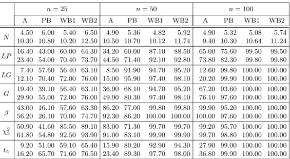
and the null hypothesis is simple, the simplifications in Remark 3.2 can be applied. Table 5 displays the results obtained for the type I error and the power for testing normality and Table 6 for testing GOF to the Laplace distribution. Similar conclusions to those given for Tables 1 and 2 can be also expressed in this case.
Table 5: (Heteroscedastic model) Percentage of rejections for the normality null hypothesis at the significance levels 5% (upper entry) and 10% (lower entry).
n= 25 n= 50 n= 100 A PB WB1 WB2 A PB WB1 WB2 A PB WB1 WB2 N 4.50 6.00 5.40 6.50 4.90 5.36 4.82 5.92 4.90 5.32 5.08 5.74 10.30 10.80 10.20 12.50 10.50 10.70 10.12 11.74 9.40 10.30 10.64 11.24 LP 16.40 43.00 60.00 64.30 34.20 60.00 87.10 88.50 65.00 75.60 99.50 99.50 23.40 54.00 70.40 73.70 44.50 71.40 92.10 92.80 73.80 82.30 99.80 99.80 LG 12.10 70.40 72.00 76.00 15.00 95.907.40 57.60 56.40 63.10 8.50 91.90 94.7097.40 95.2098.10 12.60 99.80 100.00 100.0020.20 99.90 100.00 100.00 G 19.40 39.10 56.40 63.10 36.90 68.10 94.70 95.20 67.20 93.60 100.00 100.00 29.90 55.00 72.00 76.00 49.90 80.30 97.40 98.10 76.10 97.60 100.00 100.00 β 43.00 16.10 57.60 63.30 86.20 77.00 99.80 99.80 99.90 95.20 100.00 100.00 56.20 26.10 70.00 74.70 92.30 86.20 100.00 100.00 100.00 97.60 100.00 100.00 χ2 3 50.90 41.60 85.50 89.10 83.00 71.30 99.70 99.70 99.20 95.70 100.00 100.00 61.80 54.80 92.50 93.90 91.00 83.10 99.90 99.90 99.70 98.80 100.00 100.00 t5 9.20 51.00 59.10 65.40 15.90 80.20 92.90 94.30 27.90 99.00 100.00 100.00 16.20 65.70 71.60 76.50 23.40 89.30 97.70 98.00 36.80 99.90 100.00 100.00
Table 6: (Heteroscedastic model) Percentage of rejections for the Laplace null hypothesis at the significance levels 5% (upper entry) and 10% (lower entry).
n= 25 n= 50 n= 100 A PB WB1 WB2 A PB WB1 WB2 A PB WB1 WB2 N 2.00 31.80 25.00 27.104.90 40.30 34.70 37.10 2.60 55.30 51.20 52.507.40 64.80 61.80 62.90 2.80 86.10 85.70 86.207.80 90.50 91.20 91.40 LP 2.106.80 10.004.60 8.003.70 4.609.60 3.007.30 11.505.70 4.009.20 10.204.40 3.607.80 9.104.40 8.404.00 4.409.00 LG 2.10 33.80 27.10 29.30 2.30 54.80 50.80 52.30 3.10 85.00 84.40 84.70 6.30 43.80 37.60 40.20 6.80 64.40 61.60 62.50 7.00 89.30 89.60 89.90 G 2.10 31.30 23.50 25.506.70 41.10 34.40 37.10 2.80 53.90 50.20 51.506.80 65.10 62.70 63.70 3.00 85.30 85.10 85.607.50 91.10 91.10 91.50 β 3.00 19.20 18.40 21.008.00 27.40 29.10 31.70 14.60 43.70 55.30 56.80 39.60 68.50 87.30 87.806.00 33.50 43.20 45.90 27.60 56.70 81.20 81.50 χ2 3 2.70 22.30 18.60 20.80 3.40 43.10 42.90 44.50 5.60 78.40 81.30 81.90 7.10 30.80 27.30 30.10 7.60 54.50 54.10 56.60 12.70 84.10 87.30 87.70 t5 2.90 30.60 22.80 24.50 3.90 56.80 53.20 53.90 4.60 84.30 83.90 84.30 6.30 41.50 33.70 38.00 6.50 66.70 64.30 65.20 9.40 90.20 90.40 90.70
5.3. Time consumed
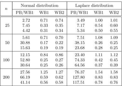
Table 7 compares the PB and the WB (with raw and centered multipliers) in terms of the required CPU time. This table shows the CPU time consumed in seconds to get a p-value for testing GOF for the normal and the Laplace distributions in the homoscedastic (for both single and composite null hypothesis) and the heteroscedastic models with sample sizes n= 25,50,100,200. Looking at this table it becomes evident that the WB is more efficient than the PB, in terms of the required computing time, specially for larger sample sizes. The difference in time when using the raw and the centered multipliers is rather small.
Table 7: CPU time consumed for the calculation of onep-value in seconds for testing normality and Laplace distribution for the homoscedastic model and composite null hypothesis (upper entry), the hetero-scedastic model (middle entry) and the homohetero-scedastic model and single null hypothesis (lower entry).
n Normal distribution Laplace distribution
PB/WB1 WB1 WB2 PB/WB1 WB1 WB2 2.72 0.71 0.74 3.49 1.00 1.01 25 7.45 0.33 0.35 7.17 0.54 0.60 4.42 0.31 0.34 5.34 0.50 0.55 5.61 0.71 0.70 7.51 1.08 1.09 50 30.88 0.17 0.22 38.15 0.26 0.25 15.63 0.19 0.19 23.68 0.28 0.25 12.15 0.84 0.86 23.40 1.11 1.12 100 52.80 0.25 0.27 74.33 0.42 0.45 30.64 0.25 0.26 64.56 0.37 0.39 27.56 1.25 1.27 76.37 1.54 1.58 200 66.19 0.59 0.62 127.80 0.83 0.83 41.14 0.56 0.58 117.51 0.78 0.76
The gain in computational efficiency of the WB over the PB stems from the fact that one does not have to re-estimate the parameters at each iteration, which slows down the process considerably. Note that in the WB the parameter θ, the regression functionm(.) and the conditional variance functionσ(·) are estimated only one time. For the WB approximation, once the set {mjk, 1≤j≤k≤n}is
6. CONCLUSIONS
This paper proposes a WB approximation for the null distribution of a test statistic for testing GOF to the error distribution in nonparametric mod-els. It provides a consistent estimator. The WB and the PB share this property. Nevertheless, from a computational point of view, the WB approximation is more efficient, in the sense of requiring less computation time. The numerical examples support these attributes. In addition, in cases were the asymptotic null distribu-tion does not depend on unknown quantities, the simuladistribu-tions carried out declare that, for small to moderate sample sizes, the WB provides a better fit than the asymptotic distribution.
To derive the results in this paper we considered certain estimators for the regression function and the conditional variance function. In addition, we assumed that the covariate was univariate. The results could be extended by considering other estimators (such as other local polynomial estimators) as well as covariates with higher dimension. The null distribution of other test statistics (for example, those based on the empirical CDF) could be similarly approximated.
7. APPENDIX
7.1. Assumptions
(A.2) The weight function ω satisfies (7.1) ω(t) =ω(−t), ∀t,
ω(t)≥0,∀t, andR
t4ω(t)dt <∞.
There is no restriction in assuming that the weight function ω(t) satisfies (7.1) because otherwise by definingω1(t) = 0.5{ω(t) +ω(−t)}, which satisfies (7.1), we
have that Tn,ω(ˆθ) =Tn,ω1(ˆθ).
(A.3) ε1, ..., εn are IID with E(εj4)<∞ and ε1, ..., εn and X1, ..., Xn are
independent.
Recall that by construction we have thatE(εj) = 0 and Var(εj) = 1.
(A.4) (i) X has a compact support S.
(ii) fX,m andσ are twice continuously differentiable onS.
(A.5) nh4n→0, nh2n/lnn→ ∞.
(A.6) K is a twice continuously differentiable symmetric pdf with com-pact support.
Assumptions (A.4)–(A.6) are mainly needed to guarantee the uniform con-sistency of the kernel estimators ˆfX(·), ˆm(·) and ˆσ(·) for fX(·), m(·) and σ(·),
respectively.
(A.7) The first partial derivatives R′(t;θ), I′(t;θ), R(r)(t;θ), I(r)(t;θ),
1≤r≤p, exist and are continuous functions ∀t∈R, ∀θ in an
open neighborhood of θ1. In addition, R′(t;θ), I′(t;θ), R(r)(t;θ), I(r)(t;θ), tR′(t;θ), tI′(t;θ), tR(r)(t;θ), tI(r)(t;θ), 1≤r ≤p, are
bounded by functions inL2(ω),∀θin an open neighborhood ofθ1.
The following assumption will be used for the maximum likelihood estima-tor of the parameter.
(A.9) The following functions exist∀θ in an open neighborhood ofθ1: ur(x;θ) = ∂θ∂r logf(x;θ) , u1,r(x;θ) = ∂ 2 ∂x∂θr logf(x;θ), u0,r,s(x;θ) = ∂2 ∂θr∂θslogf(x;θ) , u2,r(x;θ) = ∂ 3 ∂x2 ∂θr logf(x;θ), u1,r,s(x;θ) = ∂3 ∂x∂θr∂θs logf(x;θ) , and satisfy |u1,r(a1+a2x;θ)| ≤b1,r(x), with xb1,r(x), b1,r(x)∈L2(F) , |u0,r,s(a1+a2x;θ)| ≤b0,r,s(x)∈L2(F) , |u2,r(a1+a2x;θ)| ≤b2,r(x)∈L2(F) , |u1,r,s(a1+a2x;θ)| ≤b1,r,s(x)∈L2(F) ,
∀a1, a2, θsuch that|a1|,|a2−1|,|θ−θ1|≤δ, for some smallδ, 1≤r, s≤p.
In addition, the following expectations exist:
E
ur(ε;θ1)us(ε;θ1) ,
E
εu1,r(ε;θ1) ,
1≤r, s≤p.
The following assumption will be used for the method of moment estimator of the parameter, which assumes that under the null hypothesis, θ0 =g(µ0), for
some known function g= (g1, ..., gp)T,gr:Rk−1 →R, 1≤r ≤p:
(A.10) gr is twice continuously differentiable at a neighborhood of µF,
7.2. Proofs
We now sketch the proofs of the results stated in the previous sections, as well as some preliminary results. Along this sectionM denotes a generic positive constant taking many different values.
Lemma 7.1. Suppose that assumptions (A.3)–(A.6) hold, then
(a) 1nPn j=1(εj−εˆj)2 =op(1). (b) 1nPn j=1(ˆε2j −ε2j)2 =op(1). (c) 1nPn j=1(ˆε2j −1)2=Op(1). (d) 1nPn j=1εˆ2j =Op(1).
Proof: First, observe that under the considered assumptions (see, for example, Masry [16]) sup x∈S| ˆ m(x)−m(x)| = op(n−1/4), (7.2) sup x∈S| ˆ σ(x)−σ(x)| = op(n−1/4). (7.3)
The difference between the residuals and the errors can be written as follows
(7.4) εˆj−εj =εj σ(Xj)−σˆ(Xj) ˆ σ(Xj) + m(Xj)−mˆ(Xj) ˆ σ(Xj) .
The results in (a)–(d) follow from (7.2)–(7.4).
Lemma 7.2. Ifkθˆ−θ1k=op(1)and (A.7) holds, then
(a) kt{R′(t; ˆθ)−R′(t;θ1)}k2ω=op(1), kt{I′(t; ˆθ)−I′(t;θ1)}k2ω=op(1). (b) R k∇R(t; ˆθ)− ∇R(t;θ1)k2ω(t)dt=op(1), R k∇I(t; ˆθ)− ∇I(t;θ1)k2ω(t)dt=op(1). (c) kR(t; ˆθ)−R(t;θ1)k2ω =op(1), kI(t; ˆθ)−I(t;θ1)k2ω =op(1). (d) kt{R(t; ˆθ)−R(t;θ1)}k2ω =op(1), kt{I(t; ˆθ)−I(t;θ1)}k2ω =op(1).
Proof: (a) From (A.7)tR′(t;θ)∈L2(ω),∀θin a neighborhood ofθ1. Since ˆ
θ→P θ1, the integralR{R′(t; ˆθ)−R′(t;θ1)}2t2ω(t)dtis finite with probability
tend-ing to 1. Thus, ∀ǫ >0,∃M =M(ǫ)>0 such that (7.5)
Z
R\[−M,M]{
with probability tending to 1. tR′(t;θ) is a uniformly continuous function in [−M, M]×Bδ(θ1) =C, where Bδ(θ1) ={θ:kθ−θ1k ≤δ}. Thus, ∀ǫ >0, ∃ ρ= ρ(ǫ)>0 such that∀(ta, θa),(tb, θb)∈Csatisfyingk(ta, θa)−(tb, θb)k< ρ, we have
|t1R′(ta;θa)−t2R′(tb;θb)|< ǫ/ι, withι= R ω(t)dt. As a consequence (7.6) Z M −M{ R′(t; ˆθ)−R′(t;θ1)}2t2ω(t)dt < ǫ,
with probability tending to 1. Asǫis arbitrary, the result in (a) for the real part follows from (7.5) and (7.6). The proof for the imaginary part is parallel.
(b) The proof of this part is quite similar to that of part (a).
Parts (c) and (d) can be proven by applying the mean value theorem.
Proof of Theorem 2.1: W∗ can be expressed as W∗ =W1+W2+ 2W3,
whereW32≤W1W2,W1=k√1nPnj=1Z0(εj;t, θ1)ξjk2ω,W2=k√1nPnj=1{Z0(ˆεj;t,θˆ)
−Z0(εj;t, θ1)}ξjk2ω. From the results in [4],
sup
x |P∗{W1 ≤x} −P{W0≤x}| a.s.
−→0.
Thus, to show the result it suffices to see that W2 =op∗(1) in probability. With
this aim, observe that W2 can be expressed as W2=P4j=1Sj +Pj6=kSjk, with
Sjk2 ≤SjSk, 1≤j, k≤4. In the proof of Theorem 3.1 it is given the expression
ofSj and it is also proven thatSj =op∗(1) in probability, 1≤j≤4. This proves
the result.
Proof of Theorem 3.1: T2∗,n,ω(ˆθ) can be expressed as T2∗,n,ω(ˆθ) =D1+
D2+ 2D3, whereD1 =k√1nPnj=1Z2(εj;t, θ1)ξjk2ω,D2 =k√1nPjn=1{Z2(ˆεj;t,θˆ)−
Z2(εj;t, θ1)}ξjk2ω,D23 ≤D1D2. From the results in [4],
sup
x |
P∗{D1 ≤x} −P{T2≤x}|−→a.s. 0.
Thus, to show the result it suffices to see that D2 =op∗(1) in probability. With
this aim, observe that D2 can be expressed as
D2 = 10 X j=1 Sj + X k<j Sjk, with Sjk2 ≤SjSk, 1≤j, k≤10, S1 =k√1nPnj=1{cos(tεj)−cos(tεˆj)}ξjk2ω, S2 =k√1nPnj=1{sin(tεj)−sin(tεˆj)}ξjk2ω, S3 =k√1n{R(t; ˆθ)−R(t;θ1)}Pn j=1ξj k2ω,
S4=k√1n{I(t; ˆθ)−I(t;θ1)} Pn j=1ξj k2ω, S5=k√tnPjn=1{εˆjR(t; ˆθ)−εjR(t;θ1)}ξjk2ω, S6=k√tnPjn=1{εˆjI(t; ˆθ)−εjI(t;θ1)}ξjk2ω, S7=k2√tnPnj=1{(ˆε2j −1)R′(t; ˆθ)−(ε2j −1)R′(t;θ1)}ξjk2ω, S8=k2√tnPn j=1{(ˆε2j −1)I′(t; ˆθ)−(ε2j −1)I′(t;θ1)}ξjk2ω, S9=k√1nPnj=1{ψnT(ˆεj; ˆθ)∇R(t; ˆθ)−ψT1(εj;θ)∇R(t;θ1)}ξjk2ω, S10=k√1 n Pn j=1{ψTn(ˆεj; ˆθ)∇I(t; ˆθ)−ψ1T(εj;θ)∇I(t;θ1)}ξjk2ω.
We will show that Sj =op∗(1) in probability, 1≤j ≤10. By the mean value
theorem, S1 = 1 n n X j,k=1 ξjξk(εj−εˆj)(εk−εˆk) Z t2sin(t∼εj) sin(t∼εk)ω(t)dt,
where ∼εj=αjεj+ (1−αj)ˆεj, for someαj ∈(0,1). Then, from Lemma 7.1 (a),
E∗(S1)≤ 1 n n X j=1 (εj−εˆj)2 Z t2ω(t)dt=op(1),
which impliesS1 =op∗(1) in probability. Analogously,S2=op∗(1) in probability.
Since S3 = 1 √ n Pn j=1ξj 2
kR(t; ˆθ)−R(t;θ1)k2ω, the central limit theorem
and Lemma 7.2 (c) imply that S3 =op∗(1) in probability. Analogously, S4 = op∗(1) in probability.
Observe thatS5 =S51+S52+ 2S53, withS532 ≤S51S52,
S51= n1Pnj,k=1(ˆεj−εj)(ˆεk−εk)ξjξkktR(t; ˆθ)k2ω,
S52= n1Pnj,k=1εjεkξjξkkt{R(t; ˆθ)−R(t;θ1)}k2ω.
From Lemma 7.1 (a) and Assumption (A.2), it follows thatE∗(S51) =op(1) and
thusS51=op∗(1), in probability. From Lemma 7.2 (d), it follows thatE∗(S52) = op(1) and thusS52=op∗(1), in probability. Therefore,S5 =op∗(1), in probability.
Analogously,S6 =op∗(1), in probability.
Observe thatS7 =S71+S72+ 2S73, withS732 ≤S71S72, S71= 14n1 Pn
j,k=1(ˆε2j −1)(ˆε2k−1)ξjξkkt{R′(t; ˆθ)−R′(t;θ1)}k2ω,
S72= 14n1 Pn
j,k=1(ˆε2j −ε2j)(ˆε2k−εk2)ξjξkktR′(t;θ1)k2ω.
From Lemma 7.1 (c) and Lemma 7.2 (a), it follows thatE∗(S71) =op(1) and thus
From Lemma 7.1 (b) and (A.7), it follows that E∗(S72) =op(1) and thus
S72=op∗(1), in probability. Therefore, S7=op∗(1), in probability. Analogously, S8 =op∗(1), in probability.
Observe thatS9 =S91+S92+ 2S93, withS932 ≤S91S92,
S91=k√1nPnj=1{ψn(ˆεj; ˆθ)−ψ1(εj;θ1)}T∇R(t; ˆθ)ξjk2ω,
S92=k√1nPnj=1ψ1(εj;θ1)T{∇R(t; ˆθ)− ∇R(t;θ1)}ξjk2ω.
From (3.2) and (A.7), it follows that E∗(S91) =op(1) and thus S91=op∗(1), in
probability. From (A.1) and Lemma 7.2 (b), it follows thatE∗(S92) =op(1) and
thus S92=op∗(1), in probability. Therefore, S9=op∗(1), in probability.
Analo-gously, S10=op∗(1), in probability. This completes the proof.
Proof of Corollary 3.2: From Theorem 3.1 it follows that T∗
2,n,ω(ˆθ) =
Op∗(1) in probability. From Theorem 2 in [11],
Tn,ω(θ)
n P
−→κ >0. These two facts imply the result.
Lemma 7.3. Suppose that kθˆ−θ1k=op(1), for some θ1 ∈Θ, and that
assumptions (A.3)–(A.6), (A.9) hold, then
(a) 1nPn
j=1k∇logf(ˆεj; ˆθ)− ∇logf(εj;θ1)k2 =op(1).
(b) Aˆn,rs(ˆθ) =AF,rs(θ1) +op(1),1≤r, s≤p.
(c) ˆρ1(ˆθ) =ρ1,F(θ1) +op(1).
(d) ˆρ2(ˆθ) =ρ2,F(θ1) +op(1).
Proof: (a) From the mean value theorem and (A.9),
1 n Pn j=1 n ∂ ∂θr logf(ˆεj; ˆθ)− ∂ ∂θrlogf(εj;θ1) o2 = n1Pn j=1 n ∂2 ∂ε∂θr logf(˜εj; ˜θ)(ˆεj−εj) + Pp s=1 ∂ 2 ∂θr∂θslogf(˜εj; ˜θ)(ˆθs−θ1s) o2 ≤Sr,1+Sr,2+ 2Sr,3,
with Sr,23 ≤Sr,1Sr,2, ˜εj = (1−αj)ˆεj+αjεj, for some αj ∈(0,1), 1≤j≤n, ˜θ=
(1−α)ˆθ+αθ1, for someα∈(0,1), Sr,1 = kθˆ−θ1k2 1 n n X j=1 p X s=1 b20,r,s(εj) and Sr,2 = 1 n n X j=1 b21,r(εj)(ˆεj−εj) =op(1).
From (A.9), (7.2)–(7.4), it follows that Sr,1 =op(1), Sr,2 =op(1), 1≤r≤p.
This proves (a).
The proof of parts (b)–(d) follows similar steps to that of part (a).
Proof of Theorem 4.1: Observe that 1nPn
j=1kψ1n(ˆεj; ˆθ)−ψ(εj;θ1)k2 ≤ D1+D2+D3+D4, withD24 ≤ P j6=kDjDk, D1 = 1 n n X j=1 kAˆn(ˆθ)−1∇logf(ˆεj; ˆθ)−AF(θ1)−1∇logf(εj;θ1)k2, D2 = 1 n n X j=1 kεˆjρˆ1(ˆθ)−εjρF,1(θ1)k2, D3 = 1 n n X j=1 kεˆ 2 j −1 2 ρ2ˆ (ˆθ)− ε2 j −1 2 ρF,2(θ1)k 2.
By using the results in Lemmas 7.1 and 7.3 one obtain Dj =op(1), 1≤j≤3,
and hence the result.
Proof of Theorem 4.2: From (7.2)–(7.4), 1 √n n X j=1 ˆ εsj = √1 n n X j=1 εsj+√1 n n X j=1 εsj−1m(Xj)−mˆ(Xj) ˆ σ(Xj) (7.7) + √1 n n X j=1 εsjσ(Xj)−σˆ(Xj) ˆ σ(Xj) +op(1).
Taking into account the following facts
(m.1) supx∈S ˆ m(x)−m(x) ˆ σ(x) − ˆ m(x)−m(x) σ(x) =op(n −1/2), (m.2) supx∈S mˆ(x)−m(x)− 1 nfX(x) Pnv k=1Khn(x−Xk)σ(Xk)εk =op(n−1/2), it follows that 1 √ n n X j=1 εsj−1m(Xj)−mˆ(Xj) ˆ σ(Xj) = = −1 n√n n X j,k=1 εsj−1εk σ(Xk) fX(Xj)σ(Xj) Khn(Xj −Xk) +op(1).
Now, by using projections, we get (see, for example, the proof of Theorem 2 in [18] for a similar development)
(7.8) √1 n n X j=1 εsj−1m(Xj)−mˆ(Xj) ˆ σ(Xj) =−µF,s−1 1 √ n n X j=1 εj+op(1).
Next we deal with the third term in the right-hand side of (7.7). Taking into account the following facts
(s.1) supx∈S ˆ σ(x)−σ(x) ˆ σ(x) − ˆ σ(x)−σ(x) σ(x) =op(n −1/2), (s.2) supx∈S σˆ(x)−σ(x)− ˆ σ2 (x)−σ2 (x) 2σ(x) =op(n −1/2), (s.3) supx∈S σˆ 2(x)−σ2(x)− 1 nfX(x) Pn j=1Khn(Xj−x) ·h{Yj−m(x)}2−σ2(x) i =op(n −1/2), it follows that 1 √ n n X j=1 εsjσ(Xj)−σˆ(Xj) ˆ σ(Xj) = = 1 2n√n n X j,k=1 εsj 1 fX(Xj)σ2(Xj) Khn(Xj−Xk) σ2(Xj)− {Yk−m(Xj)}2+op(1).
Now, by using projections, we get (see, for example, the proof of Lemma 11 in [19] for a similar development)
(7.9) √1 n n X j=1 εsjσ(Xj)−ˆσ(Xj) ˆ σ(Xj) =−µF,s 2 1 √ n n X j=1 (ε2j −1) +op(1).
The result follows from (7.7)–(7.9).
Proof of Theorem 4.3: Notice that ˆ µs−µF,s= 1 n n X j=1 (ˆεsj−εsj) + 1 n n X j=1 (εsj−µF,s).
From (7.2)–(7.4), the first term in the right-hand side of the above equality is
op(1); from the SLLN, the second term in the right-hand side of the above equality
is o(1) a.s. Therefore ˆµs−µF,s=op(1), 2≤s≤k. The result follows from this
fact and (A.10).
ACKNOWLEDGMENTS
The authors thank the anonymous referee and the AE for their helpful sug-gestions and constructive comments. G.I. Rivas-Mart´ınez acknowledges financial support from Fundaci´on Carolina, Universidad Nacional de Asunci´on and Uni-versidad de Sevilla. M.D. Jim´enez-Gamero acknowledges financial support from grant MTM2014-55966-P of the Spanish Ministry of Economy and Competitive-ness, and grant MTM2017-89422-P of the Spanish Ministry of Economy, Industry and Competitiveness, ERDF support included.
REFERENCES
[1] Bickel, P.J.andDoksum, K.A.(2001).Mathematical Statistics, Prentice Hall, New Jersey.
[2] Burke, M.D.(2000). Multivariate tests-of-fit and uniform confidence bands us-ing a weighted bootstrap,Statistics & Probability Letters,46, 13–20.
[3] de U˜na- ´Alvarez, J. (2013). Comments on: An updated review of Goodness-of-Fit tests for regression models,Test,22, 414–418.
[4] Dehling, H.and Mikosch, T.(1994). Random quadratic forms and the boot-strap forU-statistics,Journal of Multivariate Analysis,51, 392–413.
[5] Feller, W.(1971). An Introduction to Probability Theory and its Applications, Vol. 2, Wiley, New York.
[6] Heuchenne, C. and Van Keilegom, I. (2010). Goodness of fit tests for the error distribution in nonparametric regression,Computational Statistics & Data Analysis,54, 1942–1951.
[7] Epps, T.W.(2005). Tests for location-scale families based on the empirical cha-racteristic function,Metrika,62, 99–114.
[8] Epps, T.W. and Pulley, L.B.(1983). A test for normality based on the em-pirical characteristics function,Biometrika,70, 723–726.
[9] Gonz´alez-Manteiga, W. and Crujeiras, R. (2013). An updated review of Goodness-of-Fit tests for regression models,Test,22, 361–411.
[10] Huˇskov´a, M.andJanssen, P.(1993). Consistency of the generalized bootstrap for degenerateU-statistics,The Annals of Statistics,21, 1811–1823.
[11] Huˇskov´a, M. and Meintanis, S.G. (2010). Test for the error distribution in nonparametric possiby heteroscedatic regression models,Test,19, 92–112. [12] Jim´enez-Gamero, M.D.; Alba-Fern´andez, V.; Mu˜noz-Garc´ıa, J. and
Chalco-Cano, Y. (2009). Goodness-of-fit tests based on empirical characte-ristics functions,Computational Statistics & Data Analysis,53, 3957–3971. [13] Jim´enez-Gamero, M.D. (2013). Comments on: An updated review of
Goodness-of-Fit tests for regression models,Test,22, 412–413.
[14] Jim´enez-Gamero, M.D.andKim, H-M.(2015). Fast goodness-of-fit test based on the characteristic function, Computational Statistics & Data Analysis, 89, 172–191.
[15] Kojadinovic, I. and Yan, J. (2012). Goodness-of-fit testing based on a weighted bootstrap: A fast sample alternative to the parametric bootstrap, The Canadian Journal of Statistics,40, 480–500.
[16] Masry, E.(1996). Multivariate local polynomial regression for time series: uni-form strong consistency and rates,Journal of Time Series Analysis,17, 571–600. [17] Neumeyer, N.; Dette, H. and Nagel, E-R. (2006). Bootstrap test for the error distribution in linear and nonparametric regression models, Australian & New Zealand Journal of Statistics,48, 129–156.
[18] Pardo-Fern´andez, J.C.; Jim´enez-Gamero, M.D. and El Ghouch, A.
(2015). A nonparametric ANOVA-type test for regression curves based on char-acteristic functions,Scandinavian Journal of Statistics,42, 197–213.
[19] Pardo-Fern´andez, J.C.; Jim´enez-Gamero, M.D. and El Ghouch, A.
(2015). Tests for the equality of conditional variance functions in nonparametric regression,Electronic Journal of Statistics,9, 1826–1851.
[20] R Core Team(2015). R: A language and environment for statistical computing. R Foundation for Statistical Computing, URL:http://www.R-project.org/, Vienna,
Austria.
[21] Sperlich, S.(2013). Comments on: An updated review of Goodness-of-Fit tests for regression models,Test,22, 419–427.
[22] White, H. (1982). Maximum likelihood estimation of misspecified models, Econometrica,50, 1–25.
[23] Zhu, LX. (2005). Lecture Notes in Statistics. Nonparametric Monte Carlo test and their applications, Springer, Berlin.