Population dynamic of early stages of
Caligus rogercresseyi
in an embayment used for
intensive salmon farms in Chilean inland seas
Carlos Molinet
a,b,c,⁎
, Mario Cáceres
d, Maria Teresa Gonzalez
f, Juan Carvajal
e, Gladys Asencio
e,
Manuel Díaz
a, Patricio Díaz
a, Maria Teresa Castro
e, José Codjambassis
aa
Instituto de Acuicultura, Universidad Austral de Chile, Los Pinos s/n, Balneario Pelluco, Puerto Montt, Chile b
Centro Trapananda, Universidad Austral de Chile, Portales 73 Coyhaique, Chile c
CIEN Austral, Los Pimientos 4369, Puerto Montt, Chile d
Universidad de Valparaíso, Borgoño 16344, Montemar, Viña del Mar, Chile
eCentro I-mar, Universidad de Los Lagos, Camino a Chinquihue Km 6, Puerto Montt, Chile f
Instituto de Investigaciones Oceanólogicas, Universidad de Antofagasta, Casilla 170, Antofagasta, Chile
a b s t r a c t
a r t i c l e i n f o
Article history: Received 28 June 2010
Received in revised form 5 December 2010 Accepted 7 December 2010
Available online 13 December 2010 Keywords: Sealouse Pest management Larvae Ovigerous female Circulation pattern Salmon farm
Around the world several strategies for the management and control of sea lice infestations have been implemented. In Chile where the salmon harvest is significantly higher than other countries and where salmonids are not endemic species, information concerning how farm locations and local oceanographic conditions interact in regulating the dispersal of parasites and their impact on farmed and nativefish populations is required urgently. In this work we studied the spatial and temporal dynamics of the early stages ofCaligus rogercresseyiin a semi-enclosed area where eight salmon farms are located in southern Chile. Plankton samples were collected in three modes (fortnightly, diurnal and semidiurnal spatial), which were complemented by studying circulation patterns inside the bay. Simultaneously, records of ovigerous femaleC. rogercresseyiperfish, treatments for caligids, biomass, and the average weight offish were obtained from salmon farms in the study area. Our results suggest that the population dynamics of the early stages ofC. rogercresseyiis strongly associated to salmon farm, which could be magnified by the effect of the local circulation pattern. In this context it seems unlikely to control, through current caligid treatments, the caligid pest in this semi-enclosed area without a drastic decrease of salmon biomass inside the bay. The salmon farms should be located distant enough between them to minimize risks and maximizes benefits to all concerned parties.
© 2010 Elsevier B.V. All rights reserved.
1. Introduction
Around the world several management strategies for the control of sea lice infestations have been implemented (Andersen and Kvenseth, 2000; Bron et al., 1993; Costello, 2009; Kvenseth and Kvenseth, 2000). According to Revie et al. (2009) when large numbers of farmed salmon are introduced to the marine environment within open net cage salmon farms, it is virtually to impossible to avoid (1) the infection of farmedfish, all of which go into the pens as clean smolts, and (2) the subsequent infection of wildfish that are found in the vicinity (“infectivefield”) of the installation. Therefore, management strategies must be designed taking into account the regional, biological and environmental factors that influence the severity of sea lice infections (Brooks, 2009; Murray and Peeler, 2005; Penston and Davies, 2009; Revie et al., 2009).
In Chile where the salmon harvest is orders of magnitude higher than in other countries, and where salmonids are not endemic species, urgent attention is required in order to understand how farm location and water current patterns interact in regulating the dispersal of parasites, and their population dynamics (Buschmann et al., 2009).
Caligus rogercresseyiBoxshall and Bravo (2000) is the dominant sea louse parasite affecting the salmon and trout industry in Southern Chile (González and Carvajal, 2003). The parasite was transmitted to the farmed fish by the native rock cod Eleginops maclovinus and Odonthestes regia(Carvajal et al., 1998). These were the most common wild hosts of C. rogercresseyi, C. teres, C. cheilodactylus and Lepeophtheirus mugiloides(Carvajal et al., 1998; Revie et al., 2009). Despite the impact of the caligid parasite on the salmon industry in Chile (Bravo, 2003; Johnson et al., 2004) and the likelihood that transmission between populations occurs during the planktonic stages, there is no published account of the larval ecology of C. rogercresseyi. Also, increasing economic losses due to parasite infestations have led to the increased use of chemicals to control the caligids (Bravo et al., 2008; Pino-Marambio et al., 2007).
Laboratory studies have shown that C. rogercresseyi has eight developmental stages: three planktonic andfive parasitic (González
⁎ Corresponding author. Instituto de Acuicultura, Universidad Austral de Chile, Los
Pinos s/n, Balneario Pelluco, Puerto Montt, Chile. Tel.: + 56 65 277126; fax: + 56 65 255583.
E-mail address:cmolinet@uach.cl(C. Molinet).
0044-8486/$–see front matter © 2010 Elsevier B.V. All rights reserved.
doi:10.1016/j.aquaculture.2010.12.010
Contents lists available atScienceDirect
Aquaculture
and Carvajal, 2003). The planktonic stages are non-feeding and comprise two nauplii and one copepodid stage. It is during the latter stage that infection occurs. The planktonic stages begin with thefirst nauplius (average length = 425μm), 3 days later the larvae trans-forms into the second nauplius (average length = 463μm). Once transformed into the copepodid stage it settles on the host, holding on with its hooked pair of antennae (González, 2006). Depending on seawater temperature, as observed inLepeophtheirus salmonis(Stien et al., 2005), the lifespan of the planktonic stages vary, and can last between 5 and 9 days in the laboratory, after which the copepodids are ready to settle (Farias, 2005; González, 2006). The parasitic stage begins withfirst chalimus, develops through to the fourth chalimus,
finally ending in the adult males and females. Attachment is stronger after thefifth day when the accumulated temperature is over the 50th degree—days of effective temperature (González and Carvajal, 2003). During the 5 to 9 days spent in the plankton, significant transport and dispersion within surface currents are possible. Over this period of time, the transmission risks to other populations will depend on the rate of dispersion and the direction of transport from the point of origin, as has been observed for the larvae of the sea louse of L. salmonis(Kroger, 1838;Amundrud and Murray, 2009).
To estimate the transmission potential of sea lice, it is essential to understand where the local circulation may transport the planktonic stages of the lice. Epidemiological studies have found thatL. salmonis abundance onfish farms is related to local current speeds and the sea loch
flushing times, highlighting the importance of the physical circulation (among other factors) to the infection processes (Amundrud and Murray, 2009; Genna et al., 2005). Planktonic stages of sea lice are vulnerable to low salinities (Stien et al., 2005) and have been described as essentially passive, with a limited vertical swimming ability that allows them to remain near the surface (Bron et al., 1993). Also, laboratory experiments have shown that the copepodids ofL. salmonisare strongly phototactic (Genna et al., 2005), confirming thefield observations ofHeuch et al. (1995). These authors observed that nauplii exhibited only small differences in depth between night and day while copepodid distribution appeared to be controlled by light intensity. These results suggest the
presence of aggregations of larvae in surface layers during daylight; however, despite intensive sampling along coasts of several countries, pelagic swarms of copepodids have not been found (Penston et al., 2002). The objective of this research was to study the spatial and temporal dynamics of the early stages ofC. rogercresseyiassociated with the abundance ofC. rogercresseyiovigerous females in a semi-enclosed area where 8 farms are located in southern Chile, in order to provide a more comprehensive source of information for developing management strategies for salmon farming.
2. Methodology 2.1. Study area
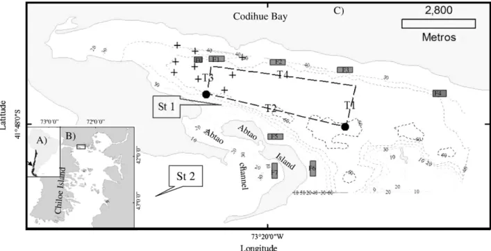
The study was carried out in Codihue Bay (41°48′S and 73°20′W) at the northwestern end of Patagonian inland sea. Codihue Bay has an east– west orientation, a maximum depth of 60 m, and opens to the east. The bay is ~ 12 km long, and 3–4 km wide, and is connected to Chacao Channel through the Abtao Channel (Fig. 1). The water column is relatively homogeneous (around 32 psu) and temperatures range between 9 °C and 15 °C at the surface during winter and summer, respectively. Eight salmon farms were operating during the period of the present study (named F0 to F7); F0 being an experimental farm (Fig. 1).
2.2. Data collection
In order to study larval spatial and temporal variability in C. rogercresseyiwithin the study area and their relationship with environ-mental variables, three modes of plankton sampling were carried out: i) fortnightly, ii) diurnal, and iii) spatial-semidiurnal, which were com-plemented with temperature and salinity records, and a characterization of sea current patterns.
C. rogercresseyi larvae were sampled by towing plankton nets (0.6 m in diameter × 1.5 m in length; with 150μm mesh size) from a 10–15-meter boat. The towed distance was estimated from the boat
Fig. 1.A) Region of South America (black arrow) where the study took place in Southern Chile (Chile is highlighted in dark colour). B) Chilean inland sea in northwest Patagonia, the
position of Codihue bay is denoted by a rectangle. C) Thefine scale representation shows the 0, 10, 20, 30, 40, 50, and 60-meter isobaths (gray dotted lines). Also displayed are the
sample stations of mode 1 (annual) (St 1, inside the bay, and St 2 outside the bay); the track followed during the 24 h of ADCP sample collection (dark gray dotted which formed an irregular polygon) and the four transect studied (T1 = transect 1, T2 = transect 2, T3 = transect 3, and T4 = transect 4). Black dots at the ends of transect 2 shows the CTD east and west stations. Crosses show the nine sample stations of mode 3 (spatial semidiurnal). Gray rectangles show the location of farms which producing salmon during the study period.
velocity (2 knots, controlled by a GPS Garmin), and time of tow, which ranged from 3 to 5 min depending on the sample mode.
2.2.1. Mode 1
Fortnightly samples were collected from July 2008 to June 2009 at one inside station and one outside station of Codihue Bay (Stations 1 and 2 in
Fig. 1). Within two strata (surface and 10–15-meter depth) three samples
were taken by towing plankton nets for 5 min at a speed of ~ 2 knots. Over the same period, ovigerous females ofC. rogercresseyiwere sampled from netpen-reared rainbow trout (Oncorhynchus mykiss) and Atlantic salmon (Salmo salar) (10fish per cage) from eight farms in Codihue Bay. In addition, monthly values of salmon biomass from the same farms were obtained. Using the averaged weight offishes sampled and the total biomass we estimated the number offishes.
Surface, Station 1 0 20 40 60 80 100 Jul-08 Jul-08
Aug-08 Sep-08 Oct-08 Nov-08 Jan-09 Feb-09 Apr-09 Apr-09 May-09 Jun-09
Date (Month-year)
NI NII COP 15 m, Station 1 0 2 4 6 8 10 Jul-08 Jul-08Aug-08 Sep-08 Oct-08 Nov-08 Jan-09 Feb-09 Apr-09 Apr-09 May-09 Jun-09
Date (Month-year)
NI NII COP Surface, Station 2 0 2 4 6 8 10Jul-08 Jul-08 Aug-08 Sep-08 Oct-08 Nov-08 Jan-09 Feb-09 Apr-09 Apr-09 May-09
Date (Month-year) NI NII COP 15 m, Station 2 0 2 4 6 8 10
Jul-08 Jul-08 Aug-08 Sep-08 Oct-08 Nov-08 Jan-09 Feb-09 Apr-09 Apr-09 May-09
Date (Month-year)
Larval abundance
Larval abundance
Larval abundance
Larval abundance
NI NII COPA)
B)
C)
D)
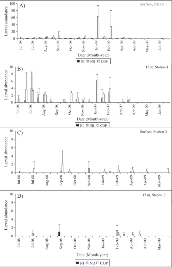
Fig. 2.Caligus rogercresseyilarval abundance (nauplii II and copepodids) inside Codihue bay (at the surface (A) and 15-meter depth (B)); and outside Codihue bay (at the surface (C) and 15-meter depth (D)).
2.2.2. Mode 2
Diurnal sampling (24 h) was undertaken on July 29/30, 2008 (winter survey); April 24/25, 2009 (autumn survey); and November 16/17, 2009 (spring survey). Three samples were collected simultaneously at the surface, 10–15 m, and 20–25 m by plankton nets towed for 5 min, every 3–3.5 h at station 1, inside Codihue Bay (Fig. 1C). Temperature and salinity were recorded at the beginning and end of the tows with a Seabird SBE-19 conductivity–temperature–depth (CTD) recorder. During the autumn survey, current velocity profiles were recorded with a broadband 300 kHz RD-Instruments acoustic Doppler current profiler (ADCP) across four transects: 1) eastern (across-bay), 2) southern (along-bay), 3) western (across-bay), and 4) northern (along-bay (Fig. 2A)). These transects were sampled 14 times during a 24-hour period. The ADCP was towed on a 1.2-meter long catamaran positioned on the starboard side of the R/V Monica VI at speeds of between 2.0 and 2.5 m s−1. Velocity profiles with a vertical
resolution of 2 m and ping rates of ~1 Hz were averaged every 60 s, yielding a spatial resolution of 120–150 m. The ADCP compass was calibrated using Global Positioning System (GPS) navigation data. 2.2.3. Mode 3
Spatial sampling (a semidiurnal tidal cycle) was undertaken on December 4th 2008, using a spatial grid of nine stations inside Codihue
Bay where two plankton nets were towed for a period of 3 min at 2 knots at each station. Surface samples were collected every 3 h and temperature and salinity were recorded in a DST logger attached to each net. In addition, before the plankton sampling began, ten drifters were deployed around station 1 (Fig. 1C) at the surface (five drifters) and at a depth of 20 m (five drifters). The movement of these drifters was then followed over the 12 h of the semidiurnal cycle.
Table 1
Results from the sequential deviance analysis for the response variable ovigerous
female ofC. rogercresseyibetween May 2008 and June 2009. Predictive variables were:
month, farm, total biomass and total number offish in salmon farms of Codihue bay,
host species,fish weight and chemical treatment for caligids.
Degrees of freedom Deviance residual Df. residual Deviance P (Nχ2 ) Null 1454 3387 Month 13 546.5 1441 2840 0.00001 Farm 8 295.6 1434 2545 0.00001 Biomass 1 28.1 1433 2517 0.00001 Host species 1 34.9 1432 2482 0.00001 Meanfish weight 1 0.2 1431 2481 0.6 Number offishes 1 0.3 1430 2481 0.6 Treatment 3 356.9 1427 2124 0.00001 0 2000 4000 6000 8000 10000 12000 14000 16000 18000 20000
2008/May 2008/Jul 2008/Aug 2008/Oct 2008/Dec 2009/Feb 2009/Apr 2009/Jun 2009/Aug 2009/Oct 2009/Dec 2010/Feb 2010/Apr 2010/Jun
Biomass (Tons.)
Thousands of fishes
Thousands of Ovigerous female
0 500 1000 1500 2000 2500 3000 3500
Fish weigth (gr)
Biomass
Nº of Fishes
Nº Ov. Female
Fish weight
0 5 10 15 20 25 30 35 40 2008/Jul
2008/Aug 2008/Sep 2008/Oct 2008/Nov 2008/Dec 2009/Jan 2009/Feb 2009/Mar 2009/Apr 2009/May 2009/Jun 2009/Jul
Date (month)
Larvae/ 87 m
3 0 2000 4000 6000 8000 10000 12000 14000 16000 18000 20000Thousands of
Ovigerous female
COP
NII
Ov. Female
A)
B)
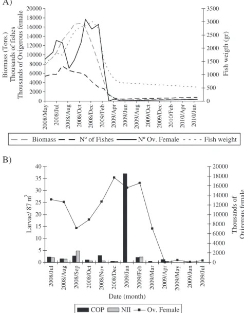
Fig. 3.A) Estimated ovigerous female ofC. rogercresseyibetween May 2008 and June 2010 and the variation of salmon biomass, number offish, host species,fish weight and chemical
2.3. Data analysis
To select explanatory variables for abundance ofC. rogercressseyi, nauplii and copepodids during our three sample modes of data collection and for abundance of ovigerous female in the study area we applied generalized linear models, GLM (McCullagh and Nelder, 1989), assuming a Poisson distribution for errors of the untransformed
response variable. To avoid collinearity among the variables, they were tested one at a time, choosing the one providing the bestfit according to Akaike's information criterion (AIC). A deviance analysis was used to evaluate the relative contribution of each variable in explaining the variability in the response variable. The significance of each explanatory variable was determined using aχ2test (Venables and Ripley, 1998).
Larval abundance of C. rogercresseyi and density of the surface seawater obtained from the 9 stations of Mode 3, and track drifters were referenced and deployed in a Geographic Information System (SIG) utilizing Arc Gis 9.3.
CTD data obtained during Modes 2 and 3 were processed using the manufacturer's software, and the processed data were used to produce density profiles using Surfer 7.0 software (Golden Software).
Current velocity data were processed following the approach of
Valle-Levinson and Atkinson (1999). After the heading correction was applied, the data were rotated anti-clockwise to an along- (vflow) and across- (uflow) channel coordinate system. These angles were oriented in the direction of greatest variability in the tidal currents and of weakest across-channel tidal flows. Semidiurnal (M2) and
diurnal (K1) constituents were separated from the subtidal signal of
the observed flow components using sinusoidal least squares regression analysis (Lwiza et al., 1991).
Nauplii II, winter
-25 -20 -15 -10 -5 30.5 30.7 30.9 31.1 31.3 31.5
Copepodid, winter
-25 -20 -15 -10 -5Depth (m)
Depth (m)
Depth (m)
Day of August 2008
Density (Kg/m ), winter
-25 -20 -15 -10 -5 3Day of April 2009
Density (Kg/m ), autumn -25 -20 -15 -10 -5 3Day of November 2009
Density (Kg/m ), spring
-25 -20 -15 -10 -5 3 19.5 19.7 19.9 20.1 20.3Copepodid, spring
-25 -20 -15 -10 -5 24.5 24.7 24.9 25.1 25.3Copepodid, autumn
-25 -20 -15 -10 -5Hei
g
ht
tid
e
Nauplii II, autumn
-25 -20 -15 -10 -5 30.5 30.7 30.9 31.1 31.3 31.5 30.5 30.7 30.9 31.1 31.3 24.5 24.7 24.9 25.1 25.3 19.5 19.7 19.9 20.1 20.3 24.5 24.7 24.9 25.1 25.3 19. 5 19.7 19.9 20. 1 20.3
Nauplii II, spring
-25 -20 -15 -10 -5 0 to 0.1 0.2 to 1 1.1 to 5 5.1 to 10 10.1 to 16
Fig. 4.Results of the three diurnal samples (mode 2) carried out during winter 2008, autumn and spring 2009. Gray zones show dark (night) hours. Thefirst three panels show copepodids abundance during the 24-hour sampling. The second three panels show nauplii II abundance during the 24-hour sampling. The third three panels show density of the water column during the sample period. The three waves showed at the base of the panels show tide variability during the sample period.
Table 2
Results from the sequential deviance analysis for the response variable larval
abundance ofC. rogercresseyiin mode 1 of sample collection (fortnightly). Predictive
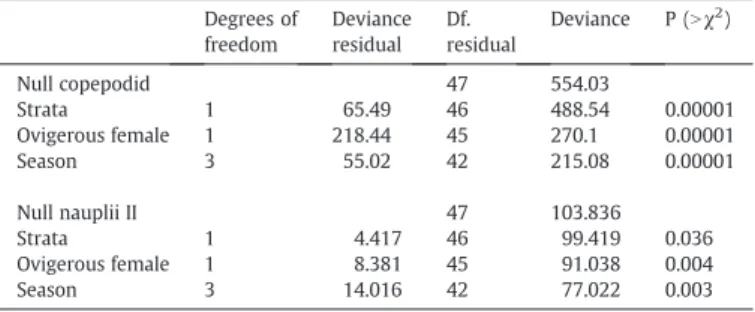
variables were: strata, ovigerous female, and season. Degrees of freedom Deviance residual Df. residual Deviance P (Nχ2 ) Null copepodid 47 554.03 Strata 1 65.49 46 488.54 0.00001 Ovigerous female 1 218.44 45 270.1 0.00001 Season 3 55.02 42 215.08 0.00001 Null nauplii II 47 103.836 Strata 1 4.417 46 99.419 0.036 Ovigerous female 1 8.381 45 91.038 0.004 Season 3 14.016 42 77.022 0.003
3. Results
3.1. Mode 1: annual variation
The early stages ofC. rogercresseyiwere more frequent inside than outside of Codihue bay with the largest abundance of copepodids (90 copepodids per 87 m3) occurring during the summer months at the
surface (Fig. 2A). Three apparent peaks of larval abundances were observed inside the bay (during winter, spring and summer) in subsurface samples where nauplii II and copepodids exhibited similar magnitudes of abundance (Fig. 2B). The abundance of nauplii II ranged from 1 to 10 larvae × 87 m3, while nauplii I were rare during
the entire study period in all of sampling modes. All the early stages of C. rogercresseyiwere scarce at the station outside the bay throughout
the study period, although it was observed higher larval abundance at the surface, (Fig. 2C) than at the subsurface samples (Fig. 2D).
Intensive salmon farming production occurred between April 2008 and March 2009 at the eight farms within the study area, reaching around 18,000 t of salmon (S. salarandO. mykiss), (around 6 million offish) (Fig. 3A). Between March 2009 and July 2009 onlyO. mykiss was farmed within the study area, with an average production of 1 t. per month. Taking into account the biomass of salmon in the farms, the abundance of ovigerous females inside the bay was estimated to vary from 200 individuals in autumn 2009 up to 18 million individuals during spring–summer 2009 (Fig. 3A). The period of maximum ovigerous female abundance was coincident with maximum abun-dance of copepodids, but not with nauplii II abunabun-dances (Fig. 3B).
According to the GLM analysis, month (June 2008, November 2008, and May 2009), treatment (no treatment and deltamethrin), and farm (Farm F0, F3 and F4) were the most important explanatory variables of ovigerous female abundances (explaining 16%, 13% and 9% of total deviance, respectively), while farmed species and total biomass explained less than 1% of total variability. Individual mean
fish weight and the total number of farmedfish in the bay did not contribute to the explanation of the ovigerous females' variability (pN0.05,Table 1).
Annual variability of copepodids was significantly explained by the number of ovigerous females (40% of deviance), depth strata (12% of deviance) and season (10% of deviance). Annual variability of nauplii II was also explained by the same variables, however these accounted for only 25% of the total deviance (Table 2).
3.2. Mode 2: diurnal variation
During the three diurnal surveys carried out between 2008 and 2009 only nauplii II and copepodid stages were found. As observed during Mode 1, copepodids were more frequent than stage II nauplii. Table 3
Results from the sequential deviance analysis for the response variable larval
abundance ofC. rogercresseyiin mode 2 of sample collection (diurnal). Predictive
variables were: season, day period, tide, strata, and density water. Degrees of freedom Deviance residual Df. residual Deviance P (Nχ2 ) Null copepodid 69 76.151 Season 2 6.146 67 70.006 0.046 Day period 1 2.562 64 59.51 0.109 Tide 1 0.559 63 58.95 0.454 Strata 2 7.935 65 62.071 0.019 Density 1 0.143 62 58.807 0.705 Null nauplii II 69 168.468 Season 2 62.875 67 105.593 2.22E−14
Day period 1 27.36 66 78.232 1.69E−07
Tide 1 16.64 65 61.593 4.52E−05
Strata 2 4.861 63 56.732 0.088
Density 1 9.632 64 51.96 0.002
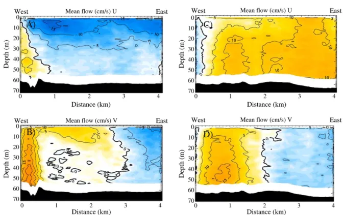
Fig. 5.Vertical contours of the residualflow in transects 2 and 4 for both U andVcomponents;Ucomponent are positive (yellow) toward the east, and negative (blue) toward the
west. ComponentVis positive (yellow) toward the north, and negative (blue) toward the south. White band close to the bottom shows data not considered for analysis because of
Nauplii II were more abundant during the winter survey, but this stage was scarce during the spring survey and was not recorded during the autumn survey (Fig. 4). Copepodid abundance was significantly affected by the season of the year and depth strata, exhibiting their highest abundance during the winter survey and in the surface samples (pb0.05), while tide and period of the day did not have a significant effect on copepodid abundances (Table 3). Nauplii II abundances were significantly explained by the variables season (highest abundance was observed during winter), period of the day (higher abundance during the day), tide (higher abundance during
flood tide), and water density (higher abundance with lower density) (pb0.05,Table 3,Fig. 4).
Vertical contours of residual flow from U (east–west) current components for transects 2 (Fig. 5A) showed a dominantflow toward the west for almost the entire water column, except for a narrow band at the western end of both transects. This band could be explained by the effect of the dominantflood tide current emanating from the Abtao Channel, which causes a convergence of the flow in the transitional area for both current directions. Across transect 4 this situation was reversed and the dominantflow was in an easterly direction within a narrow vertical bandflowing towards the west (Fig. 5C), suggesting that the current from the Abtao channel was divided on the north side of the bay promoting a divergence zone.
For theV(north–south) component offlow (Fig. 5B and D), the vertical band of positive flow (towards the north) on the left of transect 2 suggested an effect of theflood current from the Abtao Channel, as was observed for transect 4. In this case the portion of the
column water affected was wider than that observed in the U component, which suggests the presence of a gyre moving in a clockwise direction in the residualflow.
Vectorial residualflows at the two selected depths exhibited the tendency of theflow to rotate clockwise in the surface layer, and at a depth of 45 m. However part of the bottomflow (45 m) seemed to leave the bay moving eastwards (Fig. 6A), following the orientation of the submarine valley (Fig. 1). The dominantflow towards the north from the Abtao Channel was more clearly observed in deeper layers than at the surface, as demonstrated by the vertical contours.
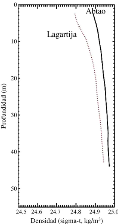
Vertical density profiles showed slight stratification and the observed density of the water column was slightly higher in the western CTD station (close to Abtao Channel) than in the eastern CTD station (close to Lagartija Island) (Fig. 7).
3.3. Mode 3: spatial variation
Spatial distribution of copepodids and nauplii II larvae was heterogeneous during the 12 h sampling period. Nauplii II ranged from 1 to 12 larvae per 34 m3(median = 0), while copepodids ranged
from 1 to 4 larvae per 34 m3 (median = 0). Both copepodids and
nauplii II were more abundant in thefirst sample which seemed to be associated with densityfields and theflood tide (Fig. 8). During the ebb tide larvae were more abundant towards the mouth of the bay, and in thefinal sample of the afternoon larvae were rare (Fig. 8). Drifters deployed at 20 m exhibited a larger displacement than surface drifters, although none of them moved more than 2 km inside
Fig. 6.A) Velocity vectors of the residualflow obtained with ADCP profiles at 1-meter and 45-meter depth (cm/s, without decimals). B) Flow direction and displacement of drifters at the surface and at the 20 m.
the bay (Fig. 6B). Surface drifters moved anti-clockwise, while 20-meter drifters drifted clockwise. The latter coincided with the clockwiseflow observed during the diurnal studies using ADCP. The GLM model indicated that copepodid larval abundance was not affected significantly by our candidate predictor variables (tide, water density and location) (pN0.05). However nauplii II abundances were significantly affected by the location of the larvae (higher abundance inner the bay), density of surface water (higher abundance with higher density), and tide (higher abundance during ebb), which explained 60% of the total deviance (Table 4).
4. Discussion
Abundances of copepodids and nauplii II stages ofC. rogercresseyi were associated with the estimated monthly abundance of ovigerous females (OF) present on the farmed salmons in Codihue bay. GLM analysis indicated significant effect of farmed salmon biomass, chemical treatment (a higher number of treatments were applied during winter, spring and autumn), and host species, on OF abundances (Table 1), the principal source of infective stage production. The observed continuous OF presence in farmed salmon could supply a continuous of copepodids able to re-infecting salmon. These results support thefindings of Tully and Whelan (1993)for L. salmonisproduced in the west coast of Ireland, and the reported highest nauplius: copepodid ratios observed nearest to Atlantic salmon farms byPenston et al. (2008). By contrast, outside Codihue bay, at a station located “upstream” from the bay relative to the circulation pattern, presented very low larval abundances (Fig. 2). These observations along with the restricted circulation patterns observed inside the bay suggest that the caligid load on farmed salmon is highly associated with local biomass of salmon. It has been demonstrated that in the Broughton Archipelago of British Columbia that sustained high abundances of infectious larvae should be Fig. 7.Average density profiles of the water column from the ends of transect 2. The
western station was located in front of the Abtao channel and the eastern station toward the channel mouth.
Fig. 8.Results of the semi-diurnal sample (mode 3) carried out during December 2008. Thefirstfive panels show copepodids abundance during the 12-hour sampling. The second
five panels show nauplii II abundance during the 12-hour sampling. Lines in the panels show densityfields. The wave under the nauplii panels shows tide variability during the
expected near lice infested salmon farms (Krkosek et al., 2006), contradicting the suggestions of Brooks (2005). Nevertheless, we cannot reject the hypothesis that the arrival of wildfish in the bay could induce the initial infestation byC. rogercresseyias suggested by a number of authors for other sea lice species that infect farmed and wild salmon populations in other countries (Bron et al., 1993; Costelloe et al., 1998; McKibben and Hay, 2004; Revie et al., 2002).
C. rogercresseyilarval abundance was higher during the summer months which agrees with the observed period of infestation byC. elongatusNordmann andL. salmonisKrøyer which are increasing during spring and summer (Revie et al., 2002; Schram et al., 1998; Wallace, 1998). Also the highest abundance of OF on farmed salmon, would support the higher prevalence of sea liceC. rogercresseyion farmed salmon during the summer months reported byBravo et al. (2009). These authors suggest that temperature could influence the increase of caligids during summer as reported byGonzález and Carvajal (2003)in laboratory studies.
Copepodids were more abundant than nauplii II during sample mode 1 and 2, which may be associated with their longer life-span compared to nauplii (González and Carvajal, 2003), and/or it could be explained by the tendency of copepodids to accumulate at the surface as observed in this study. This fact maximized itsfinding probability in the plankton samples, as has been observed by copepodids ofL. salmonis (Heuch et al., 1995; Penston et al., 2008).
Although copepodid abundance was significantly higher at the surface than at 15 m, and 25-meter depth we did not observe any differences in copepodid abundance between day and night neither at surface nor at 15 m, during mode 1 and 2 of sampling (Tables 2 and 3). Unlike that observed in other sea lice copepodids (Genna et al., 2005; Heuch et al., 1995), we did notfind evidence for vertical migratory behaviour by C. rogercresseyi, which must be a subject for future research.
The local circulation pattern observed during this study exhibited two important features. First, local circulation was affected by local topography, particularly during theflood tide when the mainflow entering Codihue bay came through the Abtao channel (Fig. 5). This feature may significantly influence caligid loads at farms located inside the bay related to these located in the Abtao Channel, particularly as theflow does not seem to reverse during the ebb tide. Second, the waterflow tended to circulate inside the bay at low speed, which would cause larval stages to be retained inside the bay for a longer period, concentrating these larvae as observed for nauplii II at the surface during mode 3 of sampling (Table 4,Fig. 8). This event could increase the probability of salmon re-infestation inside the bay, a situation further exacerbated by the reduction of water movement inside the cage caused by the physical barrier of the net as reported by
Costelloe et al. (1998) and Costelloe et al. (1996)on the west coast of Ireland.
Circulation patterns in the Chilean inland sea have been described as being highly influenced by local topographic features such as sills,
constrictions, channels, embayment and combinations of these which promote retention and dispersion zones (e.g.Aiken, 2008; Cáceres et al., 2006; Silva et al., 1998; Levinson and Blanco, 2004; Valle-Levinson et al., 2001). This information must be included in salmon farming management strategies as a tool for make decisions in the context of the establishment of“safe sites”which should lead to a minimization of risks and maximization of benefits to all concerned parties (Revie et al., 2009).
Management strategies implemented around the world have obtained good results (Brooks, 2009; Revie et al., 2009; The Department of Agriculture, 2008), although farmed salmon produc-tion in Chile is orders of magnitude higher than others countries. On average management plans for the control of caligids around the world include treatment of farmed salmon when abundances of 0.5 gravid female lice perfish are exceeded. In our study, we observed an average of 1 gravid female (OF) perfish during the period July 2008 to March 2009. Currently the distance between farms is insufficient, based on regulations enforced in other countries, but more impor-tantly when considering the particular circulation pattern of the semi-enclosed area studied.
Alternatives strategies for control caligids has been the intensifi -cation of chemical treatments and the testing of new products designed to control this pest. However, it has been reported that the effectiveness of these treatments has diminished over time in Chile (Bravo, 2003; Bravo et al., 2008, 2009; Rozas and Asencio, 2007).
Considering the dynamics of C. rogercresseyi, the biomass of farmedfish and the circulation patterns in Codihue Bay; it seems unlikely that the objective of controlling this pest in the bay is achievable without a drastic reduction in biomass (and the number of farmed salmon). Furthermore it appear imperative that a holistic integrated coastal management approach (including the effect of chemical on the environment), as suggested byBuschmann et al. (2009), must be applied in order to evaluate the optimum number of farms operating in a culture cycle inside Codihue Bay. Recently sanitary modifications into Chilean Fisheries Law for salmon aqua-culture (resolution N° 2117 of August 2009) and the zoning of coastal waters (D.O.N° 35.064, National Policy of Coastal Border Use) are considered as afirst step for promoting better management strategies for aquaculture in Chile.
Acknowledgements
The funds were provided by grants from Fondecyt 1080098. We are grateful to Ewos and Aqua Chile farms for the help provided in sampling and for providing the records from their aquaculture cycle from the farms located in Codihue Bay and the Abtao Channel. References
Aiken, C.M., 2008. Barotropic tides of the Chilean Inland Sea and their sensitivity to basin geometry. J. Geophys. Res. Oceans 113, 13.
Amundrud, T.L., Murray, A.G., 2009. Modelling sea lice dispersion under varying
environmental forcing in a Scottish sea loch. J. Fish Dis. 32, 27–44.
Andersen, P., Kvenseth, G., 2000. Integrated lice management in Mid-Norway. Caligus 6,
6–8.
Bravo, S., 2003. Sea lice in Chilean salmon farms. Bull. Eur. Assoc. Fish Pathol. 23,
197–200.
Bravo, S., Sevatdal, S., Horsberg, T.E., 2008. Sensitivity assessment of Caligus
rogercresseyito emamectin benzoate in Chile. Aquaculture 282, 7–12.
Bravo, S., Erranz, F., Lagos, C., 2009. A comparison of sea lice,Caligus rogercresseyi,
fecundity in four areas in southern Chile. J. Fish Dis. 32, 107–113.
Bron, J.E., Sommerville, C., Wootten, R., Rae, G.H., 1993. Fallowing of Marine Atlantic
Salmon,Salmo salarL, farms as a method for the control of sea lice,Lepeophtheirus
salmonis(Kroyer, 1837). J. Fish Dis. 16, 487–493.
Brooks, K.M., 2005. The effects of water temperature, salinity, and currents on the
survival and distribution of the infective copepodid stage of sea lice (Lepeophtheirus
salmonis) originating on Atlantic Salmon farms in the Broughton Archipelago of
British Columbia. Rev. Fish. Sci. 13, 177–204.
Brooks, K.M., 2009. Considerations in developing an integrated pest management
programme for control of sea lice on farmed salmon in Pacific Canada. J. Fish Dis. 32,
59–73.
Table 4
Results from the sequential deviance analysis for the response variable larval
abundance ofC. rogercresseyiin mode 3 of sample collection (semidiurnal). Predictive
variables were: tide, density water, and location. Degrees of freedom Deviance residual Df. residual Deviance P (Nχ2 ) Null copepodid 44 6.3227 Tide 2 0.1047 42 6.2181 0.949 Water density 1 0.8814 41 5.3366 0.3478 Location 2 1.73 39 3.6066 0.421 Null nauplii II 44 98.662 Tide 2 7.466 42 91.196 0.024 Water density 1 9.401 41 81.795 0.002 Location 2 21.867 39 59.928 0.00001
Buschmann, A.H., Cabello, F., Young, K., Carvajal, J., Varela, D.A., Henríquez, L., 2009. Salmon aquaculture and coastal ecosystem health in Chile: analysis of regulations, environmental impacts and bioremediation systems. Ocean Coast. Manage. 52,
243–249.
Cáceres, M., Valle-Levinson, A., Molinet, C., Castillo, M., Bello, M., 2006. Lateral
variability offlow over a sill in a channel of southern Chile. Ocean Dyn. 56, 352–359.
Carvajal, J., González, L., George-Nascimento, M., 1998. Native sea lice (Copepoda: Caligidae) infestation of salmonids reared in netpen systems in southern Chile.
Aquaculture 166, 241–246.
Costello, M.J., 2009. How sea lice from salmon farms may cause wild salmonid declines
in Europe and North America and be a threat tofishes elsewhere. Proc. R. Soc. B 276,
3385–3394.
Costelloe, M., Costelloe, J., Roche, N., 1996. Planktonic dispersion of larval Salmon-Lice, Lepeophtheirus salmonis,associated with cultured salmon,Salmo salar, in western
Ireland. J. Mar. Biol. Assoc. U. K. 76, 141–149.
Costelloe, M., Costelloe, J., Coghlan, N., O'Donohoe, G., O'Connor, B., 1998. Distribution of
the larval stages ofLepeophtheirus salmonisin three bays on the west coast of
Ireland. ICES J. Mar. Sci. 55, 181–187.
Farias, D., 2005. Aspectos biológicos y conductuales del estadio infectante deCaligus
rogercresseyiBoxshall & Bravo 2000 (Copepoda: Caligidae), en peces nativos y de cultivo de Chile., Facultad de Ciencias. Universidad Austral de Chile, Valdivia, p. 47.
Genna, R.L., Mordue, W., Pike, A.W., Mordue, A.J., 2005. Light intensity, salinity, and
host velocity influence presettlement intensity and distribution on hosts by
copepodids of sea lice,Lepeophtheirus salmonis. Can. J. Fish. Aquat. Sci. 62,
2675–2682.
González, M.P., 2006. Selectividad del copepodito deCaligus rogercresseyiBoxshall &
Bravo, 2000 (Copepoda: Caligidae) frente a diferentes hospederos, Facultad de Ciencias. Universidad Austral de Chile, Valdivia. pp. 60.
González, L., Carvajal, J., 2003. Life cycle ofCaligus rogercresseyi(Copepoda: Caligidae)
parasite of Chilean reared salmonids. Aquaculture 220, 101–117.
Heuch, P.A., Parsons, A., Boxaspen, K., 1995. Diel vertical migration—a possible
host-finding mechanism in salmon louse (Lepeophtheirus–Salmonis) copepodids. Can. J.
Fish. Aquat. Sci. 52, 681–689.
Johnson, S.C., Treasurer, J.W., Bravo, S., Nagasawa, K., Kabata, Z., 2004. A review of the
impact of parasitic copepods on marine aquaculture. Zool. Stud. 43, 8–19.
Krkosek, M., Lewis, M.A., Volpe, J.P., Morton, A., 2006. Fish farms and sea lice
infestations of wild juvenile salmon in the Broughton archipelago—a rebuttal to
Brooks (2005). Rev. Fish. Sci. 14, 1–11.
Kvenseth, A.M., Kvenseth, G., 2000. Wrasse—the video. Caligus 6, 8–10.
Lwiza, K.M.M., Bowers, D.G., Simpson, J.H., 1991. Residual and tidalflow at a tidal
mixing front in the North Sea. Cont. Shelf Res. 11, 1379–1395.
McCullagh, P., Nelder, J.A., 1989. Generalized Linear Models. Chapman & Hall, London, 258 pp.
McKibben, M.A., Hay, D.W., 2004. Distributions of planktonic sea lice larvae Lepeoptheirus salmonisin the inter-tidal zone in Loch Torridon, Western Scotland
in relation to salmon farm production cycles. Aquac. Res. 35, 742–750.
Murray, A.G., Peeler, E.J., 2005. A framework for understanding the potential for
emerging diseases in aquaculture. Prev. Vet. Met. 67, 223–235.
Penston, M.J., Davies, I.M., 2009. An assessment of salmon farms and wild salmonids as
sources ofLepeophtheirus salmonis(Kroyer) copepodids in the water column in
Loch Torridon, Scotland. J. Fish Dis. 32, 75–88.
Penston, M.J., McKibben, M.A., Hay, D.W., Gillibrand, P.A., 2002. Observations of sea lice larvae distributions in Loch Shieldaig, western Scotland. In: Sea, I.C.f.t.E.o.t. (Ed.). International Council for the Exploration of the Sea, pp. 16.
Penston, M.J., Millar, C.P., Zuur, A., Davies, I.M., 2008. Spatial and temporal distribution ofLepeophtheirus salmonis(Kroyer) larvae in a sea loch containing Atlantic salmon, Salmo salarL., farms on the north-west coast of Scotland. (vol 31, pg 361, 2008). J. Fish Dis. 31, 877.
Pino-Marambio, J., Mordue, A.J., Birkett, M., Carvajal, J., Asencio, G., Mellado, A., Quiroz, A., 2007. Behavioural studies of host, non-host and mate location by the Sea Louse, Caligus rogercresseyiBoxshall & Bravo, 2000 (Copepoda: Caligidae). Aquaculture
271, 70–76.
Revie, C.W., Gettinby, G., Treasurer, J.W., Rae, H., 2002. The epidemiology of the sea lice, Caligus elongatusNordmann, in marine aquaculture Atlantic salmon,Salmo salarL.,
in Scotland. J. Fish Dis. 25, 391–399.
Revie, C.W., Dill, L., Finstad, B., Todd, C.D., 2009. Salmon aquaculture dialogue group report on sea lice. In: Dialogue, S.A. (Ed.), pp. 117.
Rozas, M., Asencio, G., 2007. Evaluación de la Situación Epidemiológica de la Caligiasis
en Chile: Hacia una estrategia de control efectiva. Salmo Cienc. 2, 43–59.
Schram, T.A., Knutsen, J.A., Heuch, P.A., Mo, T.A., 1998. Seasonal occurrence of Lepeophtheirus salmonisandCaligus elongatus(Copepoda: Caligidae) on sea trout (Salmo trutta), off southern Norway. ICES J. Mar. Sci. 55, 163–175.
Silva, N., Calvete, M., Sievers, H.A., 1998. Masas de agua y circulación general para algunos canales Australes entre Puerto Montt y Laguna San Rafael, Chile (Cimar-Fiordo 1).
Cienc. Tecnol. Mar. 21, 17–48.
Stien, A., Bjorn, P.A., Heuch, P.A., Elston, D.A., 2005. Population dynamics of salmon lice Lepeophtheirus salmonison Atlantic salmon and sea trout. Mar. Ecol. Prog. Ser. 290,
263–275.
The Department of Agriculture, F.F., 2008. A Strategy for Improved Pest Control on Irish Salmon Farms, p. 56.
Tully, O., Whelan, K.F., 1993. Production of nauplii ofLepeophtheirus salmonis(Krøyer)
(Copepoda: Caligidae) from farmed and wild salmon and its relation to the
infestation of wild sea trout (Salmo trutta L.) off the west coast of Ireland in 1991.
Fish. Res. 17, 187–200.
Valle-Levinson, A., Atkinson, L.P., 1999. Spatial gradients in theflow over an estuarine
channel. Estuar. Coast. 22, 179–193.
Valle-Levinson, A., Blanco, J., 2004. Observations of wind influence on exchangeflows in
a strait of the Chilean inland sea. J. Mar. Res. 62, 721–741.
Valle-Levinson, A., Jara, F., Molinet, C., Soto, D., 2001. Observations of intratidal variability of
flows over a sill/contraction combination in a Chilean fjord. J. Geophys. Res. 106,
7051–7064.
Venables, W.N., Ripley, B.D., 1998. Modern Applied Statistics with S-Plus. Springer, New York. 548 pp.
Wallace, C., 1998. Possible Causes of Salmon LiceLepeophtheirus salmonis(Krøyer,
1837) Infections on Farmed Atlantic Salmon, Salmo salarL., in a Western
Norwegian Fjord-Situated Fish Farm: Implications for the Design of Regional Management Strategies. University of Bergen.